Dynamic Model for a Uniform Microwave-Assisted Continuous Flow Process of Ethyl Acetate Production

Abstract
:1. Introduction
2. Methods
2.1. Ethyl Acetate Synthesis
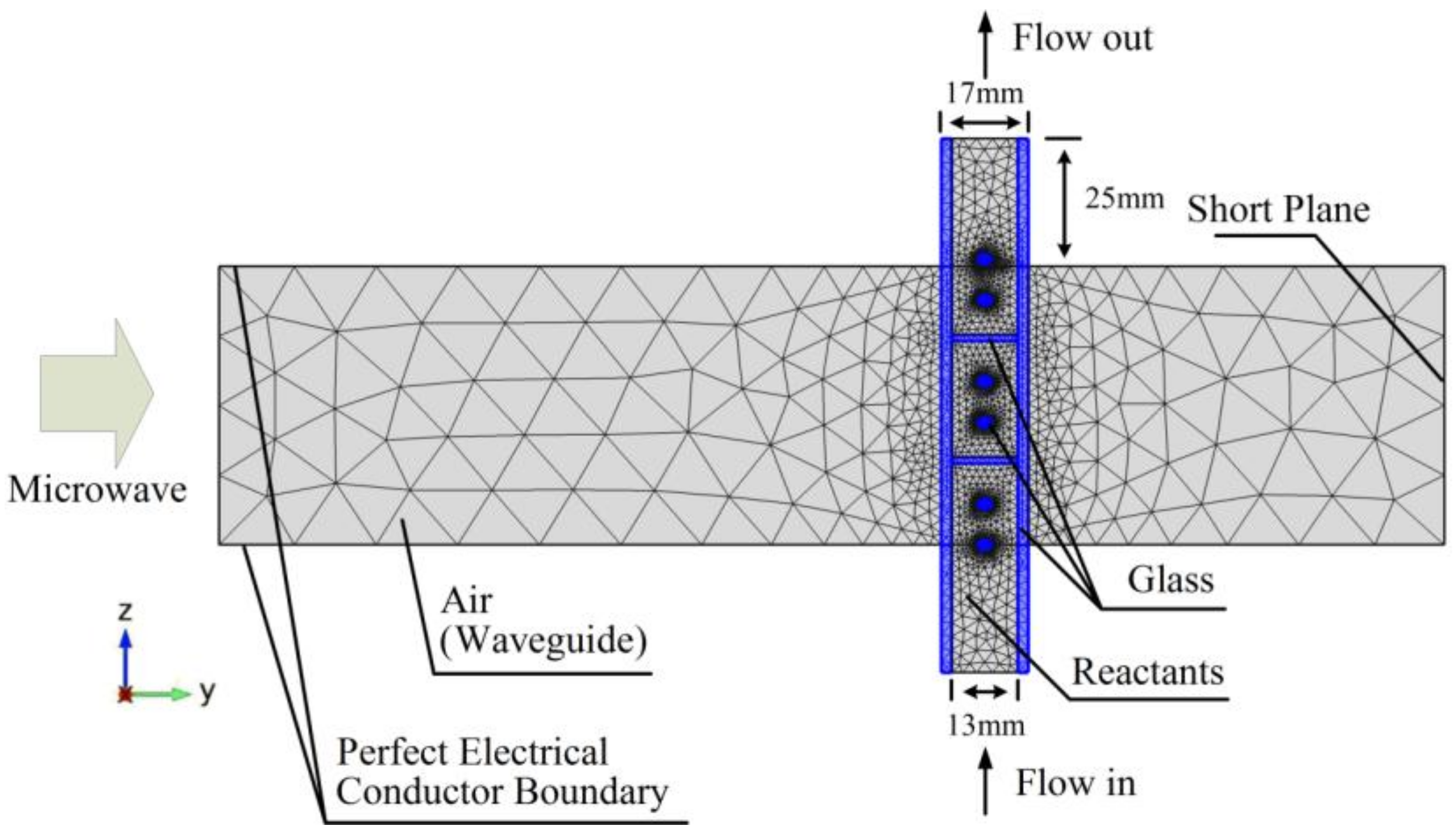
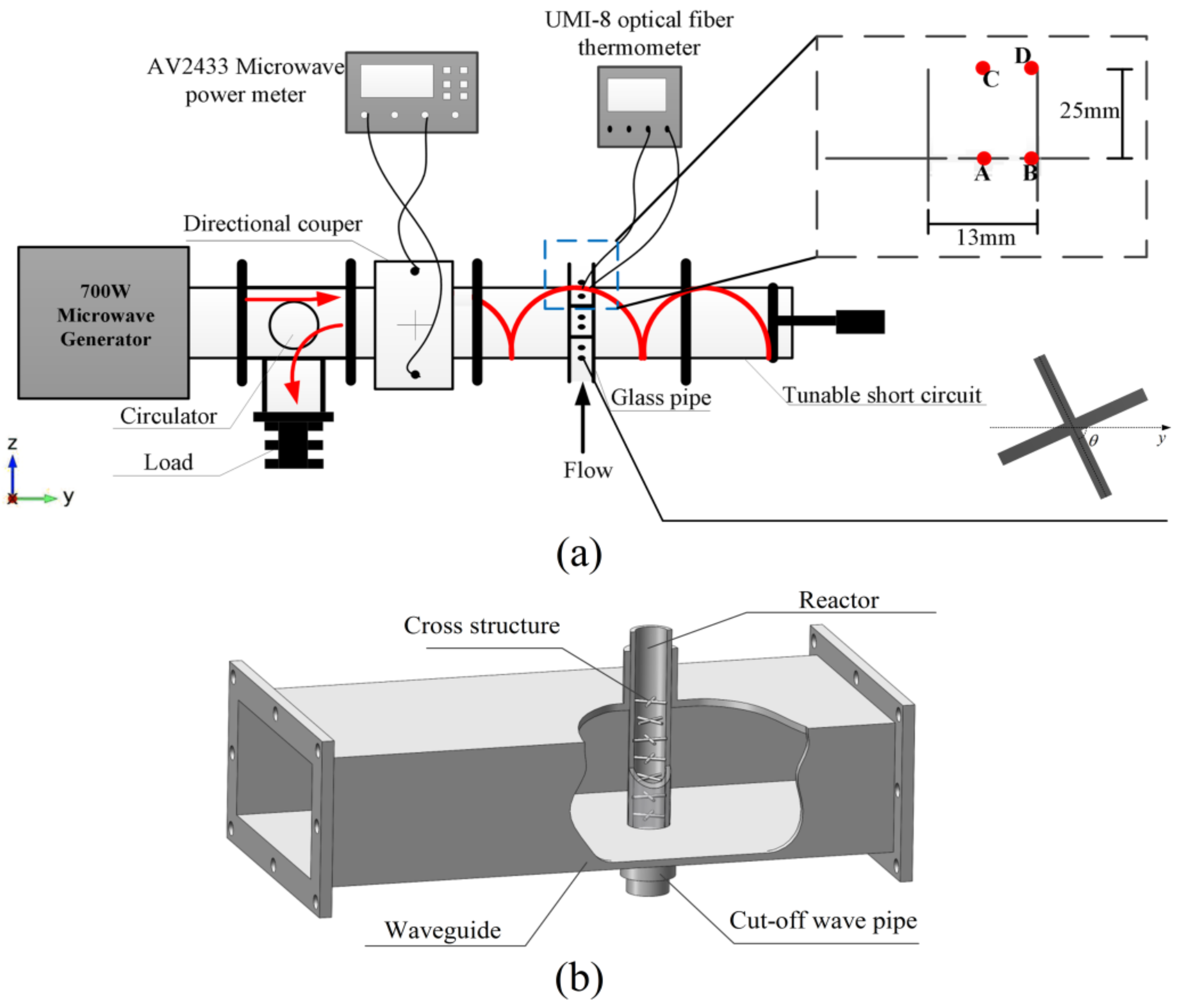
2.2. Experimental Setup
2.3. Calculation Model
2.4. Relative Permittivity
2.5. Thermal Model
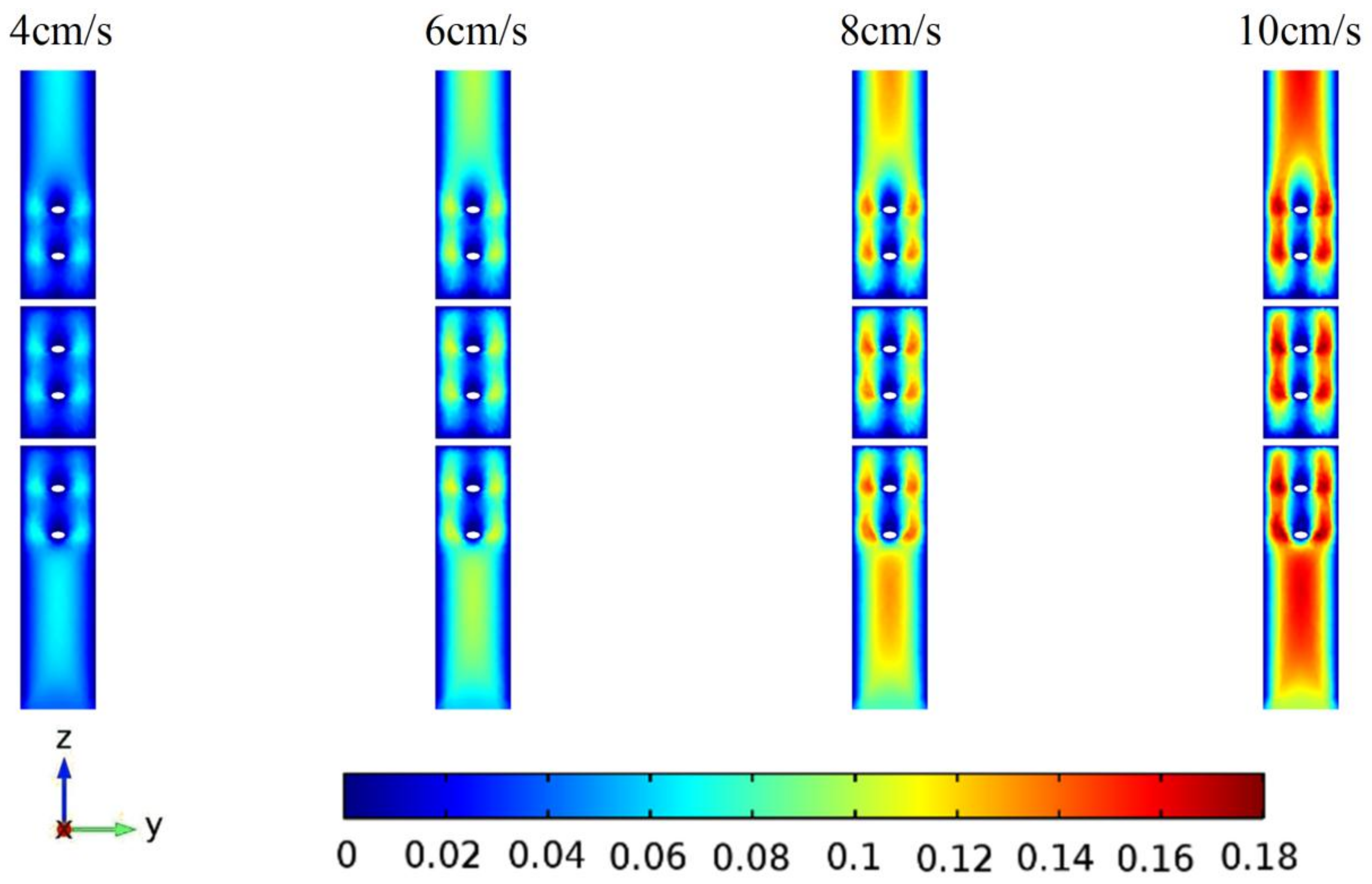
2.6. Flow Model
2.7. Chemical Reaction Kinetics
2.8. Mesh Size
2.9. Boundary Condition
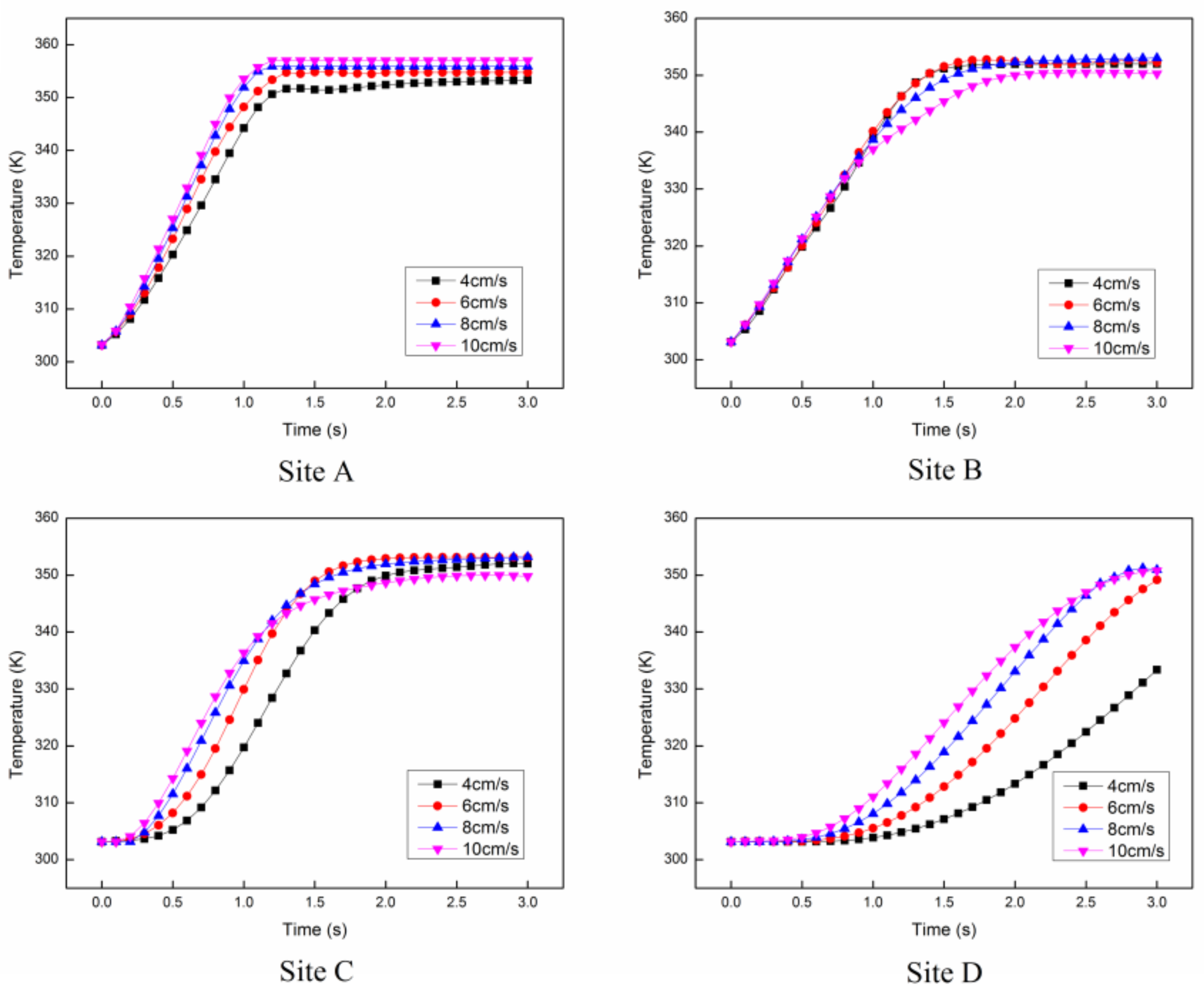
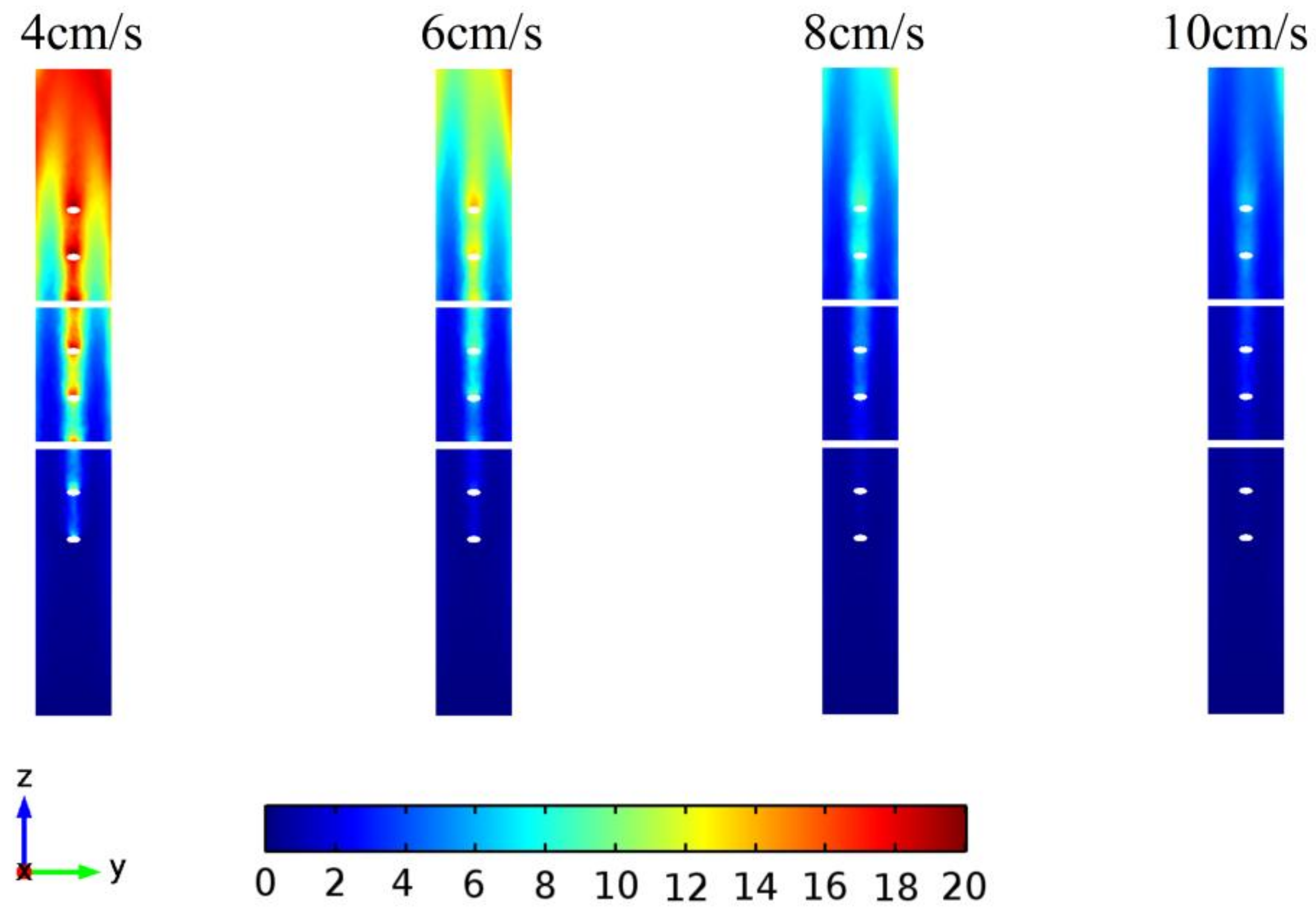
3. Results and Discussion
4. Conclusions
Acknowledgments
Author Contributions
Conflicts of Interest
References
- Weissermel, K.; Arpe, H. Industrial Organic Chemistry, 4th ed.; Wiley-VCH: Weinheim, Germany, 2003. [Google Scholar]
- Haslam, E. Recent developments in methods for the esterification and protection of the carboxyl group. Tetrahedron 1980, 36, 2409–2433. [Google Scholar] [CrossRef]
- Gnanadesikan, V.; Horiuchi, Y.; Ohshima, T.; Shibasaki, M. Direct catalytic asymmetric aldol-Tishchenko reaction. J. Am. Chem. Soc. 2004, 126, 7782–7783. [Google Scholar] [CrossRef] [PubMed]
- Gregory, R.; Smith, D.J.H.; Westlake, D.J. The production of ethyl acetate from ethylene and acetic acid using clay catalysts. Clay Miner. 1983, 18, 431–435. [Google Scholar] [CrossRef]
- Nielsen, M.; Junge, H.; Kammer, A.; Beller, M. Towards a Green Process for Bulk-Scale Synthesis of Ethyl Acetate: Efficient Acceptorless Dehydrogenation of Ethanol. Angew. Chem. Int. Ed. 2012, 51, 5711–5713. [Google Scholar] [CrossRef] [PubMed]
- Hong, T.; Tang, Z.; Zhu, H. Anomalous dielectric relaxation with linear reaction dynamics in space-dependent force fields. J. Chem. Phys. 2016, 145, 244105. [Google Scholar] [CrossRef] [PubMed]
- Li, K.; Hou, B.; Wang, L.; Cui, Y. Application of carbon nanocatalysts in upgrading heavy crude oil assisted with microwave heating. Nano Lett. 2014, 14, 3002–3008. [Google Scholar] [CrossRef] [PubMed]
- Meda, V.; Orsat, V.; Raghavan, V. Microwave heating and the dielectric properties of foods. In The Microwave Processing of Foods; Woodhead Publishing: Cambridge, UK, 2017; pp. 23–43. [Google Scholar]
- Pu, Y.Y.; Sun, D.W. Combined hot-air and microwave-vacuum drying for improving drying uniformity of mango slices based on hyperspectral imaging visualisation of moisture content distribution. Biosyst. Eng. 2017, 156, 108–119. [Google Scholar] [CrossRef]
- Ghasali, E.; Yazdani-Rad, R.; Asadian, K.; Ebadzadeh, T. Production of Al-SiC-TiC hybrid composites using pure and 1056 aluminum powders prepared through microwave and conventional heating methods. J. Alloys Compd. 2017, 690, 512–518. [Google Scholar] [CrossRef]
- Cheng, Y.; Zhang, Y.; Wan, T.; Yin, Z.; Wang, J. Mechanical properties and toughening mechanisms of graphene platelets reinforced Al2O3/TiC composite ceramic tool materials by microwave sintering. Mater. Sci. Eng. A 2017, 680, 190–196. [Google Scholar] [CrossRef]
- Fan, L.; Chen, P.; Zhang, Y.; Liu, S.; Liu, Y.; Wang, Y.; Dai, L.; Ruan, R. Fast microwave-assisted catalytic co-pyrolysis of lignin and low-density polyethylene with HZSM-5 and MgO for improved bio-oil yield and quality. Bioresour. Technol. 2017, 225, 199–205. [Google Scholar] [CrossRef] [PubMed]
- Loong, T.C.; Idris, A. One step transesterification of biodiesel production using simultaneous cooling and microwave heating. J. Clean. Prod. 2017, 146, 57–62. [Google Scholar] [CrossRef]
- Damm, M.; Glasnov, T.N.; Kappe, C.O. Translating high-temperature microwave chemistry to scalable continuous flow processes. Org. Process Res. Dev. 2009, 14, 215–224. [Google Scholar] [CrossRef]
- Horikoshi, S.; Osawa, A.; Abe, M.; Serpone, N. On the generation of hot-spots by microwave electric and magnetic fields and their impact on a microwave-assisted heterogeneous reaction in the presence of metallic Pd nanoparticles on an activated carbon support. J. Phys. Chem. C 2011, 115, 23030–23035. [Google Scholar] [CrossRef]
- Sebera, V.; Nasswettrová, A.; Nikl, K. Finite element analysis of mode stirrer impact on electric field uniformity in a microwave applicator. Dry. Technol. 2012, 30, 1388–1396. [Google Scholar] [CrossRef]
- Ye, J.; Hong, T.; Wu, Y.; Wu, L.; Liao, Y.; Zhu, H.; Yang, Y.; Huang, K. Model Stirrer Based on a Multi-Material Turntable for Microwave Processing Materials. Materials 2017, 10, 95. [Google Scholar] [CrossRef] [PubMed]
- Wu, X.; Thomas, J.R., Jr.; Davis, W.A. Control of thermal runaway in microwave resonant cavities. J. Appl. Phys. 2002, 92, 3374–3380. [Google Scholar] [CrossRef]
- Bows, J.R.; Patrick, M.L.; Janes, R.; Dibben, D.C. Microwave phase control heating. Int. J. Food Sci. Technol. 1999, 34, 295–304. [Google Scholar] [CrossRef]
- Patil, N.G.; Hermans, A.I.G.; Benaskar, F.; Meuldijk, J.; Hulshof, L.A.; Hessel, V.; Schouten, J.C.; Rebrov, E.V. Energy efficient and controlled flow processing under microwave heating by using a millireactor—Heat exchanger. AIChE J. 2012, 58, 3144–3155. [Google Scholar] [CrossRef]
- Patil, N.G.; Benaskar, F.; Benaskar, F.; Meuldijk, J.; Hulshof, L.A.; Hessel, V.; Schouten, J.C.; Esveld, E.D.C.; Rebrov, E.V. Microwave assisted flow synthesis: Coupling of electromagnetic and hydrodynamic phenomena. AIChE J. 2014, 60, 3824–3832. [Google Scholar] [CrossRef]
- Ge, W.F.; Hu, X.P.; Wu, J. Kinetics for esterification of acetic acid with ethanol catalyzed by sodium acid sulfate. Chem. React. Eng. Technol. 2010, 26, 264–268. (In Chinese) [Google Scholar]
- Liao, Y.; Lan, J.; Zhang, C.; Hong, T.; Yang, Y.; Huang, K.; Zhu, H. A Phase-Shifting Method for Improving the Heating Uniformity of Microwave Processing Materials. Materials 2016, 9, 309. [Google Scholar] [CrossRef] [PubMed]
- Huang, K.; Zhu, H.; Wu, L. Temperature cycle measurement for effective permittivity of biodiesel reaction. Bioresour. Technol. 2013, 131, 541–544. [Google Scholar] [CrossRef] [PubMed]
- Zhu, H.C.; Lan, J.Q.; Wu, L.; Gulati, T.; Chen, Q.; Hong, T.; Huang, K.M. Bivariate characterization and measurement for effective permittivity of esterification reactions at 2450 MHz for multiphysics simulation. Int. J. Appl. Electromagn. Mech. 2015, 47, 927–937. [Google Scholar] [CrossRef]
- Lide, D.R. CRC Handbook of Chemistry and Physics, 82nd ed.; Taylor & Francis group: Boca Raton, FL, USA, 2002. [Google Scholar]
- Li, X.; Chen, W.; Liu, G.; Lu, W.; Fu, J. Continuous-flow microfluidic blood cell sorting for unprocessed whole blood using surface-micromachined microfiltration membranes. Lab Chip 2014, 14, 2565–2575. [Google Scholar] [CrossRef] [PubMed]
- Hong, Y.; Lin, B.; Li, H.; Dai, H.; Zhu, C.; Yao, H. Three-dimensional simulation of microwave heating coal sample with varying parameters. Appl. Therm. Eng. 2016, 93, 1145–1154. [Google Scholar] [CrossRef]
- Zhu, J.; Kuznetsov, A.V.; Sandeep, K.P. Numerical simulation of forced convection in a duct subjected to microwave heating. Heat Mass Transf. 2007, 43, 255–264. [Google Scholar] [CrossRef]


| Parameter | Equation | |
|---|---|---|
| Thermal conductivity (W/m·K) | Ethanol | 0.2525 − 0.00028 × T |
| Acetic acid | 0.2128 − 0.000184 × T | |
| Ethyl acetate | 0.2513 − 0.00036 × T | |
| Water | 0.1896 + 0.0014 × T | |
| Density (kg/m3) | Ethanol | 789.3 |
| Acetic acid | 1049.2 | |
| Ethyl acetate | 900 | |
| Water | 1000 | |
| Specific heat capacity (J/kg·K) | Ethanol | 2440 |
| Acetic acid | 2055 | |
| Ethyl acetate | 1940 | |
| Water | 4200 | |
| Dynamic Viscosities (Pa·s) | Ethanol | 0.01809 − 0.00009572 × T + 0.0000001296 × T2 |
| Acetic acid | 0.009403 − 0.0000441 × T + 0.000000054 × T2 | |
| Ethyl acetate | 0.004058 − 0.00001983 × T + 0.0000000256 × T2 | |
| Water | 0.02478 − 0.0001409 × T + 0.0000002038 × T2 | |
| Initial Velocity (cm/s) | Site | Simulated Temperature (K) | Measured Temperature (K) | Error (%) |
|---|---|---|---|---|
| 4 | A | 353.1 | 350.90 | 0.623% |
| B | 351.9 | 350.55 | 0.384% | |
| 6 | A | 354.44 | 350.95 | 0.985% |
| B | 352.02 | 350.30 | 0.489% | |
| 8 | A | 355.59 | 349.85 | 1.614% |
| B | 353.05 | 349.80 | 0.921% | |
| 10 | A | 356.20 | 349.90 | 1.769% |
| B | 350.01 | 349.75 | 0.074% |
© 2018 by the authors. Licensee MDPI, Basel, Switzerland. This article is an open access article distributed under the terms and conditions of the Creative Commons Attribution (CC BY) license (http://creativecommons.org/licenses/by/4.0/).
Share and Cite
Wu, Y.; Hong, T.; Tang, Z.; Zhang, C. Dynamic Model for a Uniform Microwave-Assisted Continuous Flow Process of Ethyl Acetate Production. Entropy 2018, 20, 241. https://doi.org/10.3390/e20040241
Wu Y, Hong T, Tang Z, Zhang C. Dynamic Model for a Uniform Microwave-Assisted Continuous Flow Process of Ethyl Acetate Production. Entropy. 2018; 20(4):241. https://doi.org/10.3390/e20040241
Chicago/Turabian StyleWu, Yuanyuan, Tao Hong, Zhengming Tang, and Chun Zhang. 2018. "Dynamic Model for a Uniform Microwave-Assisted Continuous Flow Process of Ethyl Acetate Production" Entropy 20, no. 4: 241. https://doi.org/10.3390/e20040241
APA StyleWu, Y., Hong, T., Tang, Z., & Zhang, C. (2018). Dynamic Model for a Uniform Microwave-Assisted Continuous Flow Process of Ethyl Acetate Production. Entropy, 20(4), 241. https://doi.org/10.3390/e20040241