Amplitude- and Fluctuation-Based Dispersion Entropy


Abstract
1. Introduction
2. Methods
2.1. Dispersion Entropy (DispEn) with Different Mapping Techniques
- (1)
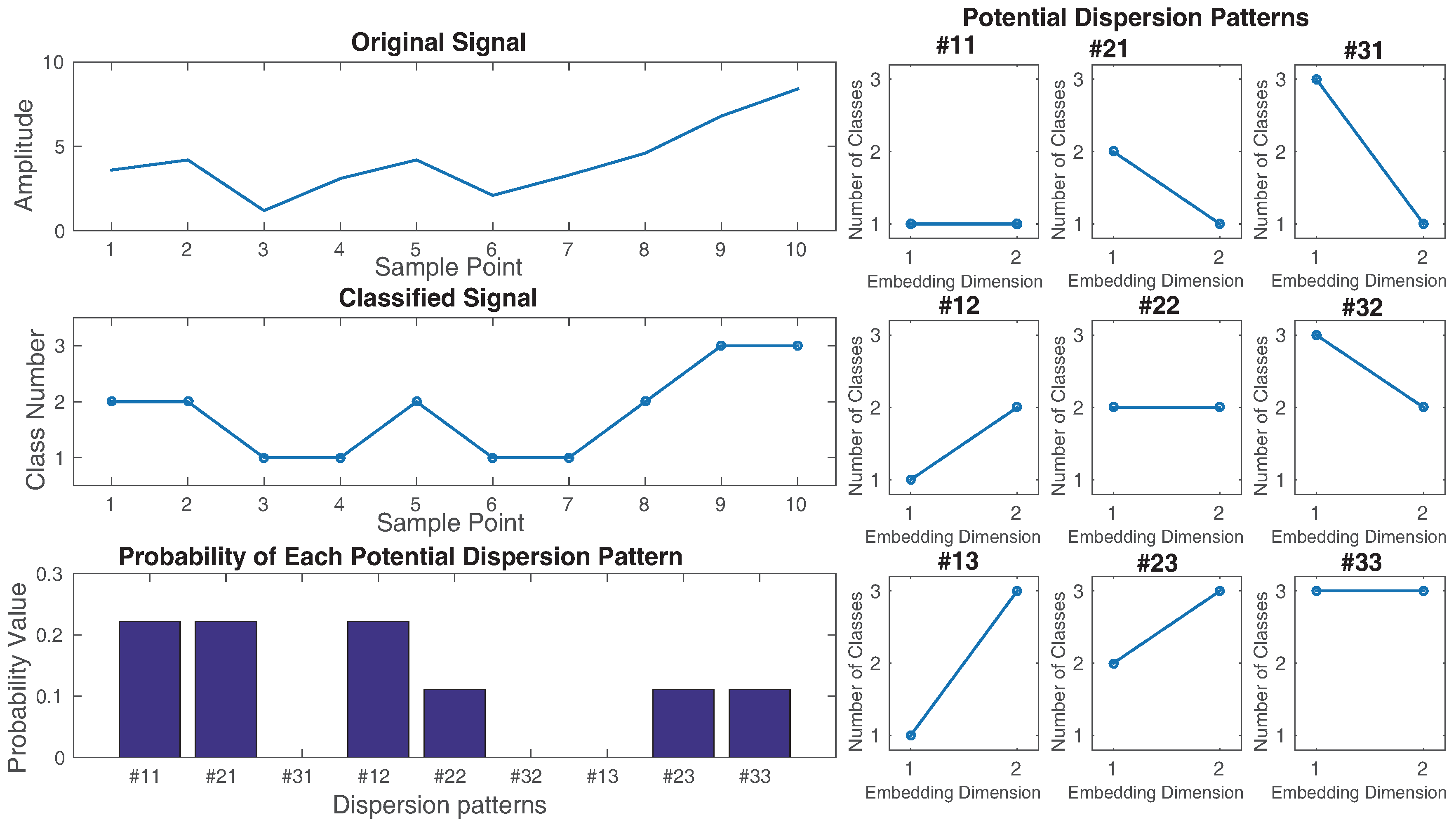
- First, are mapped to classes with integer indices from 1 to . The classified signal is . A number of linear and nonlinear mapping techniques, introduced in Section 2.3, can be used in this step.
- (2)
- Time series are made with embedding dimension m and time delay d according to , [9,10]. Each time series is mapped to a dispersion pattern , where , ,..., . The number of possible dispersion patterns assigned to each vector is equal to , since the signal has m elements and each can be one of the integers from 1 to c [9].
- (3)
- For each of potential dispersion patterns , relative frequency is obtained as follows:where # means cardinality. In fact, shows the number of dispersion patterns of that is assigned to , divided by the total number of embedded signals with embedding dimension m.
- (4)
- Finally, based on the Shannon’s definition of entropy, the DispEn value is calculated as follows:
2.2. Fluctuation-Based Dispersion Entropy (FDispEn)
2.3. Mapping Approaches Used in DispEn and FDispEn
3. Parameters of DispEn and FDispEn
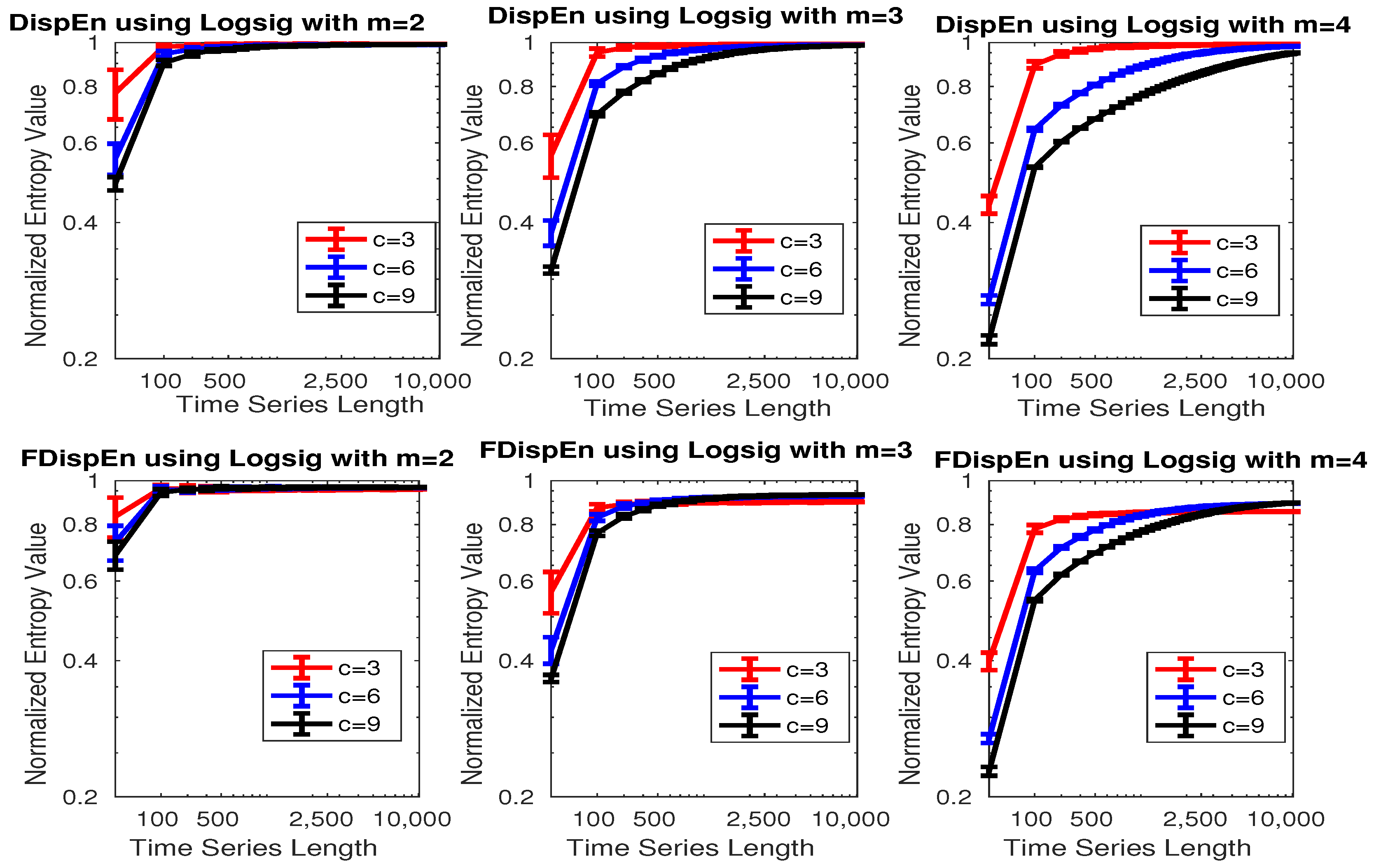
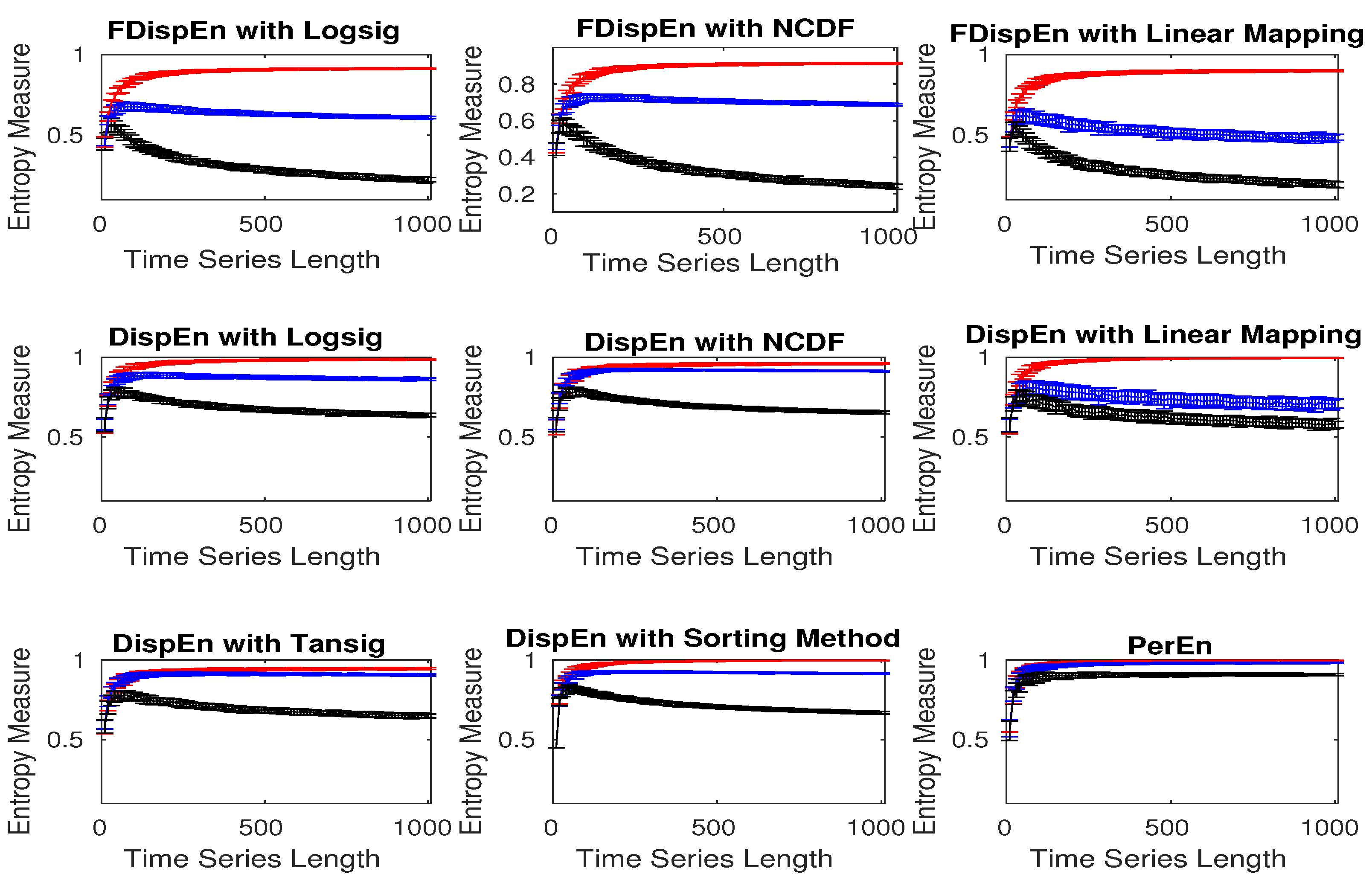
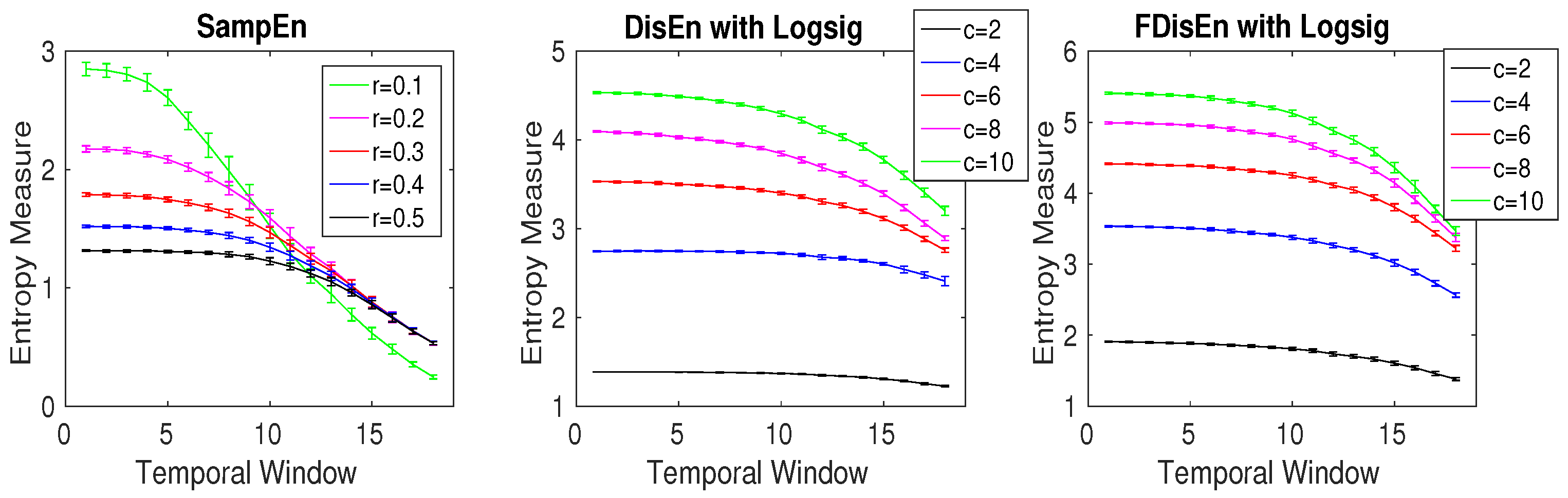
3.1. Effect of Number of Classes, Embedding Dimension, and Signal Length on DispEn and FDispEn
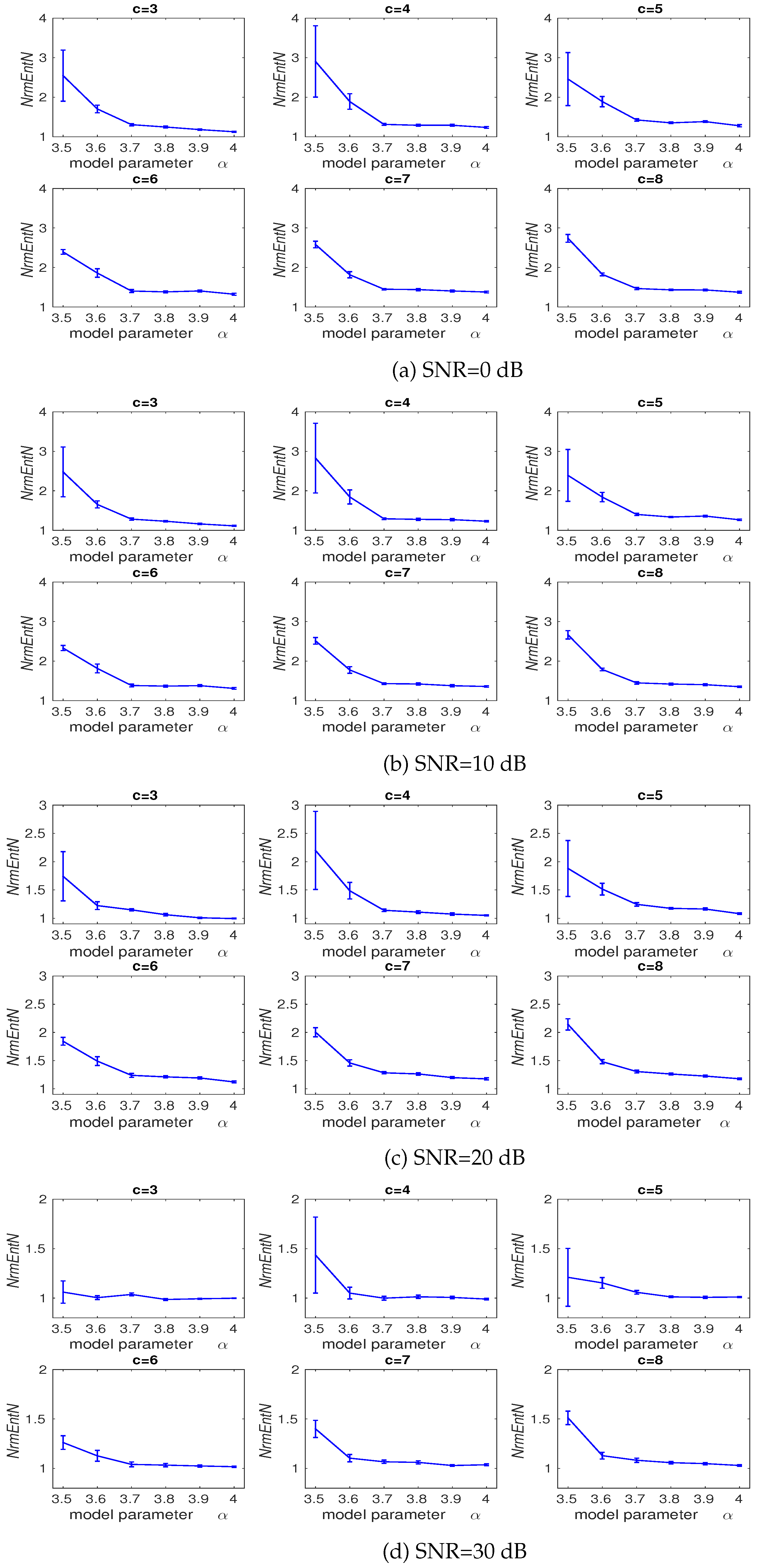
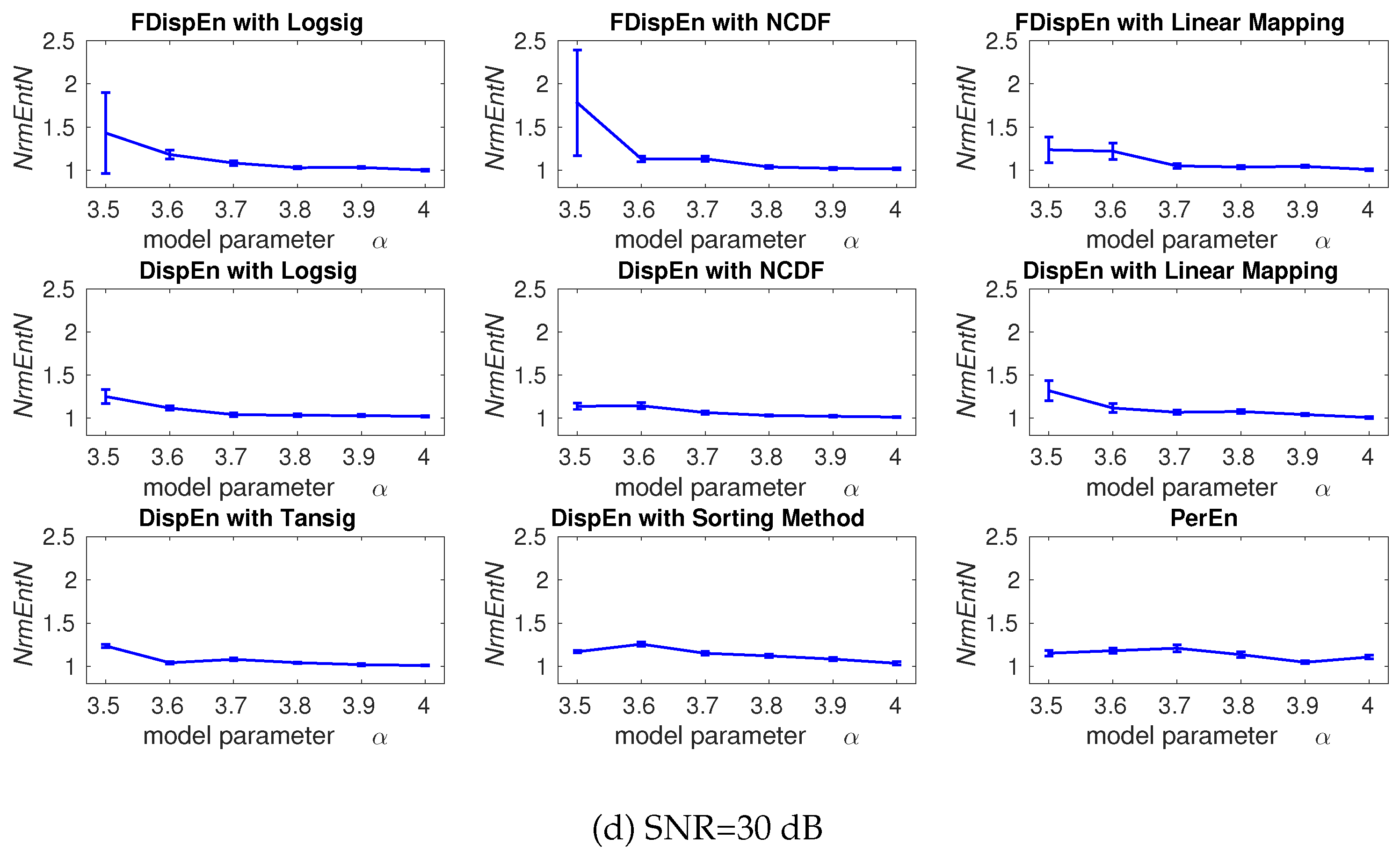
3.2. Effect of Number of Classes and Noise Power on DispEn and FDispEn
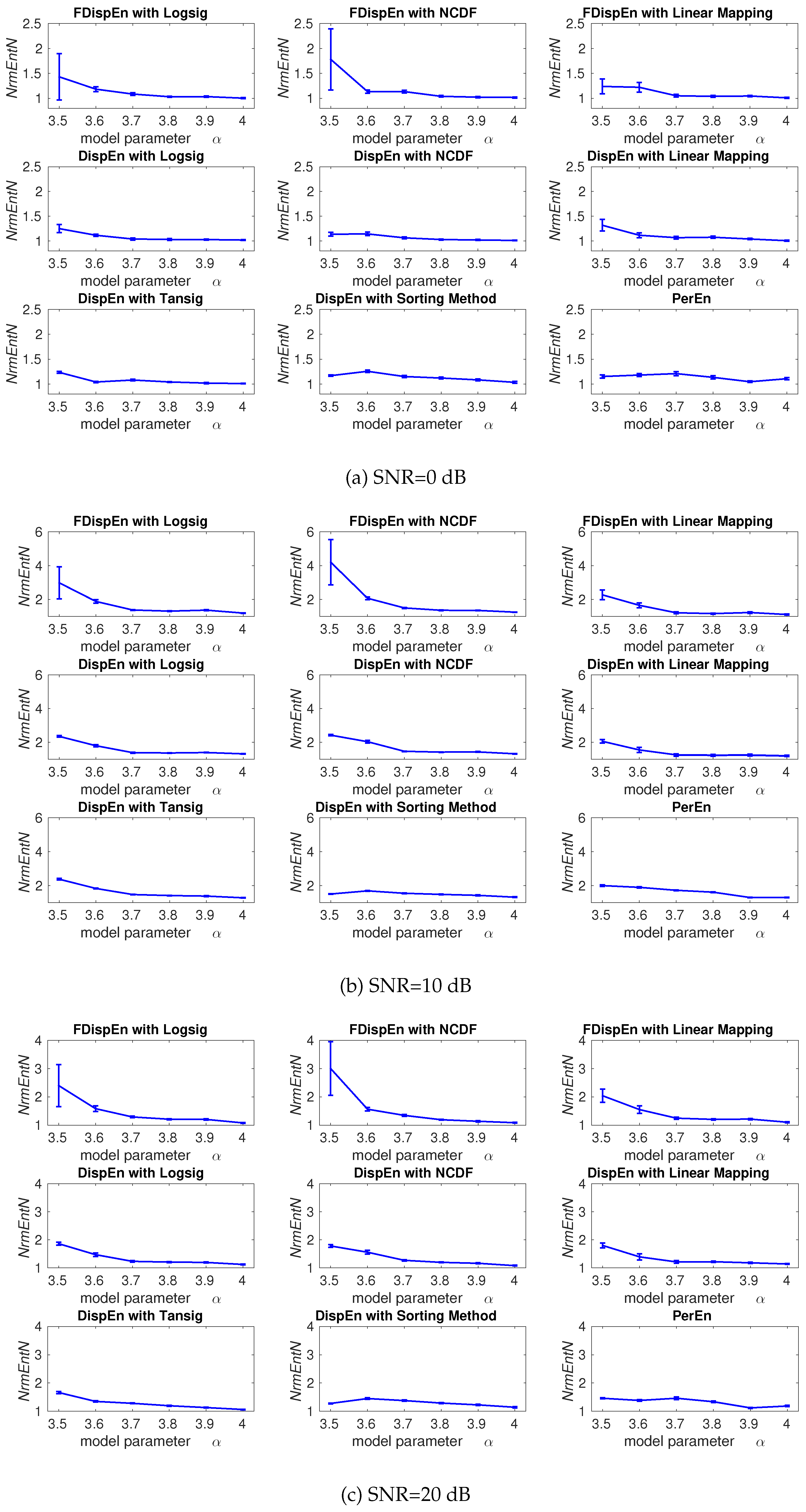
4. Evaluation of Mapping Approaches for DispEn and FDispEn
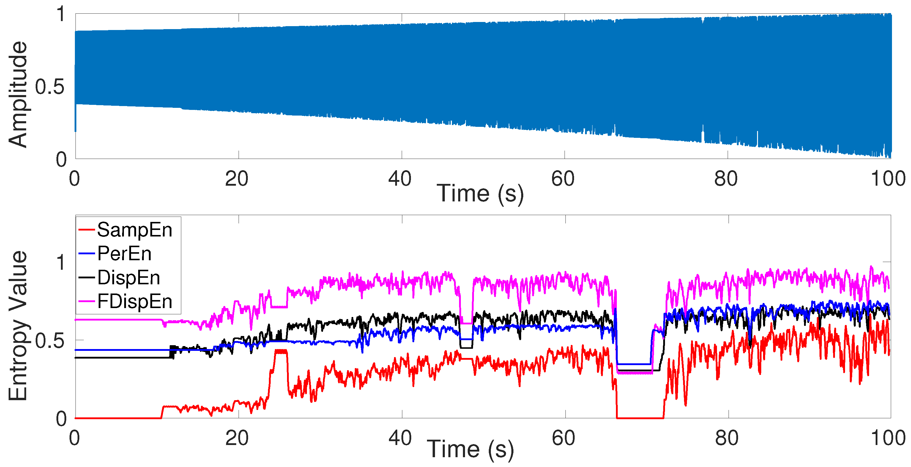
5. Univariate Entropy Methods vs. Changes from Periodicity to Non-Periodic Nonlinearity
6. Comparison Between SampEn, PerEn and Its Improvements, and Newly Developed DispEn and FDispEn
6.1. SampEn vs. DispEn and FDispEn
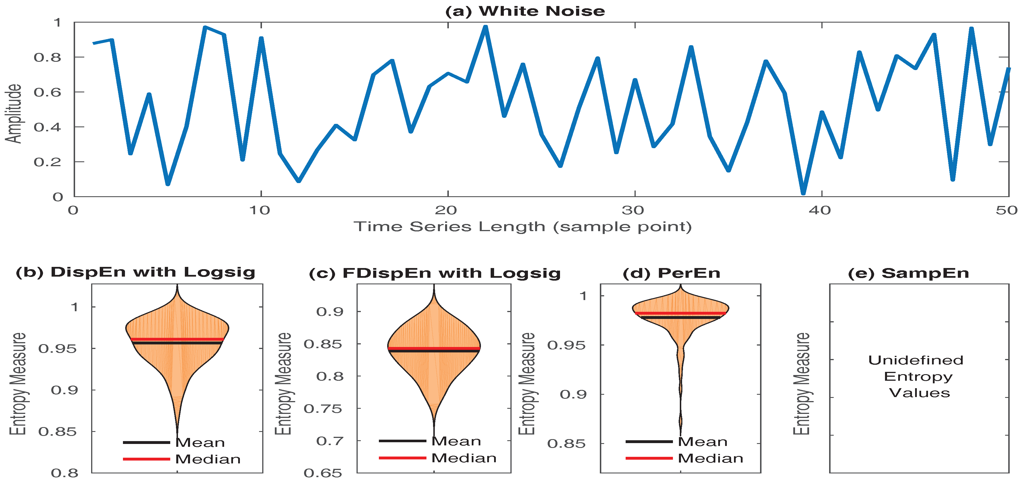
- SampEn values for short signals are either undefined or unreliable, as in its algorithm, the number of matches whose differences are smaller than a defined threshold is counted. When the time series length is too small, this number may be 0, leading to undefined values [16,53]. However, the results obtained by DispEn, FDispEn, and PerEn are always defined. To illustrate this issue, we created 40 realizations of white noise with length 50 sample points. The mean and median of DispEn, FDispEn, PerEn, and SampEn values for the 40 realizations are shown in Figure 8. The results show that SampEn, unlike DispEn, FDispEn, and PerEn, yield undefined values. Note that we set for SampEn, DispEn, and FDispEn, and for PerEn, as advised before.
6.2. PerEn and Its Improvements vs. DispEn and FDispEn
- PerEn considers only the order of amplitude values, and, thus, some information regarding the amplitude values themselves may be ignored [18]. For example, the embedded vectors and have similar permutations, leading to the same motif (0,2,1) () because the extent of the differences between sequential samples is not considered in the original definition of PerEn. To alleviate this deficiency, modified PerEn (MPerEn) based on mapping equal values into the same symbol was developed [17]. However, the second and third shortcomings were not addressed by MPerEn. Amplitude-aware PerEn (AAPerEn) deals with the problem with adding a variable contribution, depending on amplitude, instead of a constant number to each level in the histogram representing the probability of each motif [7]. It was also addressed by the use of modified ordinal patterns [56]. Mapping data to a number of classes based on their amplitude values makes DispEn and FDispEn deal with this issue as well.
- When there are equal values in the embedded vector, Bandt and Pompe [10] proposed ranking the possible equalities based on their order of emergence or solving this condition by adding noise. Considering the first alternative, for instance, the permutation pattern for both the embedded vectors and are (0,1,2) (). As another example, assume and . The PerEn with of is exactly the same as , both equalling 0 although, unlike , is strictly ascending. Adding noise may not lead to a precise answer because, for example, the embedded vector has two possible permutation patterns as (0,1,2) and (0,2,1) and there are not any differences between them. It should be noted that this issue is particularly relevant for digitized signals with large quantization steps. Fadlallah et al. have recently proposed weighted PerEn (WPerEn) to weight the motif counts by statistics derived from the time series patterns [8]. However, WPerEn does not take into account the first and third alleviations of PerEn. It was addressed in AAPerEn [7] as well. Assigning close amplitude values to an equal class, FDispEn and DispEn deal with this deficiency.
- PerEn is sensitive to noise (even when the SNR of a signal is high), since a small change in amplitude value may vary the order relations among amplitudes. For instance, noise on may alter the motif from (0,1,2) to (0,2,1). This problem is present for WPerEn, MPerEn, AAPerEn, and the approach developed in [56]. However, DispEn and FDispEn address the problem with mapping data into a few classes and, thus, a small change in amplitude will probably not alter the (index of) class.
7. Computation Cost of DispEn, FDispEn, and PerEn
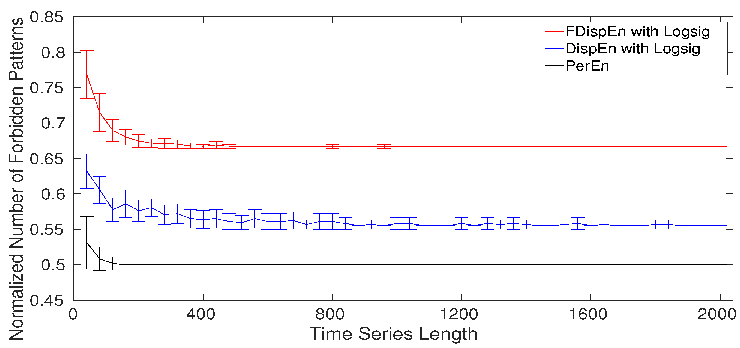
8. Forbidden Amplitude- and Fluctuation-Based Dispersion Patterns
- Step 1: Null hypothesis. We have all the dispersion patterns, while the permutation pattern does not exist for the signal x.
- Step 2: Rejection of null hypothesis. As the permutation pattern does not exist, we do not have any dispersion patterns sorted as . This is in contradiction with the fact that we have all the dispersion patterns for x. Hence, the null hypothesis is rejected.
- Step 3: Conclusion. When we have all the dispersion patterns, all the permutation patterns are present too. It confirms the fact that a forbidden permutation pattern leads to several forbidden dispersion patterns. Thus, if a signal is deterministic, and so does not have several permutation patterns, there are a number of forbidden dispersion patterns. Consequently, lack of dispersion patterns, like permutation patterns [57,58], reflects the deterministic behavior of a signal.
9. Applications of DispEn and FDispEn to Biomedical Time Series
9.1. Blood Pressure in Rats
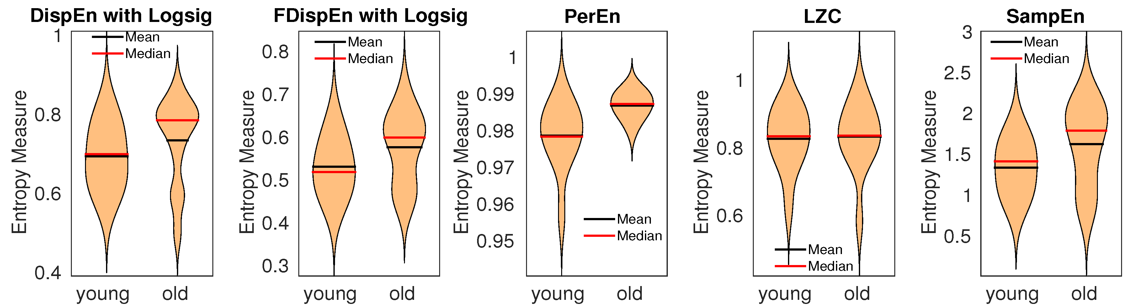
9.2. Gait Maturation Database
10. Conclusions
Author Contributions
Conflicts of Interest
References
- Bishop, C.M. Pattern Recognition and Machine Learning; Springer: New York, NY, USA, 2006. [Google Scholar]
- Biggs, N.L. The roots of combinatorics. Hist. Math. 1979, 6, 109–136. [Google Scholar] [CrossRef]
- Donald, E.K. The art of computer programming. Sort. Search. 1999, 3, 426–458. [Google Scholar]
- Keller, K.; Unakafov, A.M.; Unakafova, V.A. Ordinal patterns, entropy, and EEG. Entropy 2014, 16, 6212–6239. [Google Scholar] [CrossRef]
- Amigó, J. Permutation Complexity in Dynamical Systems: Ordinal Patterns, Permutation Entropy and All That; Springer: Heidelberg, Germany; London, UK, 2010. [Google Scholar]
- Steingrımsson, E. Generalized permutation patterns—A short survey. Permut. Patterns 2010, 376, 137–152. [Google Scholar]
- Azami, H.; Escudero, J. Amplitude-aware permutation entropy: Illustration in spike detection and signal segmentation. Comput. Methods Programs Biomed. 2016, 128, 40–51. [Google Scholar] [CrossRef] [PubMed]
- Fadlallah, B.; Chen, B.; Keil, A.; Príncipe, J. Weighted-permutation entropy: A complexity measure for time series incorporating amplitude information. Phys. Rev. E 2013, 87, 022911. [Google Scholar] [CrossRef] [PubMed]
- Rostaghi, M.; Azami, H. Dispersion entropy: A measure for time series analysis. IEEE Signal Process. Lett. 2016, 23, 610–614. [Google Scholar] [CrossRef]
- Bandt, C.; Pompe, B. Permutation entropy: A natural complexity measure for time series. Phys. Rev. Lett. 2002, 88, 174102. [Google Scholar] [CrossRef] [PubMed]
- Shannon, C.E. A mathematical theory of communication. ACM SIGMOBILE Mob. Comput. Commun. Rev. 2001, 5, 3–55. [Google Scholar] [CrossRef]
- Faes, L.; Porta, A.; Nollo, G. Information decomposition in bivariate systems: Theory and application to cardiorespiratory dynamics. Entropy 2015, 17, 277–303. [Google Scholar] [CrossRef]
- Costa, M.; Goldberger, A.L.; Peng, C.K. Multiscale entropy analysis of biological signals. Phys. Rev. E 2005, 71, 021906. [Google Scholar] [CrossRef] [PubMed]
- Richman, J.S.; Moorman, J.R. Physiological time-series analysis using approximate entropy and sample entropy. Am. J. Physiol.-Heart Circ. Physiol. 2000, 278, H2039–H2049. [Google Scholar] [CrossRef] [PubMed]
- Wu, S.D.; Wu, C.W.; Humeau-Heurtier, A. Refined scale-dependent permutation entropy to analyze systems complexity. Phys. A Stat. Mech. Appl. 2016, 450, 454–461. [Google Scholar] [CrossRef]
- Azami, H.; Fernández, A.; Escudero, J. Refined multiscale fuzzy entropy based on standard deviation for biomedical signal analysis. Med. Biol. Eng. Comput. 2017, 55, 2037–2052. [Google Scholar] [CrossRef] [PubMed]
- Bian, C.; Qin, C.; Ma, Q.D.; Shen, Q. Modified permutation-entropy analysis of heartbeat dynamics. Phys. Rev. E 2012, 85, 021906. [Google Scholar] [CrossRef] [PubMed]
- Zanin, M.; Zunino, L.; Rosso, O.A.; Papo, D. Permutation entropy and its main biomedical and econophysics applications: A review. Entropy 2012, 14, 1553–1577. [Google Scholar] [CrossRef]
- Kurths, J.; Voss, A.; Saparin, P.; Witt, A.; Kleiner, H.; Wessel, N. Quantitative analysis of heart rate variability. Chaos Interdiscip. J. Nonlinear Sci. 1995, 5, 88–94. [Google Scholar] [CrossRef] [PubMed]
- Hao, B.L. Symbolic dynamics and characterization of complexity. Phys. D Nonlinear Phenom. 1991, 51, 161–176. [Google Scholar] [CrossRef]
- Voss, A.; Kurths, J.; Kleiner, H.; Witt, A.; Wessel, N. Improved analysis of heart rate variability by methods of nonlinear dynamics. J. Electrocardiol. 1995, 28, 81–88. [Google Scholar] [CrossRef]
- Azami, H.; Rostaghi, M.; Fernández, A.; Escudero, J. Dispersion entropy for the analysis of resting-state MEG regularity in Alzheimer’s disease. In Proceedings of the 2016 IEEE 38th Annual International Conference of the Engineering in Medicine and Biology Society (EMBC), Orlando, FL, USA, 16–20 August 2016; pp. 6417–6420. [Google Scholar]
- Mitiche, I.; Morison, G.; Nesbitt, A.; Boreham, P.; Stewart, B.G. Classification of partial discharge EMI conditions using permutation entropy-based features. In Proceedings of the 2017 25th European Signal Processing Conference (EUSIPCO), Kos, Greece, 28 August–2 September 2017; pp. 1375–1379. [Google Scholar]
- Baldini, G.; Giuliani, R.; Steri, G.; Neisse, R. Physical layer authentication of Internet of Things wireless devices through permutation and dispersion entropy. In Proceedings of the 2017 IEEE Global Internet of Things Summit (GIoTS), Geneva, Switzerland, 6–9 June 2017; pp. 1–6. [Google Scholar]
- Hu, K.; Ivanov, P.C.; Chen, Z.; Carpena, P.; Stanley, H.E. Effect of trends on detrended fluctuation analysis. Phys. Rev. E 2001, 64, 011114. [Google Scholar] [CrossRef] [PubMed]
- Wu, Z.; Huang, N.E.; Long, S.R.; Peng, C.K. On the trend, detrending, and variability of nonlinear and nonstationary time series. Proc. Natl. Acad. Sci. USA 2007, 104, 14889–14894. [Google Scholar] [CrossRef] [PubMed]
- Peng, C.K.; Havlin, S.; Stanley, H.E.; Goldberger, A.L. Quantification of scaling exponents and crossover phenomena in nonstationary heartbeat time series. Chaos Interdiscip. J. Nonlinear Sci. 1995, 5, 82–87. [Google Scholar] [CrossRef] [PubMed]
- Tufféry, S. Data Mining and Statistics for Decision Making; Wiley: Chichester, UK, 2011. [Google Scholar]
- Baranwal, G.; Vidyarthi, D.P. Admission control in cloud computing using game theory. J. Supercomput. 2016, 72, 317–346. [Google Scholar] [CrossRef]
- Gibbs, M.N.; MacKay, D.J. Variational Gaussian process classifiers. IEEE Trans. Neural Netw. 2000, 11, 1458–1464. [Google Scholar] [PubMed]
- Duch, W. Uncertainty of data, fuzzy membership functions, and multilayer perceptrons. IEEE Trans. Neural Netw. 2005, 16, 10–23. [Google Scholar] [CrossRef] [PubMed]
- Pincus, S.M.; Goldberger, A.L. Physiological time-series analysis: What does regularity quantify? Am. J. Physiol.-Heart Circ. Physiol. 1994, 266, H1643–H1656. [Google Scholar] [CrossRef] [PubMed]
- Goldberger, A.L.; Peng, C.K.; Lipsitz, L.A. What is physiologic complexity and how does it change with aging and disease? Neurobiol. Aging 2002, 23, 23–26. [Google Scholar] [CrossRef]
- Goldberger, A.L.; Amaral, L.A.N.; Glass, L.; Hausdorff, J.M.; Ivanov, P.C.; Mark, R.G.; Mietus, J.E.; Moody, G.B.; Peng, C.-K.; Stanley, H.E. PhysioBank, PhysioToolkit, and PhysioNet—Components of a New Research Resource for Complex Physiologic Signals. Circulation 2000, 101, e215–e220. [Google Scholar] [CrossRef] [PubMed]
- Pincus, S.M. Approximate entropy as a measure of system complexity. Proc. Natl. Acad. Sci. USA 1991, 88, 2297–2301. [Google Scholar] [CrossRef] [PubMed]
- Li, P.; Liu, C.; Li, K.; Zheng, D.; Liu, C.; Hou, Y. Assessing the complexity of short-term heartbeat interval series by distribution entropy. Med. Biol. Eng. Comput. 2015, 53, 77–87. [Google Scholar] [CrossRef] [PubMed]
- Aboy, M.; Hornero, R.; Abásolo, D.; Álvarez, D. Interpretation of the Lempel–Ziv complexity measure in the context of biomedical signal analysis. IEEE Trans. Biomed. Eng. 2006, 53, 2282–2288. [Google Scholar] [CrossRef] [PubMed]
- Ferrario, M.; Signorini, M.G.; Magenes, G.; Cerutti, S. Comparison of entropy-based regularity estimators: Application to the fetal heart rate signal for the identification of fetal distress. IEEE Trans. Biomed. Eng. 2006, 53, 119–125. [Google Scholar] [CrossRef] [PubMed]
- Baker, G.L.; Gollub, J.P. Chaotic Dynamics: An Introduction; Cambridge University Press: Cambridge, UK, 1996. [Google Scholar]
- Lam, J. Preserving Useful info while Reducing Noise of Physiological Signals by Using Wavelet Analysis. Master’s Thesis, Electrical Engineering University of North Florida, Jacksonville, FL, USA, 2011. [Google Scholar]
- Houdré, C.; Mason, D.M.; Reynaud-Bouret, P.; Rosinski, J. High Dimensional Probability VII; Springer: Basel, Switzerland, 2016; pp. 1–6. [Google Scholar]
- Escudero, J.; Hornero, R.; Abásolo, D. Interpretation of the auto-mutual information rate of decrease in the context of biomedical signal analysis. Application to electroencephalogram recordings. Physiol. Meas. 2009, 30, 187. [Google Scholar] [CrossRef] [PubMed]
- Azami, H.; Rostaghi, M.; Abasolo, D.; Escudero, J. Refined Composite Multiscale Dispersion Entropy and its Application to Biomedical Signals. IEEE Trans. Biomed. Eng. 2017, 64, 2872–2879. [Google Scholar] [CrossRef] [PubMed]
- Cohen, L. The history of noise (on the 100th anniversary of its birth). IEEE Signal Process. Mag. 2005, 22, 20–45. [Google Scholar] [CrossRef]
- Sejdić, E.; Lipsitz, L.A. Necessity of noise in physiology and medicine. Comput. Methods Programs Biomed. 2013, 111, 459–470. [Google Scholar] [CrossRef] [PubMed]
- Keshner, M.S. 1/f noise. Proc. IEEE 1982, 70, 212–218. [Google Scholar] [CrossRef]
- Azami, H.; Smith, K.; Fernandez, A.; Escudero, J. Evaluation of resting-state magnetoencephalogram complexity in Alzheimer’s disease with multivariate multiscale permutation and sample entropies. In Proceedings of the 2015 37th Annual International Conference of the IEEE Engineering in Medicine and Biology Society (EMBC), Milan, Italy, 25–29 August 2015; pp. 7422–7425. [Google Scholar]
- Kowalski, A.; Martín, M.; Plastino, A.; Rosso, O. Bandt–Pompe approach to the classical-quantum transition. Phys. D Nonlinear Phenom. 2007, 233, 21–31. [Google Scholar] [CrossRef]
- Mitov, I. A method for assessment and processing of biomedical signals containing trend and periodic components. Med. Eng. Phys. 1998, 20, 660–668. [Google Scholar] [CrossRef]
- Bahr, D.E.; Reuss, J.L. Method and Apparatus for Processing a Physiological Signal. U.S. Patent 6,339,715, 15 January 2002. [Google Scholar]
- Hornero, R.; Abásolo, D.; Escudero, J.; Gómez, C. Nonlinear analysis of electroencephalogram and magnetoencephalogram recordings in patients with Alzheimer’s disease. Philos. Trans. R. Soc. Lond. A Math. Phys. Eng. Sci. 2009, 367, 317–336. [Google Scholar] [CrossRef] [PubMed]
- Stam, C.J. Nonlinear dynamical analysis of EEG and MEG: Review of an emerging field. Clin. Neurophysiol. 2005, 116, 2266–2301. [Google Scholar] [CrossRef] [PubMed]
- Wu, S.D.; Wu, C.W.; Lin, S.G.; Lee, K.Y.; Peng, C.K. Analysis of complex time series using refined composite multiscale entropy. Phys. Lett. A 2014, 378, 1369–1374. [Google Scholar] [CrossRef]
- Jiang, Y.; Mao, D.; Xu, Y. A fast algorithm for computing sample entropy. Adv. Adapt. Data Anal. 2011, 3, 167–186. [Google Scholar] [CrossRef]
- Humeau-Heurtier, A.; Wu, C.W.; Wu, S.D. Refined composite multiscale permutation entropy to overcome multiscale permutation entropy length dependence. IEEE Signal Process. Lett. 2015, 22, 2364–2367. [Google Scholar] [CrossRef]
- Unakafova, V.A.; Keller, K. Efficiently measuring complexity on the basis of real-world data. Entropy 2013, 15, 4392–4415. [Google Scholar] [CrossRef]
- Carpi, L.C.; Saco, P.M.; Rosso, O. Missing ordinal patterns in correlated noises. Phys. A Stat. Mech. Appl. 2010, 389, 2020–2029. [Google Scholar] [CrossRef]
- Amigó, J.M.; Zambrano, S.; Sanjuán, M.A. True and false forbidden patterns in deterministic and random dynamics. EPL (Europhys. Lett.) 2007, 79, 50001. [Google Scholar] [CrossRef]
- Sleimen-Malkoun, R.; Perdikis, D.; Müller, V.; Blanc, J.L.; Huys, R.; Temprado, J.J.; Jirsa, V.K. Brain dynamics of aging: Multiscale variability of EEG signals at rest and during an auditory oddball task. Eneuro 2015, 2, e0067-14.2015. [Google Scholar] [CrossRef] [PubMed]
- Andrzejak, R.G.; Lehnertz, K.; Mormann, F.; Rieke, C.; David, P.; Elger, C.E. Indications of nonlinear deterministic and finite-dimensional structures in time series of brain electrical activity: Dependence on recording region and brain state. Phys. Rev. E 2001, 64, 061907. [Google Scholar] [CrossRef] [PubMed]
- Hoyer, D.; Leder, U.; Hoyer, H.; Pompe, B.; Sommer, M.; Zwiener, U. Mutual information and phase dependencies: Measures of reduced nonlinear cardiorespiratory interactions after myocardial infarction. Med. Eng. Phys. 2002, 24, 33–43. [Google Scholar] [CrossRef]
- Palacios, M.; Friedrich, H.; Götze, C.; Vallverdú, M.; de Luna, A.B.; Caminal, P.; Hoyer, D. Changes of autonomic information flow due to idiopathic dilated cardiomyopathy. Physiol. Meas. 2007, 28, 677. [Google Scholar] [CrossRef] [PubMed]
- Fares, S.A.; Habib, J.R.; Engoren, M.C.; Badr, K.F.; Habib, R.H. Effect of salt intake on beat-to-beat blood pressure nonlinear dynamics and entropy in salt-sensitive versus salt-protected rats. Physiol. Rep. 2016, 4, e12823. [Google Scholar] [CrossRef] [PubMed]
- Rosenthal, R. Parametric measures of effect size. In The Handbook of Research Synthesis; Cooper, H., Hedges, L.V., Eds.; Russell Sage Foundation: New York, NY, USA, 1994; pp. 231–244. [Google Scholar]
- Hausdorff, J.; Zemany, L.; Peng, C.K.; Goldberger, A. Maturation of gait dynamics: Stride-to-stride variability and its temporal organization in children. J. Appl. Physiol. 1999, 86, 1040–1047. [Google Scholar] [CrossRef] [PubMed]
- Hong, S.L.; James, E.G.; Newell, K.M. Age-related complexity and coupling of children’s sitting posture. Dev. Psychobiol. 2008, 50, 502–510. [Google Scholar] [CrossRef] [PubMed]
- Bisi, M.; Stagni, R. Complexity of human gait pattern at different ages assessed using multiscale entropy: From development to decline. Gait Posture 2016, 47, 37–42. [Google Scholar] [CrossRef] [PubMed]


| Method | |||||
| DispEn | 0.0021 | 0.0034 | 0.0045 | 0.0041 | 0.0048 |
| FDispEn | 0.0078 | 0.0064 | 0.0040 | 0.0043 | 0.0049 |
| SD | SD | SD | SD | SD | |
| SampEn | 0.0604 | 0.0342 | 0.0224 | 0.0174 | 0.0150 |
| Characteristics | DispEn | FDispEn | AAPerEn | PerEn | SampEn |
|---|---|---|---|---|---|
| Short signals | reliable | reliable | reliable | reliable | undefined |
| Sensitivity to noise | no | no | yes | yes | no |
| Type of entropy | ShEn | ShEn | ShEn | ShEn | ConEn |
| Computational cost | O(N) | O(N) | O(N) | O(N) | O() |
| Number of Samples | 300 | 1000 | 3000 | 10,000 | 30,000 | 100,000 |
|---|---|---|---|---|---|---|
| DispEn () | 0.0022 s | 0.0022 s | 0.0025 s | 0.0057 s | 0.0080 s | 0.0225 s |
| DispEn () | 0.0028 s | 0.0035 s | 0.0076 s | 0.0115 s | 0.0284 s | 0.0888 s |
| DispEn () | 0.0084 s | 0.0094 s | 0.0205 s | 0.0505 s | 0.1422 s | 0.4752 s |
| FDispEn () | 0.0022 s | 0.0025 s | 0.0028 s | 0.0034 s | 0.0062 s | 0.0175 s |
| FDispEn () | 0.0025 s | 0.0031 s | 0.0038 s | 0.0062 s | 0.0150 s | 0.0490 s |
| FDispEn () | 0.0054 s | 0.0064 s | 0.0120 s | 0.0284 s | 0.0699 s | 0.2535 s |
| SampEn () | 0.0023 s | 0.0208 s | 0.1841 s | 1.8478 s | 16.8394 s | 193.1970 s |
| SampEn () | 0.0022 s | 0.0206 s | 0.1808 s | 1.8337 s | 16.9200 s | 189.4041 s |
| SampEn () | 0.0019 s | 0.0193 s | 0.1631 s | 1.8322 s | 16.5596 s | 189.1037 s |
| PerEn () | 0.0014 s | 0.0015 s | 0.0016 s | 0.0020 s | 0.0034 s | 0.0099 s |
| PerEn () | 0.0014 s | 0.0016 s | 0.0016 s | 0.0024 s | 0.0043 s | 0.0115 s |
| PerEn () | 0.0015 s | 0.0016 s | 0.0019 s | 0.0026 s | 0.0054 s | 0.0113 s |
| Dataset | DispEn | FDispEn | PerEn | LZC | SampEn |
|---|---|---|---|---|---|
| Blood pressure | 1.35 (very large) | 0.46 (medium) | 0.31 (small) | 1.74 (huge) | 0.84 (large) |
| Gait maturation | 0.74 (large) | 0.75 (large) | 0.63 (medium) | 0.16 (small) | 0.79 (large) |
© 2018 by the authors. Licensee MDPI, Basel, Switzerland. This article is an open access article distributed under the terms and conditions of the Creative Commons Attribution (CC BY) license (http://creativecommons.org/licenses/by/4.0/).
Share and Cite
Azami, H.; Escudero, J. Amplitude- and Fluctuation-Based Dispersion Entropy. Entropy 2018, 20, 210. https://doi.org/10.3390/e20030210
Azami H, Escudero J. Amplitude- and Fluctuation-Based Dispersion Entropy. Entropy. 2018; 20(3):210. https://doi.org/10.3390/e20030210
Chicago/Turabian StyleAzami, Hamed, and Javier Escudero. 2018. "Amplitude- and Fluctuation-Based Dispersion Entropy" Entropy 20, no. 3: 210. https://doi.org/10.3390/e20030210
APA StyleAzami, H., & Escudero, J. (2018). Amplitude- and Fluctuation-Based Dispersion Entropy. Entropy, 20(3), 210. https://doi.org/10.3390/e20030210