Nonequilibrium Entropic Bounds for Darwinian Replicators


Abstract
:1. Introduction
2. Entropic Bounds for Replicators
2.1. The Extended Second Law
2.2. Replicators & Reproducers
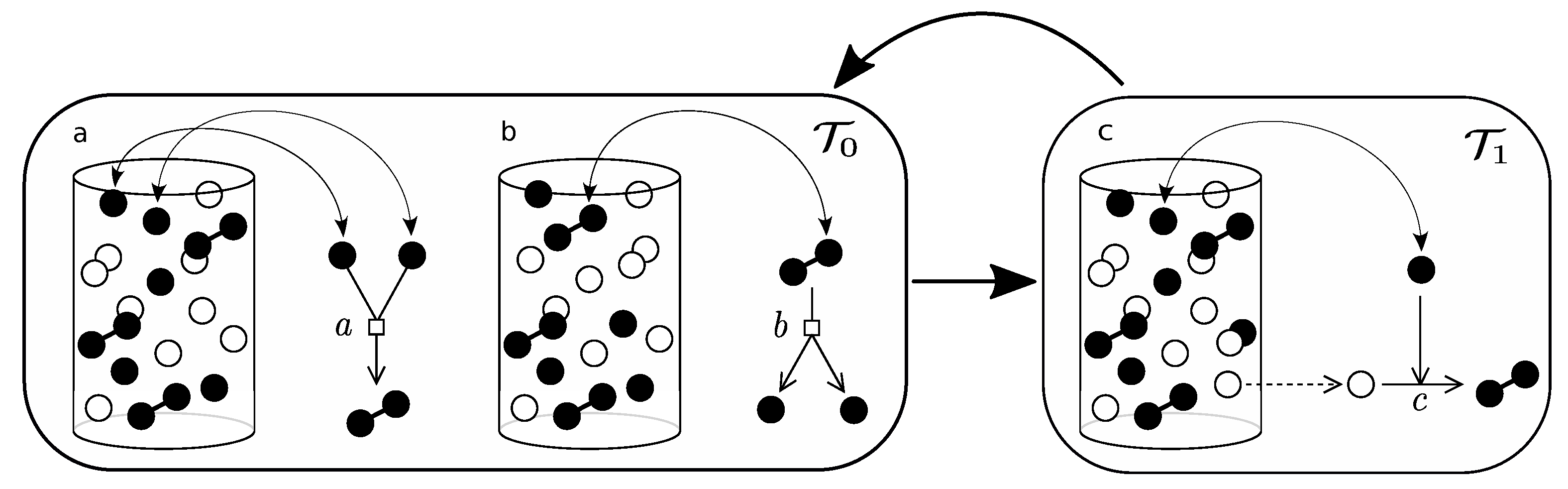
2.3. Coarse-Grained Dynamics of Replicators
- —state in which the system contains a total number of active chains.
- —state in which the system contains a total amount of n active chains.
3. Discussion
Acknowledgments
Author Contributions
Conflicts of Interest
Abbreviations
| MDPI | Multidisciplinary Digital Publishing Institute |
| DOAJ | Directory of open access journals |
| ESL | Extended Second Law |
| LEB | Lower Entropic Bound |
| LHS | Left Hand Side |
| RHS | Right Hand Side |
Appendix A
Appendix B
Appendix B.1
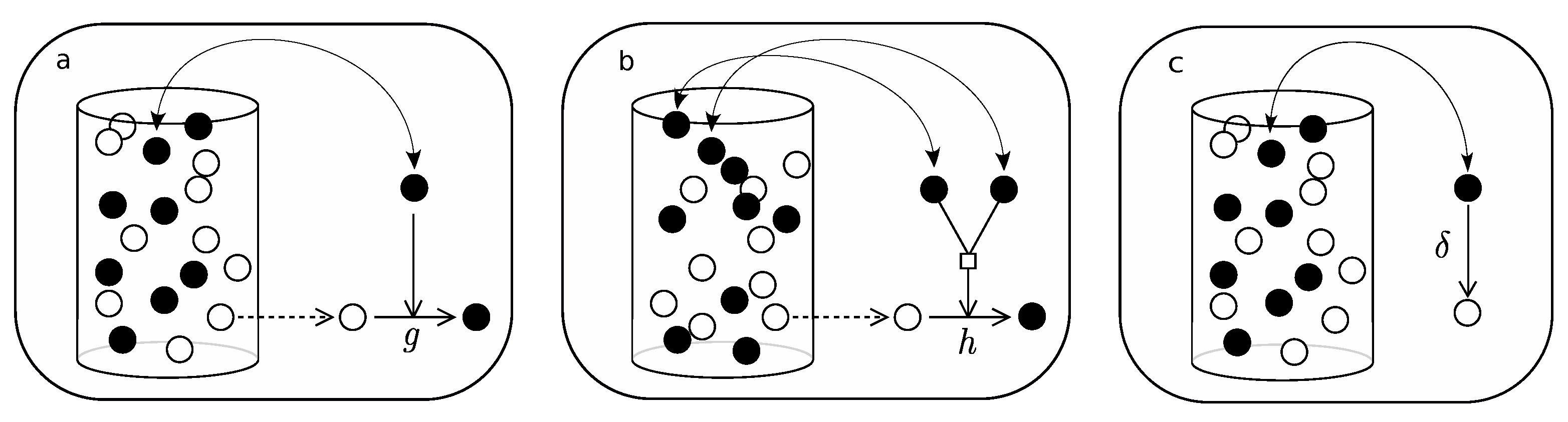
- Pick an element of the urn at random.
- If active, with probability g, pick a second element at random and (if not active) activate.
- Pick an element at random again.
- If active, with probability , deactivate.
Appendix B.2
- Pick an element of the urn at random.
- If active, pick a second element at random.
- If active, with probability h, pick a third element at random and (if not active) activate.
- Pick an element at random again.
- If active, with probability , deactivate.
Appendix B.3
- Pick an element of the urn at random. If active, then: (i) if in associated state () then, with probability a, dissociate and iterate; (ii) if dissociated, pick a second element and, if active, with probability b, associate. Iterate this process until equilibrium is reached for association/dissociation reaction.
- Pick an element of the urn at random. If active, pick a second element at random, if empty, with probability c, replicate.
- Pick an element of the urn at random. If active, with probability , deactivate.

References
- Hopfield, J.J. Physics, computation, and why biology looks so different. J. Theor. Biol. 1994, 171, 53–60. [Google Scholar] [CrossRef]
- Maynard-Smith, J.; Szathmáry, E. The Origins of Life; Oxford University Press: Oxford, UK, 1999. [Google Scholar]
- Dyson, F. Origins of Life; Cambridge University Press: Cambridge, UK, 1999. [Google Scholar]
- Kauffman, S.A. The Origins of Order: Self-Organization and Selection in Evolution; Oxford University Press: New York, NY, USA, 1993. [Google Scholar]
- Hofbauer, J.; Sigmund, K. Evolutionary Games and Population Dynamics; Cambridge University Press: Cambridge, UK, 1998. [Google Scholar]
- Morowitz, H.; Smith, E. The Origin and Nature of Life on Earth: The Emergence of the Fourth Geosphere; Cambridge University Press: Cambridge, UK, 2016. [Google Scholar]
- Kauffman, S.A. Investigations; Oxford University Press: New York, NY, USA, 2000. [Google Scholar]
- Babloyantz, A. Molecules, Dynamics and Life: An Introduction to Self-Organization of Matter; John Wiley & Sons: New York, NY, USA, 1986. [Google Scholar]
- Nicolis, G.; Prigogine, I. Exploring Complexity: An Introduction; W.H.Freeman & Co, Ltd.: New York, NY, USA, 1989. [Google Scholar]
- Glansdorff, P.; Prigogine, I. Thermodynamic Theory of Structure, Stability and Fluctuations; John Wiley & Sons, Ltd.: London, UK, 1971. [Google Scholar]
- Wagensberg, J. Complexity versus uncertiainty: The question of staying alive. Biol. Philos. 2000, 15, 493–508. [Google Scholar] [CrossRef]
- Jarzynksi, C. Nonequilibrium equality for free energy differences. Phys. Rev. Lett. 1997, 78, 2690–2693. [Google Scholar]
- Crooks, G.E. Nonequilibrium measurements of free energy differences for microscopically reversible Markovian systems. J. Stat. Phys. 1998, 90, 1481–1487. [Google Scholar] [CrossRef]
- Crooks, G.E. Entropy production fluctuation theorem and the nonequilibrium work relation for free energy differences. Phys. Rev. E 1999, 60, 2721–2726. [Google Scholar] [CrossRef]
- Gomez-Marin, A.; Parrondo, J.M.R.; van den Broeck, C. Lower bounds on dissipation upon coarse graining. Phys. Rev. E 2008, 78, 011107. [Google Scholar] [CrossRef] [PubMed]
- Still, S.; Sivak, D.A.; Bell, A.J.; Crooks, G.E. Thermodynamics of prediction. Phys. Rev. Lett. 2012, 109, 120604. [Google Scholar] [CrossRef] [PubMed]
- England, J. Statistical physics of self-replication. J. Chem. Phys. 2013, 139, 121923. [Google Scholar] [CrossRef] [PubMed]
- Perunov, N.; Marsland, R.A.; England, J. Statistical physics of adaptation. Phys. Rev. X 2016, 6, 021036. [Google Scholar] [CrossRef]
- Bartolotta, A.; Carroll, S.M.; Leichenauer, S.; Pollack, J. Bayesian second law of thermodynamics. Phys. Rev. E 2016, 94, 022102. [Google Scholar] [CrossRef] [PubMed]
- Szathmáry, E. The origin of replicators and reproducers. Philos. Trans. R. Soc. B 2006, 361, 1761–1776. [Google Scholar] [CrossRef] [PubMed]
- Szathmáry, E. From replicators to reproducers: The first major transitions leading to life. J. Theor. Biol. 1997, 187, 555–571. [Google Scholar] [CrossRef] [PubMed]
- Solé, R. Synthetic transitions: Towards a new synthesis. Philos. Trans. R. Soc. B 2016, 371, 20150438. [Google Scholar] [CrossRef] [PubMed]
- Eigen, M.; Schuster, P. The Hypercycle: A Principle of Natural Self-Organization; Springer: Berlin, Germany, 1979. [Google Scholar]
- Szathmáry, E.; Gladkih, I. Sub-exponential growth and coexistence of non-enzymatically replicating templates. J. Theor. Biol. 1989, 138, 55–58. [Google Scholar] [CrossRef]
- Scheuring, I.; Szathmáry, E. Survival of replicators with parabolic growth tendency and exponential decay. J. Theor. Biol. 2001, 212, 99–105. [Google Scholar] [CrossRef] [PubMed]
- Ellington, A.D. Origins for everyone. Evol. Educ. Outreach 2012, 5, 361–366. [Google Scholar] [CrossRef]
- Landauer, R. Irreversibility and heat generation in the computing process. IBM J. Res. Dev. 1961, 5, 183–191. [Google Scholar] [CrossRef]
- Bennett, C.H. The thermodynamics of computation—A review. Int. J. Theor. Phys. 1982, 21, 905–940. [Google Scholar] [CrossRef]
- Parrondo, J.M.R.; Horowitz, J.M.; Sagawa, T. Thermodynamics of information. Nat. Phys. 2015, 11, 131–139. [Google Scholar] [CrossRef]
- Zwanzig, R.W. High-temperature equation of state by a perturbation method. I. Nonpolar gases. J. Chem. Phys. 1954, 22, 1420–1426. [Google Scholar] [CrossRef]
- Szathmáry, E. Simple growth laws and selection consequences. Trends Ecol. Evol. 1991, 6, 366–370. [Google Scholar] [CrossRef]
- Maynard-Smith, J.; Szathmáry, E. The Major Transitions in Evolution; Oxford University Press: Oxford, UK, 1995. [Google Scholar]
- Eigen, M. Self-organization of matter and the evolution of biological macromolecules. Naturwissenchaften 1971, 58, 465–523. [Google Scholar] [CrossRef]
- Eigen, M.; Schuster, P. The hypercycle: A principle of natural self-organization. Part A: Emergence of the hypercycle. Naturwissenchaften 1977, 64, 541–565. [Google Scholar] [CrossRef]
- Eigen, M.; Schuster, P. The hypercycle: A principle of natural self-organization. Part B: The abstract hypercycle. Naturwissenchaften 1977, 65, 7–41. [Google Scholar] [CrossRef]
- Eigen, M.; Schuster, P. The hypercycle: A principle of natural self-organization. Part C: The realistic hypercycle. Naturwissenchaften 1977, 65, 341–369. [Google Scholar] [CrossRef]
- Vaidya, N.; Manapat, M.L.; Chen, I.A.; Xulvi-Brunet, R.; Hayden, E.J.; Lehman, N. Spontaneous network formation among cooperative RNA replicators. Nature 2012, 491, 72–77. [Google Scholar] [CrossRef] [PubMed]
- Lee, D.H.; Granja, J.R.; Martinez, J.A.; Severin, K.; Ghadiri, M.R. A self-replicating peptide. Nature 1996, 382, 525–528. [Google Scholar]
- von Kiedrowski, G. A self-replicating, hexadeoxy nucleotide. Angew. Chem. Int. Ed. Engl. 1986, 25, 932–935. [Google Scholar] [CrossRef]
- Zielinski, W.S.; Orgel, L.E. Autocatalytic synthesis of a tetranucleotide analogue. Nature 1977, 327, 346–347. [Google Scholar] [CrossRef] [PubMed]
- Paul, N.; Joyce, G.F. Minimal self-replicating systems. Curr. Opin. Chem. Biol. 2004, 8, 634–639. [Google Scholar] [CrossRef] [PubMed]
- Méndez, V.; Campos, D.; Bartumeus, F. Stochastic Foundations in Movement Ecology: Anomalous Diffusion, Front Propagation and Random Searches; Springer: Heidelberg, Germany, 2014. [Google Scholar]
- Redner, S. A Guide to First-Passage Processes; Cambridge University Press: Cambridge, UK, 2001. [Google Scholar]
- von Neumann, J.; Burks, A.W. Theory of Self-Reproducing Automata; University of Illinois Press: Urbana, IL, USA, 1966. [Google Scholar]
- Sipper, M.; Reggia, J.A. Go forth and replicate. Sci. Am. 2008, 18, 48–57. [Google Scholar] [CrossRef]
- Andrieux, D.; Gaspard, P. Nonequilibrium generation of information in copolymerization processes. Proc. Natl. Acad. Sci. USA 2008, 105, 9516–9521. [Google Scholar] [CrossRef] [PubMed]
- Ouldridge, T.E.; ten Wolde, P.R. Fundamental costs in the production and destruction of persistent polymer copies. Phys. Rev. Lett. 2017, 118, 158103. [Google Scholar] [CrossRef] [PubMed]
- Griffith, E.C.; Tuck, A.F.; Vaida, V. Ocean-atmosphere interactions in the emergence of complexity in simple chemical systems. Acc. Chem. Res. 2012, 45, 2106–2113. [Google Scholar] [CrossRef] [PubMed]
- García-Tejedor, A.; Castaño, A.R.; Morán, F.; Montero, F. Studies on evolutioanry and selective properties of hypercycles using a Monte Carlo method. J. Mol. Evol. 1987, 26, 294–300. [Google Scholar]
- García-Tejedor, A.; Sanz-Nuño, J.C.; Olarrea, J.; de la Rubia, F.J.; Montero, F. Influence of the hypercyclic organization on the error threshold: A stochastic approach. J. Theor. Biol. 1988, 134, 431–443. [Google Scholar]


| Replicator Class | Reaction Scheme | Effective Dynamics |
|---|---|---|
| Simple | ||
| Hyperbolic | ||
| Parabolic |
© 2018 by the authors. Licensee MDPI, Basel, Switzerland. This article is an open access article distributed under the terms and conditions of the Creative Commons Attribution (CC BY) license (http://creativecommons.org/licenses/by/4.0/).
Share and Cite
Piñero, J.; Solé, R. Nonequilibrium Entropic Bounds for Darwinian Replicators. Entropy 2018, 20, 98. https://doi.org/10.3390/e20020098
Piñero J, Solé R. Nonequilibrium Entropic Bounds for Darwinian Replicators. Entropy. 2018; 20(2):98. https://doi.org/10.3390/e20020098
Chicago/Turabian StylePiñero, Jordi, and Ricard Solé. 2018. "Nonequilibrium Entropic Bounds for Darwinian Replicators" Entropy 20, no. 2: 98. https://doi.org/10.3390/e20020098
APA StylePiñero, J., & Solé, R. (2018). Nonequilibrium Entropic Bounds for Darwinian Replicators. Entropy, 20(2), 98. https://doi.org/10.3390/e20020098