Article

Entropy Generation Rates through the Dissipation of Ordered Regions in Helium Boundary-Layer Flows

by
LaVar King Isaacson
Department of Mechanical Engineering, University of Utah, Salt Lake City, UT 84112, USA
Entropy 2017, 19(6), 278; https://doi.org/10.3390/e19060278
Submission received: 23 March 2017 / Revised: 9 June 2017 / Accepted: 12 June 2017 / Published: 15 June 2017
(This article belongs to the Special Issue Entropy in Computational Fluid Dynamics)

Abstract

:
The results of the computation of entropy generation rates through the dissipation of ordered regions within selected helium boundary layer flows are presented. Entropy generation rates in helium boundary layer flows for five cases of increasing temperature and pressure are considered. The basic format of a turbulent spot is used as the flow model. Statistical processing of the time-dependent series solutions of the nonlinear, coupled Lorenz-type differential equations for the spectral velocity wave components in the three-dimensional boundary layer configuration yields the local volumetric entropy generation rates. Extension of the computational method to the transition from laminar to fully turbulent flow is discussed.

1. Introduction

This article presents the results of the computation of the entropy generation rates occurring through the dissipation of ordered regions in the nonlinear time series solutions of the fluctuating spectral velocity wave vector equations for several helium boundary layer environments. These equations are cast in a Lorenz format and solved with the three-dimensional helium boundary layer profiles as input parameters. The computational procedures employed for these calculations have been presented previously in Isaacson [1,2]. This article follows closely the format of [2], indicating the major mathematical equations used in the computational procedures. The purpose of this approach is to provide the reader the opportunity to follow the equations as they are presented, rather than requiring a continuous reference to previous literature.
The computational procedure used for the studies reported in [1,2] consists of two fundamental thermodynamic components. The first component, classified as the thermodynamic reservoir, is made up of the three-dimensional steady laminar boundary layer velocity profiles in the x–y and the z–y planes of the flow. This thermodynamic reservoir provides the steady state velocity gradients in the x–y and the z–y planes that serve as input control parameters for the second thermodynamic component, the time-dependent subsystem producing the nonlinear flow instabilities within the boundary layer. The second thermodynamic system, the time dependent subsystem, includes the set of equations describing the development of the spectral wave components and the set of coupled, nonlinear equations describing the development of the spectral velocity wave components with time. The set of equations describing the nonlinear time development of the spectral velocity wave components are cast into a Lorenz-type format that is sensitive to the initial conditions applied to the integration of the equations. The steady state boundary layer velocity gradients serve as control parameters for these equations and are determined by the particular value of the kinematic viscosity for the system. While the control parameters are obtained from the steady state boundary layer solutions, which are controlled by the kinematic viscosity, the initial conditions for the integration of the Lorenz-type equations are dependent upon the turbulence levels imposed on the system from the free stream. Walsh and Hernon [3] have presented experimental measurements of the unsteady fluctuation levels in laminar boundary layers when subjected to free stream turbulence. These measurements indicate that the free stream turbulence level must be taken into account when computing the entropy generation rates in three-dimensional boundary layers. We have accounted for the free stream turbulence level by choosing the initial conditions applied to the time integration of the modified Lorenz equations for the nonlinear solutions for the spectral velocity wave components.
Isaacson [1] presents computational results for the entropy generation rates through the dissipation of ordered regions in an air boundary layer with crosswind velocities at a temperature of 1068.0 K and a pressure of 0.912 × 10⁵ N/m2 at a normalize vertical location of η = 3.00 (see Equation (5) for the definition of η). The kinematic viscosity for air at these conditions is ν = 1.51634 × 10⁻⁴ m2/s. Isaacson [2] presents similar results for the laminar boundary-layer layer, also with a crosswind velocity, at a normalized vertical location of η = 1.40, with the same value of kinematic viscosity.
The results presented in [1,2] also indicate that instabilities are produced for this value of kinematic viscosity at these two vertical locations for several stations along the stream wise laminar boundary layer development. Thus, the generation of these instabilities has the general configuration of the formation of turbulent spots within the three-dimensional boundary layer flow environment. Boiko et al. [4] report the experimentally observed development of two turbulent spots measured within the boundary layer, thus validating the predicted general configuration of the instabilities as the development of turbulent spots.
It has been noted in [1,2] that instabilities are predicted for a narrow range of kinematic viscosities, namely, for ν = 1.5 × 10⁻⁴ m2/s to ν = 1.6 × 10⁻⁴ m2/s. The value of the kinematic viscosity applied to the solution of the steady three-dimensional boundary layer equations for the velocity gradient control parameters in the primary thermodynamic reservoir determines the values for these particular control parameters. It is thus of fundamental engineering interest that helium, with a very low density, has kinematic viscosities in this range over a considerable variety of temperatures and pressures. The values for the kinematic viscosities of helium for a selection of temperatures and pressures are given in Table 1. We have applied our computational procedure to engineering flow systems that use helium in a three-dimensional flow configuration for this set of values of kinematic viscosity.
A significant component in Generation IV Nuclear Energy Systems is dependent on the further development of the Helium Brayton Cycle with Interstage Heating and Cooling [5]. It is therefore prudent to explore areas of entropy production in helium flow systems with the objective of improving the overall thermal efficiencies of these systems.
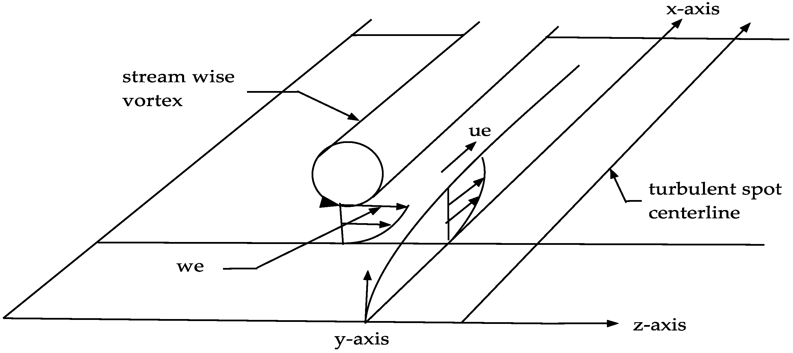
The flow configuration modeled in this study is that of the initial formation of a turbulent spot within the laminar flow as shown in Figure 1. This configuration is discussed in detail in Schmid and Henningson [6] and Belotserkovskii and Khlopkov [7]. The flow consists essentially of two counter rotating stream wise vortices which meet at a point in the downstream direction, thus forming the shape of an arrow, with the tip pointing in the downstream direction. Between the two vortices, a stream wise laminar boundary layer is formed along the flow surface. We model only the left hand side configuration, consisting of a counter-clockwise rotating vortex interacting with the stream wise laminar boundary layer flow.
This article includes the following sections: in Section 2, the thermodynamic and transport processes of the working substance required for the computational procedures are discussed. In this study, the working substance is the flow of a helium mixture at five sets of specified temperature and pressure. In Section 3, the mathematical and computational bases for the evaluation of the steady three-dimensional boundary layer environment are reviewed. In Section 4, the fluctuation equations of Townsend [8] and Hellberg and Orszag [9] are transformed into the spectral plane and written in the Lorenz format. 
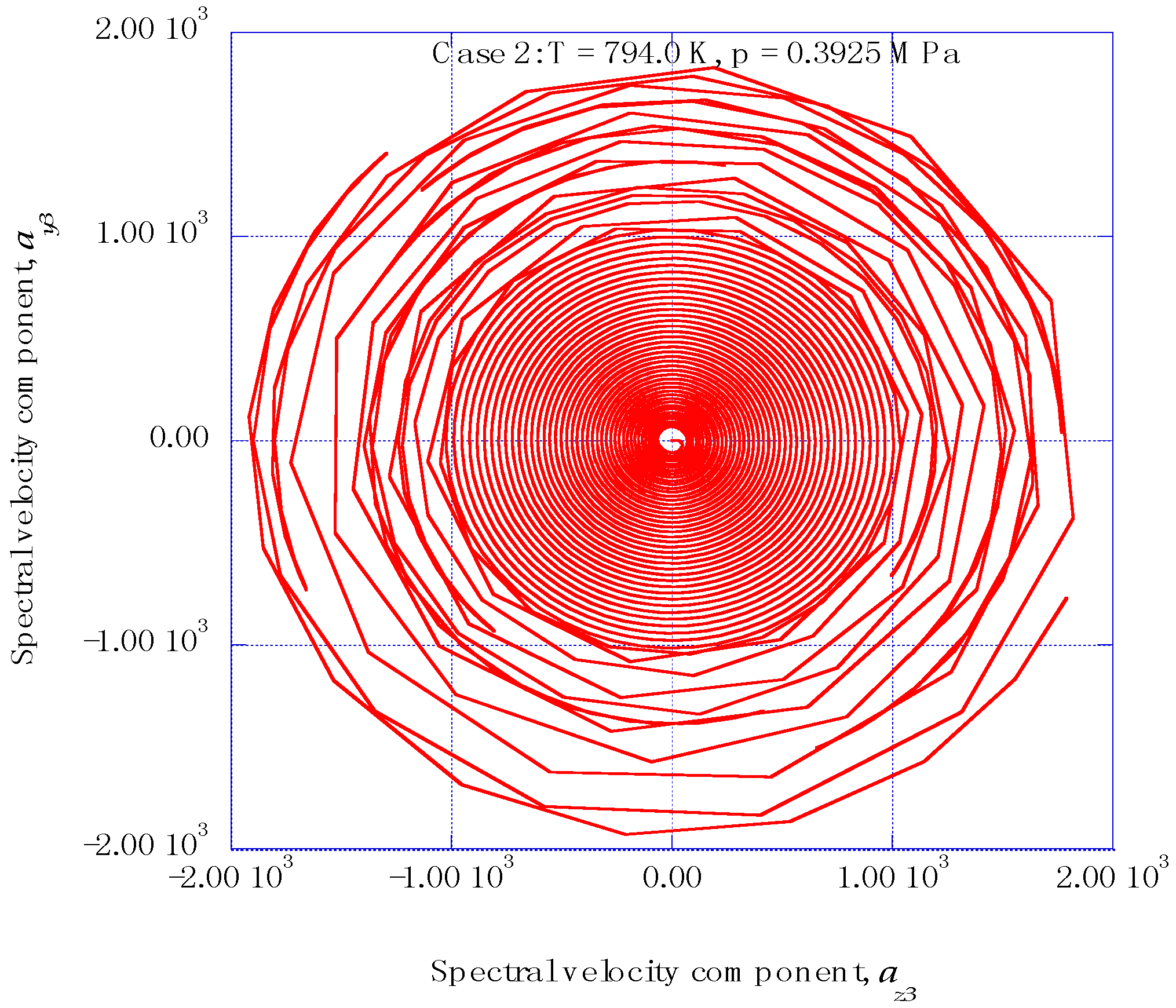
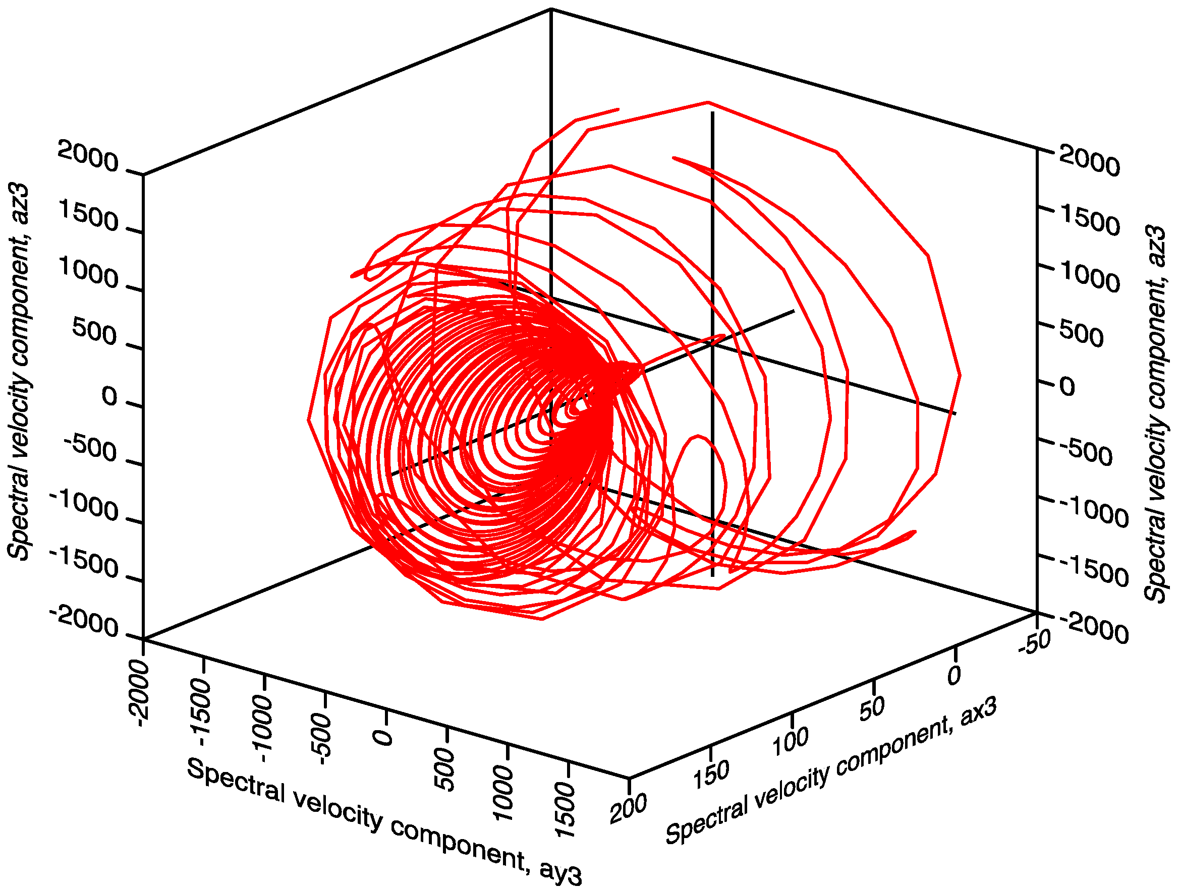
Section 5 presents computational results for the time-dependent spectral velocity components for a temperature of 794.0 K and a pressure of 0.3925 MPa. Section 6 discusses the extraction of empirical entropies, empirical entropic indices, and intermittency exponents from the nonlinear time series solutions of the modified Lorenz equations. Section 7 includes a comparison of the entropy generation rate for each of the five sets of temperature and pressure for the normalized vertical location of η = 3.00 and the stream wise distance of x = 0.120 with the entropy generated across a corresponding turbulent boundary layer. The article closes with a discussion of the results and final conclusions.

2. Selection of Helium as the Working Substance

We consider five special cases of thermodynamic and transport properties for the helium working gas. The first case is the development of flow instabilities for helium boundary layers at atmospheric pressure and corresponding temperature. The second case models the temperature and pressure values that occur at several key locations in the Generation IV Nuclear Helium Brayton Cycle with Interstage Heating and Cooling Concept [5]. The third, fourth and fifth cases consider higher temperature and pressure values that also occur in Generation IV Nuclear Energy Systems [5].
The working gas is assumed to be a mixture of helium together with small amounts of other gases. The composition of the working gas is as follows: 99.96 percent helium; 0.01 percent argon; 0.01 percent nitric oxide; 0.01 percent oxygen; 0.01 percent nitrogen. The purpose of including other species in addition to helium in the working gas is to more closely approximate an actual gaseous environment that includes impurities. The thermodynamic and transport properties of this mixture for each of the five cases considered in the study are listed in Table 1.
To compute the generation of boundary layer instabilities, a series of coupled, nonlinear time-dependent differential equations are included in the computational procedure. The solutions for such equations are sensitive to the initial conditions imposed on the equations and also depend on the control parameters applied in the solutions. The solutions of the steady-state boundary-layer equations that provide these control parameters are dependent on the particular values of the kinematic viscosity applied in the calculations. Using the same initial conditions as applied in the study reported here, a series of values for the kinematic viscosity were found, outside the range indicated in Table 1, that also indicate the generation of instabilities within three-dimensional helium laminar boundary layer flows. Hence, the values of kinematic viscosities that predict three-dimensional boundary layer instabilities are not limited to the values listed in Table 1.

3. Steady-Flow Laminar Boundary-Layer Environment

This section presents a summary of the mathematical and computational methods used for the determination of the x–y plane and the z–y plane steady-state laminar boundary-layer velocity gradients. These boundary layer mean velocity gradients are time independent but vary with the stream wise distance x. The boundary-layer mean velocity gradients serve as control parameters for the solution of the time-dependent fluctuating spectral velocity equations, yielding the initiation of instabilities within the boundary layer for each stream wise station, as summarized in Section 4 of the article.
Singer [10] has reported the results of the direct numerical simulation of the development of a young turbulent spot in an incompressible constant-pressure boundary layer in a flow stream with strong free stream turbulence. These studies indicate the development of a counter-clockwise stream wise vortex flow that produces a viscous laminar boundary layer in the z–y plane of the flow environment as shown in Figure 1. Ersoy and Walker [11] discuss the development of this z–y plane boundary layer produced by the interaction of the vortex tangential velocity with the flow surface. The stream wise flow along the flow surface in the central region of the turbulent spot produces a laminar boundary layer flow along the surface in the x–y plane of the flow configuration, also shown in Figure 1.
Cebeci and Bradshaw [12] and Cebeci and Cousteix [13] provide computer source code listings that we have used to compute the laminar boundary layer velocity profiles for both the x–y plane and the z–y plane. Hansen [14] has shown that these orthogonal profiles are similar in nature and thus allow the simultaneous use of these profiles in our three-dimensional flow computations.
The steady three-dimensional boundary layer solutions are obtained for a sequence of stations along the x-axis. These solutions provide the profiles of the respective steady state boundary layer velocity gradients. These steady boundary layer velocity gradients serve as control parameters for the solutions of both the spectral wave component equations and the fluctuating spectral velocity wave component equations. 
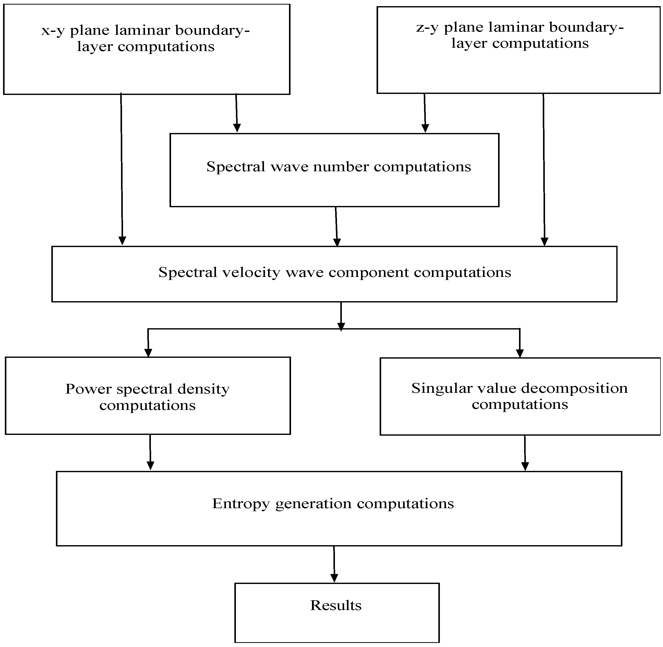
Figure 2 shows a flow chart of the sequence of computational procedures from the solution of the steady boundary layer equations to the final computation of the entropy generation rates [1]. Each of the computational procedures shown Figure 2 is discussed in following sections.
There are three fundamental objectives in presenting the classical transformation of the boundary layer equations to the form employed for integration. First, the Falkner–Skan transformation method provides three, first-order, differential equations which are solved with the Keller–Cebeci Box method yielding the steady boundary-layer velocity profiles, either for a laminar boundary layer or a turbulent boundary layer. Second, these first-order equations are extended to the evaluation of the mean boundary-layer velocity gradients [15] that serve as the control parameters for the time-dependent Lorenz-type equations for the computations of the instabilities produced by the interactions of the z–y velocity gradients with the x–y boundary layer gradients. The third objective is to obtain velocity gradient values for the laminar case of entropy generation rates from Equation (40) and turbulent velocity gradients for the prediction of the entropy generation rates in turbulent boundary layers from Equation (45).
The boundary-layer configuration considered in this article consists of a laminar boundary layer in the x–y plane produced by the stream wise velocity along the horizontal surface and a laminar boundary layer in the z–y plane produced by the vortex tangential edge velocity in the z-direction. The momentum equation for the thin-shear boundary layer approximation may be written [12] as:
u u x + v u y = 1 ρ d p d x + 1 ρ y [ μ u y ρ u v ¯ ] .
The boundary conditions for Equation (1) are:
y = 0 ,   u = v = 0 ,
y = δ ( x ) ,   u = u e ( x )
The Reynolds shear stress for the computation of turbulent boundary layers is modeled with the “eddy viscosity”, εm, having the dimensions of (viscosity)/(density), by:
ρ u v ¯ = ρ ε m u y
The computer program we have chosen to implement for the solution of the boundary layer equation (Equation (1)) is based on the Keller–Cebeci Box method presented by Cebeci and Bradshaw [12] and Cebeci and Cousteix [13]. One of the basic aspects of this method is to transform Equation (1) into a system of first-order ordinary differential equations. The Falkner–Skan transformation, in the form:
η = ( u e ν x ) 1 / 2 y ,
is introduced into the transformation process. The dimensionless stream function, f(x,η), is defined by
Ψ ( x , y ) = ( u e ν x ) 1 / 2 f ( x , η ) .
These definitions yield the results for the mean boundary layer velocities u and v as
u = u e f , v =   x [ ( u e ν x ) 1 / 2 f ] + η 2 ( u e ν x ) 1 / 2 f .
Differentiation with respect to η is indicated by the prime in these expressions.
From Bernoulli’s equation, the pressure gradient term is given by d p d x = ρ u e d u e d x . To simplify the resulting equations, the parameter m is defined as:
m = x u e d u e d x
Applying these transformations, the momentum equation for the boundary layer (Equation (1)) becomes:
( ( 1 + ε m ν ) f ) + m + 1 2 f f + m [ 1 ( f ) 2 ] = x ( f f x f f x ) ,
with boundary conditions:
f ( x , 0 ) = 0 ,
f ( x , 0 ) = 0 ,   lim η f ( x , η ) = 1
The computer solution procedures for this third-order differential equation, as developed by Cebeci and Bradshaw [12], replace the third-order differential equation, Equation (9), with three first-order differential equations in the following fashion:
f = u ,
u = v ,
( ( 1 + ε m ν ) v ) + ( m + 1 2 ) f v + m ( 1 u 2 ) = x ( u u x v f x )
The corresponding boundary conditions for these equations are:
f(x,0) = 0,   u(x,0) = 0,   u(x,η) = 1.
Note that in Equation (13), v is not the y-component velocity.
Cebeci and Bradshaw [12] present computer program listings for the numerical solutions for both laminar and turbulent boundary layers over flat plate surfaces. The program listings used in the study reported here are those presented in [12].
Hansen [14] has indicated that orthogonal laminar boundary layer profiles in a three-dimensional coordinate system possess the characteristic of similarity. We therefore use the boundary layer computations for both the profiles in the x–y plane and in the z–y plane. The steady state boundary layer equations and the corresponding velocity gradients serve as the thermodynamic steady state reservoir that provides the control parameters for the time-dependent development of the spectral fluctuations within the boundary layer environment [16].

4. Modified Time-Dependent Lorenz Equations in the Spectral Plane

4.1. Transformation of the Townsend Equations to the Modified Lorenz Format

The methods of Townsend [8] are used to obtain a set of non-equilibrium, time-dependent equations in the spectral domain for these non-equilibrium instabilities, separate from the equations for the steady boundary layer flow. The time-dependent spectral equations of Townsend [8] and Hellberg et al. [9] are embedded into the computational results obtained from the steady boundary layer solutions for the steady state boundary layer velocity profiles. These non-equilibrium spectral equations are cast into a Lorenz format [17] to yield the nonlinear time series solutions for the fluctuating components of the spectral velocity field.
The nonlinear time series solutions of the modified Lorenz equations yield both smooth trajectories and trajectories with fluctuating spectral velocity components within the series. Statistical analysis of the fluctuating spectral time-series solutions yields the entropy generation rates for the given flow configurations. The correspondence of the peaks of the spectral power density analysis and the empirical modes of the singular value decomposition analysis is brought about by the Weiner–Khintchine theorem relating the power density spectrum and the autocorrelation function for the nonlinear time series data [16].
Separating the equations of motion into steady and unsteady equations, the equations for the velocity fluctuations may then be written as [13,14]:
u i t + U j u i x j + u j U i x j + u j u i x j = 1 ρ p x i + ν 2 u i u j u j
In these equations, ρ is the density and ν is the kinematic viscosity, Ui represent the mean boundary layer velocity components with i = 1, 2, 3 indicating the x, y, and z components, and xj, with j = 1, 2, 3, designate the x, y and z directions. The pressure term is eliminated by taking the divergence of Equation (16) and invoking incompressibility, yielding:
1 ρ 2 p x l 2 = 2 U l x m u m x l + u l x m u m x l .
We wish to transform these equations into the spectral plane for the computational solutions for the time-dependent fluctuating spectral components. The solutions of the spectral equations yield the spectral wave vector components and the spectral velocity wave components. Through Parseval’s theorem, the products of the spectral velocity components represent the products of the fluctuating velocity components in the physical plane. The statistical analysis of the spectral velocity component time series solutions then yields the entropy generation rates within the boundary layer non-equilibrium ordered regions.
The fluctuating velocity and pressure fields of Equations (16) and (17) may be expanded in terms of the Fourier components [18] as:
u i ( x , t ) = k a i ( k , t ) exp ( i k x ) ,
and:
p ( x , t ) ρ = k b ( k , t ) exp ( i k x ) .
The pressure component in Equation (16) is transformed into a function of spectral velocity components and boundary layer velocity gradients through Equations (18) and (19). Substituting the resulting equations and Equation (18) into Equation (16) yields an expression for the fluctuations of the spectral components with time. The equations for the time-dependent three spectral velocity wave components, ai(k), are then given as [8]:
d a i ( k ) d t = ν k 2 a i ( k ) U i x i a i ( k ) + 2 k i k l k 2 U l x m a i ( k ) + i k + k = k ( k l k i k m k 2 δ i m k l ) a l ( k ) a m ( k ) .
The general equations for the balance of transferable properties give the equations for the spectral wave numbers, ki as:
d k i d t = U l x i k l .
The set of equations for the time-dependent wave number components, including the gradients of the mean velocities in the x–y and z–y boundary layers, may be written:
d k x d t = U x k x V x x k y ,
d k y d t = U y k x V x y k y W y k z ,
d k z d t = V z z k y W z k z .
The nonlinear products of the spectral velocity components in Equations (20) are retained in our series of equations by characterizing the coefficients:
k l ( δ i m k i k m k 2 ) ,
as a projection matrix [18]. This coefficient represents the projection of a given velocity wave vector component, ai, normal to the direction of the corresponding wave number component, ki. A model equation for this expression in the form:
1 − K * cos(k(t)),
is introduced to retain the effect of the projection matrix on the nonlinear interactive terms in our equations. K is an empirical weighting amplitude factor [19] and k(t) is given by:
k ( t ) = ( k x 2 ) .
With F = Kcos(k(t)), the equations for the spectral velocity components, Equations (20), are written in Lorenz format as [15]:
d a x n d t = σ y n a y n σ x n a x n
d a y n d t = ( 1 F ) a r n a z n + r n a x n s n a y n ,
d a r n d t = ( 1 F ) a r n a y n b n a z n
From Equations (20), the coefficients of the velocity wave component terms have the following forms [15]:
σ y n = [ ( 2 k x k x k 2 1 ) U y + 2 k x k y k 2 V x y + 2 k x k z k 2 W y ] ,
σ x n = { ν k 2 [ ( 2 k x k x k 2 1 ) U x + 2 k x k y k 2 V x x + 2 k x k z k 2 W x ] } ,
r n = [ 2 k y k x k 2 U x + ( 2 k y k y k 2 1 ) V x x + 2 k y k z k 2 W x ] ,
s n = { ν k 2 [ 2 k y k x k 2 U y + ( 2 k y k y k 2 1 ) V z y + 2 k y k z k 2 W y ] } ,
b n = { ν k 2 [ 2 k z k x k 2 U z + 2 k z k y k 2 V z z + ( 2 k z k z k 2 1 ) W z ] } .
The nonlinear time series solutions for the spectral velocity wave number components in the spectral domain for each of the six downstream stations make up the non-equilibrium thermodynamic system. Solutions of the overall set of equations are obtained at each of the six stations along the x-axis.
The application of these equations at the initial station requires that additional assumptions be applied to the modified Lorenz equations. Isaacson [15], Mathieu and Scott [18], and Manneville [20] have discussed both the format and justification for the particular choice of these assumptions for the initial station. These solutions contain the spectral velocity component fluctuations that we wish to study.

4.2. Sensitivity to Initial Conditions and the Concept of Receptivity

The free stream velocity for the stream wise boundary layer flow is taken as a constant, ue = 1.00 [12] while the vortex tangential velocity is we = 0.08 [7]. The solutions of the steady boundary layer velocity gradient profiles in the x–y plane and the z–y plane provide the control parameters for the solutions of the modified Lorenz equations for the fluctuating spectral velocity wave equations. The solutions of Equations (28)–(30) yield the fluctuating spectral velocity wave components for the transmitter station at the stream wise location x = 0.060 and the span wise location of z = 0.003. The outer edge of the boundary layer is assumed to be at the normalized distance ηe = 8.00, with the boundary layer instability observed within the boundary layer at a normalized distance from the horizontal surface of approximately η = 3.0. For the kinematic viscosities given in Table 1, the weighting factor that yields flow instabilities has been found to be K = 0.05. The time step for the time-dependent integration process is taken as h = 0.0001 s.
Schmid and Henningson [6] discuss the concept of the receptivity of boundary layer flows to outside disturbances and the subsequent development of various instabilities that may occur in the boundary layer flow environment. The solutions of nonlinear, coupled differential equations such as the Lorenz equations are sensitive to the choice of the initial conditions. We have found consistent solutions with initial values for the spectral wave number equations of kx(1) = 0.04, ky(1) = 0.02 and kz(1) = 0.02.
A number of combinations of initial conditions have been applied for the solution of the spectral velocity wave equations. We have found that the initial conditions for the spectral velocity wave equations of ax(1) = 0.10, ay(1) = 0.04 and az(1) = 0.04 yield strong ordered regions in the time series solutions. These are the initial conditions used for the reported computed results for the modified Lorenz equations.
The initial conditions applied to the spectral velocity wave equations must arise from the external disturbances to the boundary layer flows. The incorporation of the time dependent spectral wave equations of the Lorenz format in the computational process may thus open the possibility of connecting the concept of boundary layer receptivity to the subsequent development of ordered regions in helium boundary layer flow environments.
We apply our computational procedure to the five stations following the initial station at x = 0.060 along the stream wise direction. However, as Attard [16] points out, we must take into account that the nonlinear time series solutions obtained for the second and subsequent stations will be influenced by the fluctuations produced in the first and following stations. To accomplish this, we use the synchronization properties of the modified Lorenz set of equations describing the nonlinear solutions for the spectral components [1,15].

4.3. Synchronization Properties of the Modified Lorenz Equations

Pecora and Carroll [21], Pérez and Cerdeiral [22], and Cuomo and Oppenheim [23] have used the synchronization properties of systems of Lorenz-type equations to extract messages masked by chaotic signals. The synchronization properties of Lorenz-type equations are adapted here to extract ordered signals from the nonlinear time series generated for each of the spectral components in the solutions of the modified Lorenz equations.
We apply the transformation of the projection matrix (Equation (26)) to the initial station at x = 0.060. We then apply the synchronization properties to each of the following downstream stations. The various boundary layer coefficients at each of these stations are computed in the same manner as in the initial station. Following the results in [15], the time-dependent output for the x-direction spectral velocity component from the initial station is used as input to the nonlinear coupled terms in the modified Lorenz equations at the next station, which we denote as the first station in the x-direction. Then, the input to the nonlinear-coupled terms at the next downstream station is made up of the sum of the stream wise velocity wave component output from the initial station plus the x-direction spectral velocity wave component output from the next downstream station. This process is repeated for each of the five downstream stations. With this method, the memory of the initial velocity fluctuations and the influence of subsequent fluctuations are retained in the overall computational procedure.

4.4. Deterministic Results for the Modified Lorenz Equations

We have obtained solutions for the fluctuating spectral velocity components for each of the five cases listed in Table 1 at six stream wise stations. We have chosen to present graphical results in Figure 3 through 8 for Case 2, with a temperature of T = 794.0 K and a pressure of p = 0.3925 MPa. These results indicate the clearest power spectral density peaks in the overall set of statistical results. Figure 3 shows the deterministic stream wise spectral velocity component, ax3, at the downstream station of x = 0.120, for a tangential vortex velocity of we = 0.080. Note that the subscript x3 represents the stream wise velocity component at the third receiver station in the x-direction. Figure 4 shows the corresponding phase diagram for ay3ax3, where ay3 is the normal spectral velocity wave component and az3 is the span wise spectral velocity wave component, again at the station x = 0.120.
Figure 5 shows the corresponding phase diagram for ay3az3, where az3 is the span wise spectral velocity wave component and ay3 is the normal spectral velocity wave component, again at the station x = 0.120. Figure 6 shows a three-dimensional representation of the deterministic trajectories of the three spectral velocity components for Case 2 for the stream wise station of x = 0.120 and the vortex tangential velocity of we = 0.08. These results indicate the formation of an initially strong spiral cone in the stream wise direction, transforming into a strongly oscillating motion in the span wise, normal planes of the flow environment. Our statistical analysis focuses on the fluctuating spectral velocities in the latter, strongly oscillating motion of the trajectories.

5. Ordered Regions within the Non-Equilibrium Spectral Velocity Time-Series Solutions

5.1. Power Spectral Densities Indicating Ordered Regions

The power spectral densities within the nonlinear time series solutions for the fluctuating spectral velocity components are computed using Burg’s method [24], providing the spectral peaks of the ordered regions within the time series solutions [19].
The Lorenz synchronization procedure yields the nonlinear time series solution for each of the five stations in the x-direction, following the initial station. These solutions indicate the generation of deterministic ordered regions, with significant non-equilibrium velocity fluctuations embedded within the solutions. Entropy generation comes about through the dissipation of these fluctuations into equilibrium thermodynamic states. We have found that Burg’s method [24] for the power spectral density of the time-series data is an effective method for extracting the underlying structural characteristics of the velocity fluctuations within the nonlinear time series solutions.
The resulting power spectral density results for the normal spectral velocity wave component, ay3 at the third receiver station at x = 0.120, are presented in Figure 7. For each of the power spectral density results, we have assigned empirical mode numbers to these peaks, starting with mode j = 1 representing the highest peak in the distribution, continuing to mode j = 16, representing the corresponding lowest peak among the sixteen peaks.
The peaks of the spectral power density analysis and the empirical modes of the singular value decomposition analysis are computed from the same set of time series data. Therefore, we can relate each power spectral density peak with a corresponding empirical mode through the Weiner–Khintchine theorem relating the power density spectrum and the autocorrelation function for the nonlinear time series data [16].
The results shown in Figure 7 for the power spectral density for the normal spectral velocity component indicate that the kinetic energy available for dissipation is distributed in well-defined spectral peaks or empirical modes. Simpson’s integration rule is used to obtain the kinetic energy within each mode, ξj, for each of the power spectral density empirical modes. The total kinetic energy contained within the ordered regions is then obtained as the sum of the individual contributions across the modes. This value is then used to get the fraction of kinetic energy in each mode that is available for dissipation into internal energy.

5.2. Empirical Entropies from Singular Value Decomposition

The singular value decomposition procedure [25] can also serve as a means of identifying fundamental characteristics of the nonlinear time series solutions of the coupled nonlinear spectral equations. We have incorporated into our numerical procedure the singular value decomposition computer program listings presented by Press et al. [19]. The computational procedure is made up of two parts, the computation of the autocorrelation matrix and the singular value decomposition of that matrix [19]. The overall computational procedure yields the empirical eigenvalues for each of the empirical eigenfunctions for the given nonlinear time series data segment.
The application of the singular value decomposition procedure to a specified segment of the nonlinear time-series solution for each of the spectral velocity wave components yields the distribution of the component eigenvalues λj across the empirical modes, j, for each of the flow conditions listed in Table 1. The empirical entropy, Sempj, is defined from these eigenvalues by the expression [26]:
S e m p j = ln ( λ j ) .
Here, λj is the empirical eigenvalue computed from the singular value decomposition procedure applied to the nonlinear time-series solution. The distribution of the empirical entropy across the decomposition empirical modes has been shown in [15]. We have applied the singular value decomposition procedure to the nonlinear time-series solutions of the modified Lorenz non-equilibrium equations.

5.3. Empirical Entropic Indices for the Ordered Regions

The results indicate that the majority of the kinetic energy is contained within the first seven empirical modes of the singular value decompositions, with relatively low empirical entropy. The following three empirical modes indicate a transition into non-equilibrium ordered regions. These regions have been classified as coherent [25] with well-defined structural boundaries. We wish to find a way to follow these regions through the process of transition from ordered regions into equilibrium thermodynamic states. For this, we turn to the concept of the Tsallis entropic format [27].
The Tsallis entropic format is applicable to a variety of microscopic and macroscopic sub-systems. We are working with a collection of statistical sub-systems spread over a limited number of empirical modes, j. Note that this is not a sequence over time, but is a sequence in phase space [16]. The empirical entropy, Sempj is introduced to describe the entropy of an ordered region described by the empirical eigenvalue, λj, for the singular value decomposition empirical mode, j. Hence, we simply adopt, in an ad hoc fashion, an expression from which we may extract an empirical entropic index, qj, from the empirical entropy, Sempj. This expression is written as [15]:
S e m p j = ln ( λ j ) = ( λ j ) q j 1 ( 1 q j ) .
This expression includes the effects of the nonlinear, non-equilibrium nature of the ordered regions we are following. It has the format of an entropic index; hence, we simply call qj the empirical entropic index or simply the entropic index for the empirical mode, j. The empirical entropic indices for the normal spectral velocity wave component, ay3 at the third receiver station at x = 0.120, with a vortex tangential velocity of we = 0.080 are shown as a function of the empirical mode j in Figure 8.

5.4. Empirical Intermittency Exponents for the Ordered Regions

In this section, we introduce a heuristic method to connect the non-equilibrium results for the entropic indices with the final phase of the dissipation of fluctuating kinetic energy into thermodynamic internal energy. We explore this computational connection through the concept of intermittency exponents and a relaxation process into the final thermodynamic entropy state.
The non-equilibrium ordered regions discussed in previous sections are of a macroscopic nature embedded within the nonlinear time series solutions of the nonlinear equations for the fluctuating spectral velocity wave field. Singular value decomposition of the time series solutions provides empirical entropies for these non-equilibrium regions. The empirical entropic indices of the Tsallis form extracted from the empirical entropies using Equation (37) are used to obtain the intermittency exponents for the ordered regions. We heuristically apply a relationship, found by Arimitsu and Arimitsu [28], connecting the entropic index of Tsallis to the intermittency exponent, ζj. This intermittency exponent describes the fraction of fluctuating kinetic energy within the non-equilibrium ordered region that is dissipated into thermodynamic internal energy [28].
We substitute the absolute value of the empirical entropic index discussed in the previous section into the original equation derived by Arimitsu and Arimitsu [28]. This expression is written as:
| q j | = 1 1 + ζ j log 2 ( 1 + 1 2 ζ j ) log 2 ( 1 1 2 ζ j ) log 2 ( 1 + 1 2 ζ j ) log 2 ( 1 1 2 ζ j ) .
The intermittency exponent, ζj, found from this expression, represents the fraction of the kinetic energy in the ordered region of the empirical mode, j, dissipated into background thermal energy. The product of the kinetic energy contained within the spectral peak, j, of the power spectral density, ξj, and the intermittency factor for that mode, ζj, summed over all of the empirical modes, thus represents the amount of kinetic energy in the given spectral velocity component dissipated through the ordered regions into increasing the entropy of the reservoir.

5.5. Kinetic Energy Available for Dissipation

The local mean flow kinetic energy, u2/2, at the normalized vertical distance, η = 3.0 in the x–y plane boundary layer, is considered as the source of kinetic energy to be dissipated through the ordered regions. This available kinetic energy is distributed over the stream wise component, the normal component and the span wise component. The fraction of kinetic energy in the x-direction velocity component is denoted as κx, the fraction of kinetic energy in the y-direction velocity component is denoted as κy and the fraction in the z-direction velocity component is denoted as κz. The fraction of dissipation kinetic energy within each empirical mode of the power spectral energy distribution is denoted as ξj. Then the total rate of dissipation of the available fluctuating kinetic energy for the stream wise, normal and span wise velocity components is the summation, over the empirical modes, j, of the product of the kinetic energy fraction of each mode, ξj, times the intermittency exponent for that mode, ζj [1].
The empirical intermittency exponent for each of the empirical modes within the ordered regions has been extracted from the empirical expression (Equation (38)) given by Arimitsu and Arimitsu [28]. At this point in the computational procedure, values have been obtained for the input energy source for the non-equilibrium ordered regions, the fraction of the fluctuation kinetic energy available in each of the empirical modes within the non-equilibrium ordered regions, and the fraction of the energy in each of the empirical modes that dissipates into background thermal energy, thus increasing the thermodynamic entropy. We consider the dissipation process for the ordered regions as a general relaxation process and use concepts from non-equilibrium thermodynamics to describe this dissipation process.

6. Entropy Generation Rates through the Ordered Regions

From the concepts of non-equilibrium thermodynamics, de Groot and Mazur [29].we write the equation for the entropy generation rate in an internal relaxation process as:
s t = J ( x ) μ ( x ) x
Here, s is the entropy per unit mass, μ is the mechanical potential for the transport of the ordered regions in an external context and J(x) is the flux of kinetic energy through the ordered regions available for dissipation into thermal internal energy.
The dissipation of the ordered regions into background thermal energy may be considered as a two-stage process from the transition of the ordered regions into equilibrium thermodynamic states and a relaxation process of the downstream velocity in the initial state to the final equilibrium state of the velocity over the internal distance x. At the final equilibrium state, the dissipated ordered regions vanish into thermal equilibrium with the reservoir. The local boundary layer steady state velocity is written as u = ue f′, where f′ is the derivative of the Falkner–Skan stream function f with respect to the normalized distance η. The expression for the entropy generation rate (in joules/(m3·K·s)) through the non-equilibrium ordered regions is then written as [1]:
S g e n = ρ [ ( 1 2 u e 2 T ) ( f ) 2 { κ x ( j = 1 16 ξ j ζ j ) x + κ y ( j = 1 16 ξ j ζ j ) y + κ z ( j = 1 16 ξ j ζ j ) z } ( u e x ) ] .
In this expression, ρ is the density of the working substance, in this case the helium mixture at the given pressure and temperature for each case listed in Table 1. The dissipation rate for each of the fluctuating spectral velocity components is included in Equation (40).
The kinetic energy in each spectral mode available for final dissipation into equilibrium internal energy is computed for each of the spectral peaks. The empirical entropy for each of the regions indicated by the spectral peaks is found from the singular value decomposition process applied to the given time series data segment. The connecting parameter, the empirical entropic index, is then extracted from the resulting value of the empirical entropy.
Glansdorff and Prigogine [30] find that for the general evolution criterion for non-equilibrium processes, dSempj/dt < 0. When the Tsallis entropic index is negative, Mariz [31] found that the empirical entropy change is also negative, dSempj/
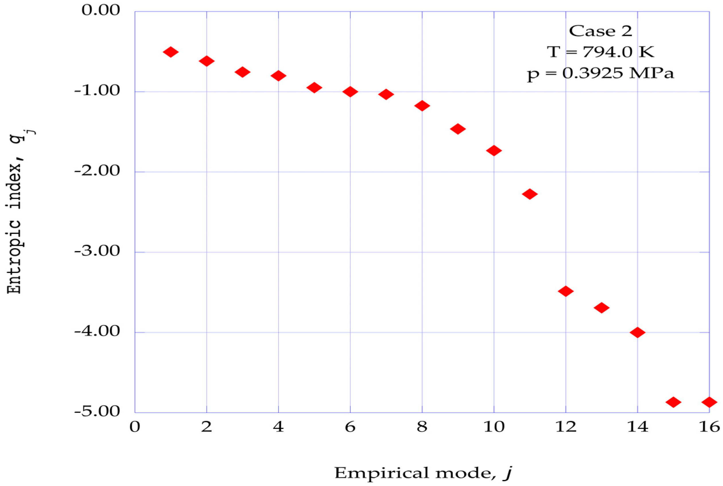
dt < 0. The results presented in Figure 8 indicate that significant non-equilibrium regions exist within the specified time frame of the particular nonlinear time series solution. These regions may therefore be classified as ordered, non-equilibrium regions. Therefore, the significant negative nature for the extracted empirical entropic indices at the third station at x = 0.120 is in agreement with both the Prigogine criterion and the Mariz results for the Tsallis entropic index. The ad hoc introduction of an empirical entropy index thus provides a representation of the nonlinear, non-equilibrium ordered regions in a significant way.
Given the absolute value of the empirical entropic index, qj, the intermittency exponent, ζj for the mode, j, is extracted from Equation (38) [22] by the use of Brent’s method [18].
Figure 9, Figure 10, Figure 11, Figure 12 and Figure 13 show the entropy generation rate at the stream wise station x = 0.120, for a normalized boundary layer distance of η = 3.00 [1] for each of the cases listed in Table 1.
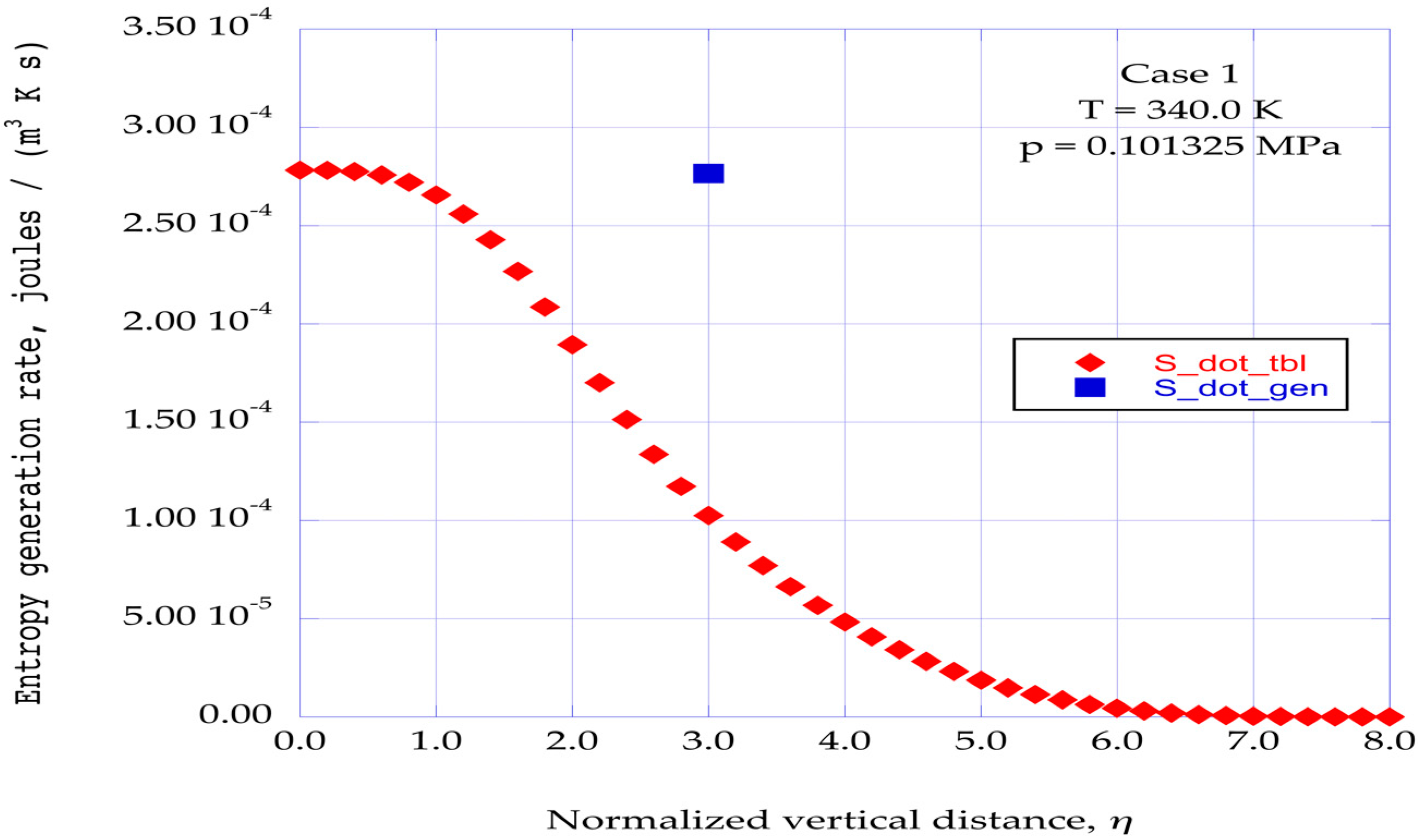
For a comparison of these values for the entropy generation rates, the entropy generation rates within a turbulent boundary layer are computed for each given stream wise location. Moore and Moore [32] give the entropy generation rate near the wall in a turbulent boundary layer as:
S t b l = τ w ρ T e ( u y ) w
Introducing the skin friction coefficient as:
C f = τ w ρ u e 2 2 ,
and applying the Falkner–Skan transformation (Equation (5)) to the velocity gradient, we may write:
S t b l = ρ ( 1 2 u e 2 T ) ( C f ) ( u e x ) ( Re x ) 1 2 ( f ) .
The often-quoted expression for the skin friction coefficient for a turbulent boundary layer on a flat plate may be written as [33]:
C f = 0.0592 ( Re x ) 1 / 5 ,
Substituting this expression for the skin friction coefficient into Equation (43) yields:
S t b l = ρ ( 1 2 u e 2 T e ) ( u e x ) ( 0.0592 ( Re x ) 0.30 ) ( f ) .
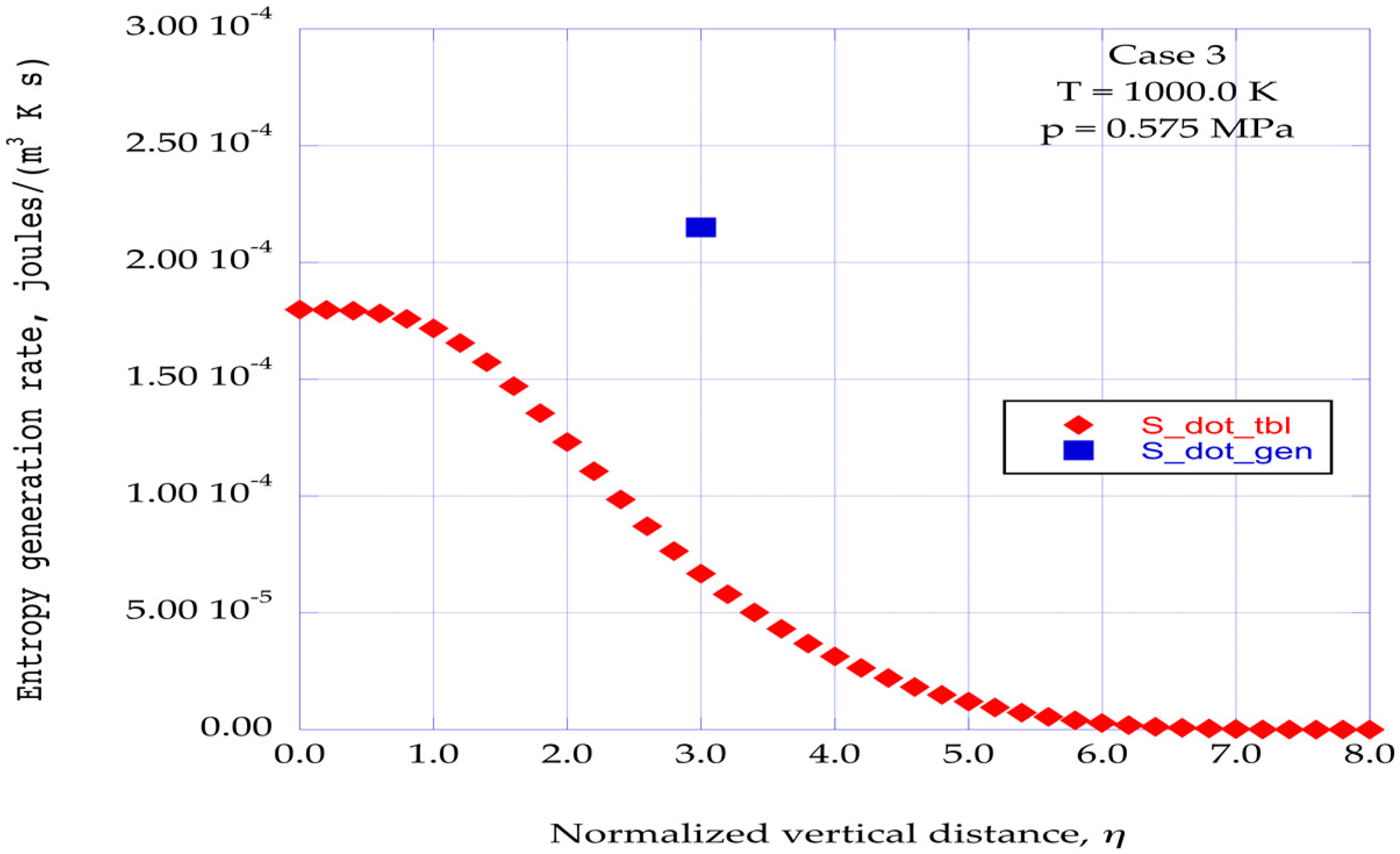
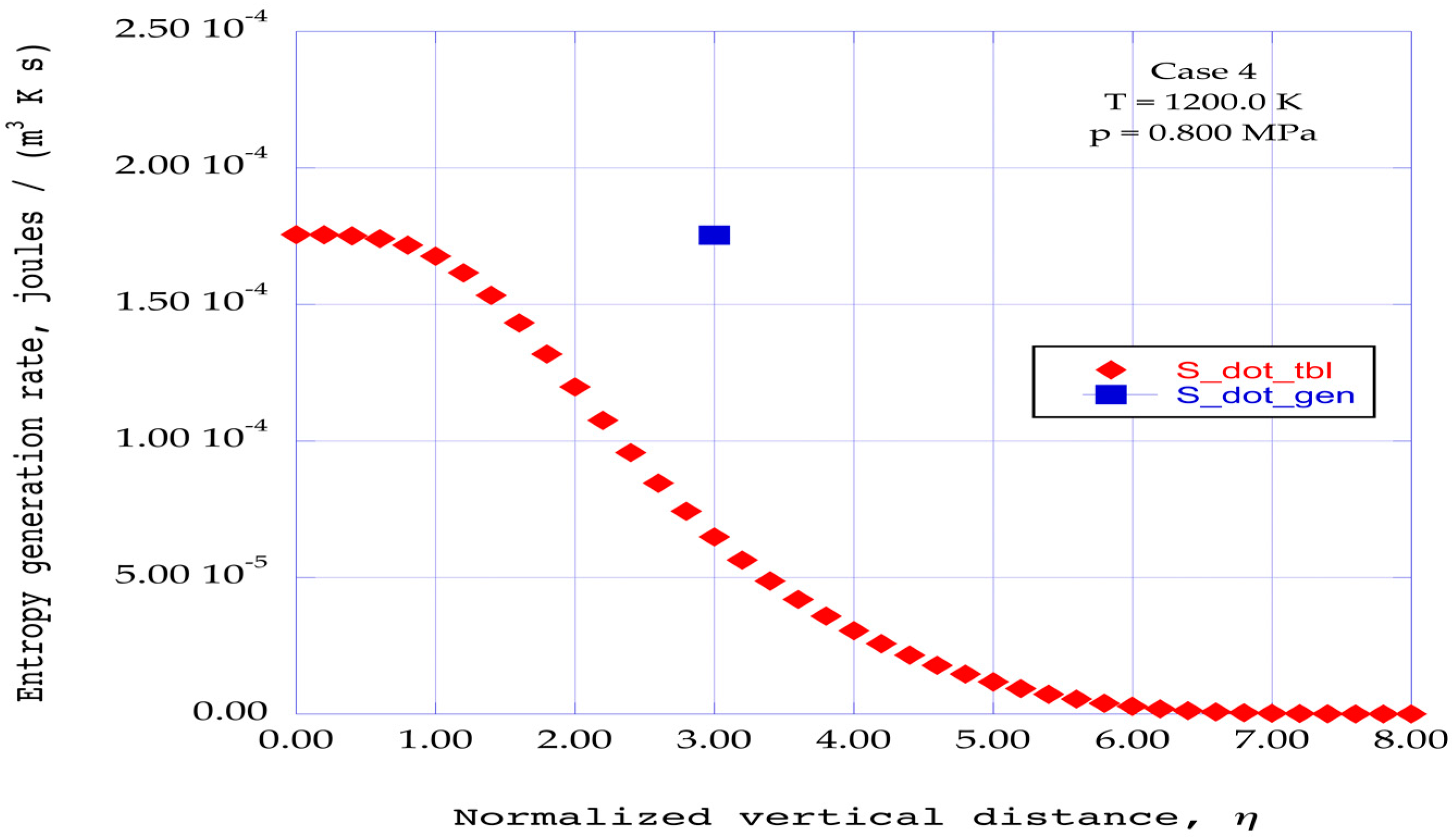
This expression is used to compute the entropy generation rates across a hypothetical turbulent boundary layer as a function of the normalized vertical distance η along the horizontal surface of the turbulent spot. The computation of the turbulent boundary layer begins at the initial station x = 0.02 with transition enforced at this location. Hence, the turbulent boundary layer for our calculations at the stream wise location x = 0.120 is much smaller than for a naturally occurring transition further along the 
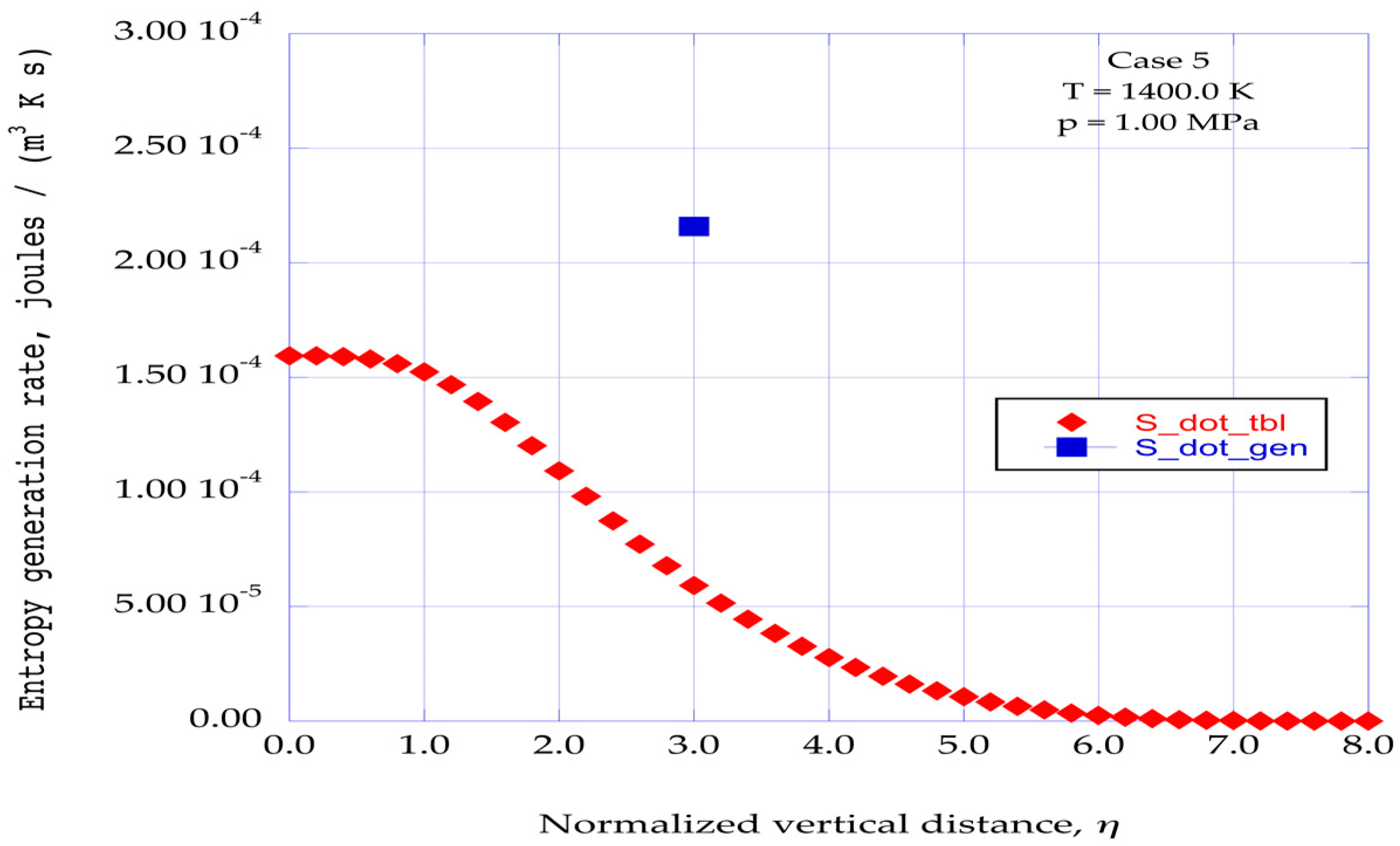
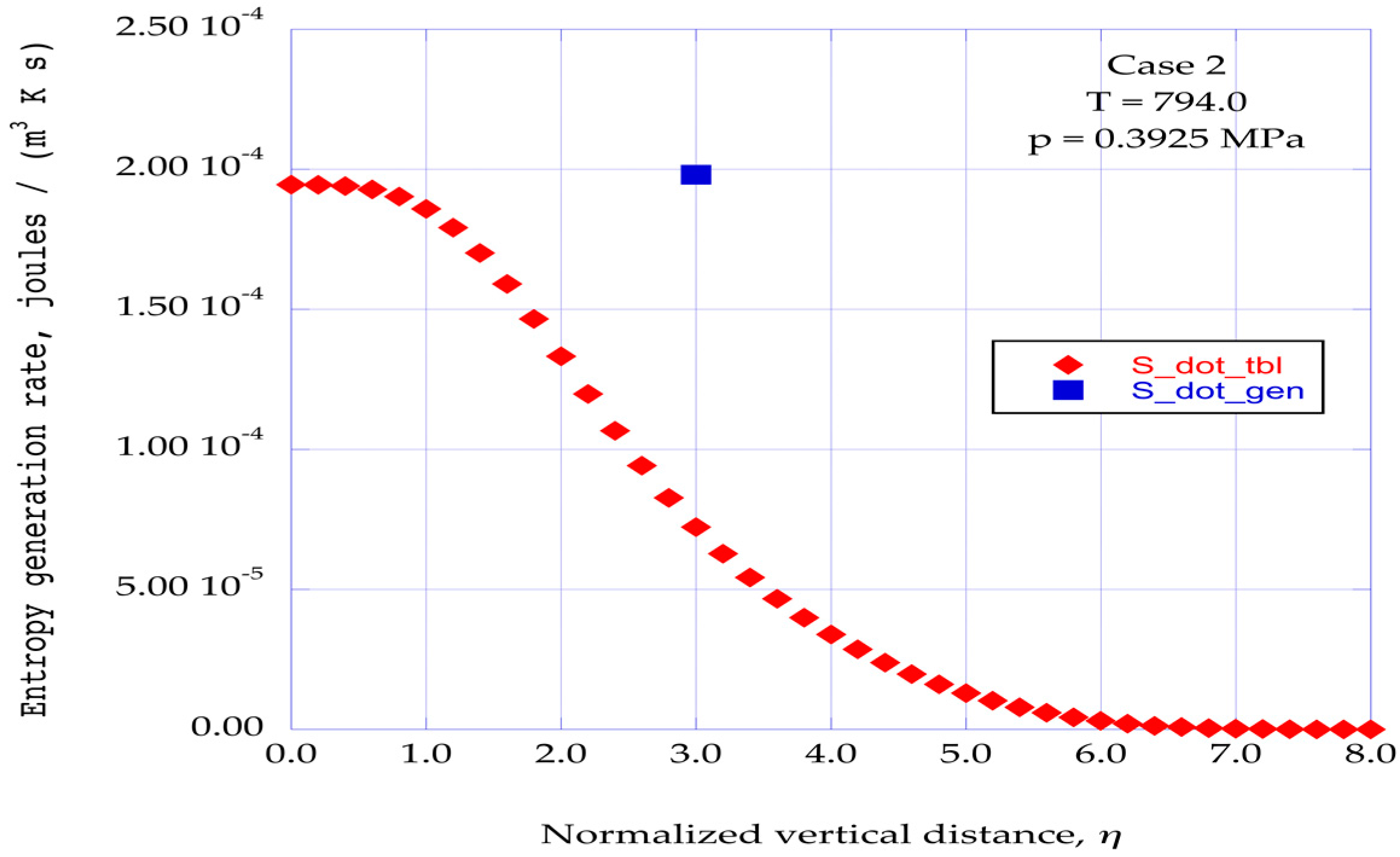
x-direction. The distributions of the entropy generation rates across a flat plate turbulent boundary layer are also shown in Figure 9, Figure 10, Figure 11, Figure 12 and Figure 13.
The contrast in the fundamental meaning of entropy generation rates between the two sets of data shown in these figure should be clarified. The entropy generation rates computed for the turbulent boundary layer use a well-established empirical relation for the turbulent skin friction coefficient (Equation (44)) and an empirical eddy viscosity expression for the computation of the mean turbulent velocity profiles across the boundary layer. These types of results are useful to the designer of thermal power equipment for the estimation of the loss in stagnation pressure due to turbulent irreversible boundary-layer processes within the system.
On the other hand, the computation of the entropy generation rates for the ordered regions (Equation (40)) proceeds from the identification of time-dependent instabilities within the laminar boundary layer due to nonlinear interactions with a vortex tangential velocity, through to the evaluation of the dissipation of energy within non-equilibrium ordered regions.
White [33] has discussed the development of turbulent spots in the stream wise transition of the flow from the initial laminar state to the fully turbulent state. Belotserkovskii and Khlopkov [7] discuss the application of Monte Carlo computational methods to predict the spread of these turbulent spots across the channel into fully turbulent flow. These methods should be applicable for the extension of the results addressed in this article to the fully developed turbulent flow region.

7. Discussion

A computational procedure made up of a steady state thermodynamic reservoir of three-dimensional boundary layer velocity gradients and an embedded time-dependent thermodynamic subsystem of coupled, nonlinear, modified Lorenz equations in the spectral plane has been applied to several helium boundary layer flows. The helium flow configuration considered is that of a turbulent spot, consisting of a counterclockwise vortex structure interacting with a stream wise laminar boundary layer profile. Computational results for entropy generation rates are presented for several different sets of temperature and pressure applicable to the flow of helium in the Helium Brayton Cycle with Interstage Heating and Cooling. This power cycle is a part of the development of Generation IV Nuclear Energy Systems.
The counter clockwise rotating stream wise vortex structure creates a viscous boundary layer along the z–y plane of the flow configuration. This viscous boundary layer is orthogonal to the laminar boundary layer in the x–y plane in the stream wise direction. It is shown that this nonlinear interaction creates instabilities within the three-dimensional flow configuration. These instabilities are produced over several stations in the stream wise direction of the flow. The computations indicate that the initial instabilities grow in strength in the stream wise direction, reach a maximum, and then decrease over the remaining stations. This stream wise structure of the region of instabilities is in close agreement with the results reported by Singer [10], obtained through the spatially developing direct numerical simulation of a young turbulent spot.
The computational results reported here for the entropy generation rates for several helium boundary layer flows are obtained at the stream wise location where the intensity of the predicted instabilities is most intense, namely, x = 0.120, in the range of instability locations from x = 0.06 to x = 0.18, for the normalized vertical station of η = 3.00.
Fluctuating spectral velocity components are found within the three spectral velocity component time-series solutions for the modified Lorenz equations. Statistical processing of the solutions indicates the presence of ordered regions embedded within the nonlinear time-series solutions. The dissipation of these ordered regions into equilibrium thermodynamic states yields the entropy generation rates for the helium turbulent spot environment. Significant entropy generation rates are predicted for the specified helium flow environments.
The sensitivity to initial conditions of the Lorenz format spectral velocity equations may provide a means of connecting the incorporation of these time dependent spectral equations in the computational procedure with the concept of receptivity of the boundary layer flow to outside disturbances.
To gain a perspective on the magnitude of the predicted rates of entropy generation through the transition of ordered regions, a comparison is made with the rates of entropy generation in a flat plate turbulent boundary layer for the same given flow conditions. The distribution of the entropy generation rates across a turbulent boundary layer at the distance of x = 0.120 is computed for a turbulent boundary layer initiated at x = 0.02 from the leading edge of the horizontal surface. The entropy generation rates through the ordered regions at the normalized vertical distance of η = 3.0 are then compared with the turbulent boundary layer distributions for each of the given helium flow conditions.
White [33] and Schlichting [34] have discussed the development of turbulent spots in the stream wise transition of the flow from the initial laminar state to the fully turbulent state. Belotserkovskii and Khlopkov [7] discuss the application of Monte Carlo simulation methods to predict the spread of turbulent spots across the channel into fully turbulent flow. The dynamic growth of the turbulent spots has been included in these simulation methods. These simulation methods appear to provide computational methods for the inclusion of the local entropy generation rates within the turbulent spots and thus evaluate the overall entropy generation rates for the fully develop turbulent flow. These methods should thus be applicable for the extension of the results presented in this article to the computational fluid dynamics of fully developed turbulent flow.

8. Conclusions

Computation of the interaction of a vortex tangential velocity with the stream wise laminar boundary layer in a helium boundary layer turbulent spot indicates the generation of non-equilibrium ordered regions within the time dependent series solutions for the three-dimensional spectral velocity components. The entropy generation rates through the dissipation of these ordered regions are computed for five sets of temperature and pressure for helium boundary layer flows. Comparison of the entropy generation rates through the dissipation of these ordered regions with the entropy generation rates in simulated turbulent boundary layers indicates that the ordered region dissipation rates are quite strong. The inclusion of time-dependent non-equilibrium spectral equations into a reservoir of steady laminar boundary layer velocity profiles may provide additional insight into the transition of laminar to turbulent flow. The application of Monte Carlo methods should allow the prediction of the spread of turbulent spots across a channel into fully developed turbulent flow, thus providing a computational path to the prediction of entropy generation rates throughout the turbulent flow.

Acknowledgments

The author would like to acknowledge the contributions of the reviewers of the manuscript for this article. A number of their observations and suggestions have been included in the article and have improved the presentation of the subject. These contributions are appreciated.

Conflicts of Interest

The author declares no conflict of interest.

Nomenclature

aiFluctuating i-th component of velocity wave vector
bFluctuating Fourier component of the static pressure
bnCoefficient in modified Lorenz equations defined by Equation (35)
CfSkin-friction coefficient
FTime-dependent feedback factor
hIntegration time step (s)
jMode number empirical eigenvalue
JNet source of kinetic energy dissipation rate, Equation (39)
kTime-dependent wave number magnitude
kiFluctuating i-th wave number of Fourier expansion
KAdjustable weighting factor
mPressure gradient parameter, Equation (11)
pLocal static pressure (N·m−2)
qjEmpirical entropic index for the empirical entropy of mode, j
rnCoefficient in modified Lorenz equations defined by Equation (33)
sEntropy per unit mass (J·kg1·K−1))
snCoefficient in modified Lorenz equations defined by Equation (34)
SempjEmpirical entropy for empirical mode, j
S g e n Entropy generation rate through kinetic energy dissipation (J·m−3·K−1·s−1)
S t b l Entropy generation rate in a turbulent boundary layer (J·m−3·K−1·s−1)
tTime (s)
uMean stream wise velocity in the x-direction in Equation (4)
uFluctuating stream wise velocity in Equation (4)
ueStream wise velocity at the outer edge of the xy plane boundary layer
uiThe i-th component of the fluctuating velocity
UiMean velocity in the i-th direction in the modified Lorenz equations
vMean normal velocity in Equation (4)
vFluctuating normal velocity in Equation (4)
weSpan wise velocity at the outer edge of the z–y plane boundary layer
xStream wise distance
xii-th direction
xjj-th direction
yNormal distance
zSpan wise distance
Greek Letters
δBoundary layer thickness (m)
δlmKronecker delta
εmEddy viscosity (m2·s−1)
ζjIntermittency exponent for the j-th mode in Equation (38)
ηTransformed normal distance parameter
κxFraction of kinetic energy in the stream wise component
κyFraction of kinetic energy in the normal component
κzFraction of kinetic energy in the span wise component
λjEigenvalue for the empirical mode, j
μMechanical potential in Equation (39)
νKinematic viscosity of the gas mixture (m2·s−1)
ξjKinetic energy in the j-th empirical mode
ρDensity (kg·m−3)
σyCoefficient in modified Lorenz equations defined by Equation (31)
σxCoefficient in modified Lorenz equations defined by Equation (32)
τwWall shear stress (N·m−2)
Subscripts
eOuter edge of the laminar boundary layer
i, j, l, mTensor indices
xComponent in the x-direction
yComponent in the y-direction
zComponent in the z-direction

References

  1. Isaacson, L.K. Entropy Generation through Deterministic Spiral Structures in Corner Flows with Sidewall Surface Mass Injection. Entropy 2016, 18, 47. [Google Scholar] [CrossRef]
  2. Isaacson, L.K. Entropy Generation through Non-equilibrium Ordered Structures in Corner Flows with Sidewall Mass Injection. Entropy 2016, 18, 279. [Google Scholar] [CrossRef]
  3. Walsh, E.J.; Hernon, E. Unsteady Volumetric Entropy Generation Rate in Laminar Boundary Layers. Entropy 2006, 8, 25–30. [Google Scholar] [CrossRef]
  4. Boiko, A.V.; Grek, G.R.; Dovgal, A.V.; Kozlov, V.V. The Origin of Turbulence in Near-Wall Flows; Springer: Berlin, Germany, 2010; pp. 115–119. [Google Scholar]
  5. Wright, S.A.; Vernon, M.E.; Pickard, P.S. Concept Design for a High Temperature Helium Brayton Cycle with Interstage Heating and Cooling; Sandia Report SAND2006-4147; Sandia National Laboratories: Albuquerque, NM, USA, 2006. [Google Scholar]
  6. Schmid, P.J.; Henningson, D.S. Stability and Transition in Shear Flows; Springer: New York, NY, USA, 2001; pp. 401–465. [Google Scholar]
  7. Belotserkovskii, O.M.; Khlopkov, Y.I. Monte Carlo Methods in Mechanics of Fluid and Gas; World Scientific Publishing: Singapore, 2010. [Google Scholar]
  8. Townsend, A.A. The Structure of Turbulent Shear Flow, 2nd ed.; Cambridge University Press: Cambridge, UK, 1976. [Google Scholar]
  9. Hellberg, C.S.; Orszag, S.A. Chaotic behavior of interacting elliptical instability modes. Phys. Fluids 1988, 31, 6–8. [Google Scholar] [CrossRef]
  10. Singer, B.A. Characteristics of a young turbulent spot. Phys. Fluids 1996, 8, 509–521. [Google Scholar] [CrossRef]
  11. Ersoy, S.; Walker, J.D.A. Viscous flow induced by counter-rotating vortices. Phys. Fluids 1985, 28, 2687–2698. [Google Scholar] [CrossRef]
  12. Cebeci, T.; Bradshaw, P. Momentum Transfer in Boundary Layers; Hemisphere: Washington, DC, USA, 1977; pp. 319–321. [Google Scholar]
  13. Cebeci, T.; Cousteix, J. Modeling and Computation of Boundary-Layer Flows; Horizons Publishing: Long Beach, CA, USA, 2005. [Google Scholar]
  14. Hansen, A.G. Similarity Analyses of Boundary Value Problems in Engineering; Prentice-Hall: Englewood Cliffs, NJ, USA, 1964; pp. 86–92. [Google Scholar]
  15. Isaacson, L.K. Control Parameters for Boundary-Layer Instabilities in Unsteady Shock Interactions. Entropy 2012, 14, 131–160. [Google Scholar] [CrossRef]
  16. Attard, P. Non-Equilibrium Thermodynamics and Statistical Mechanics: Foundation and Applications; Oxford University Press: Oxford, UK, 2012. [Google Scholar]
  17. Sparrow, C. The Lorenz Equations: Bifurcations, Chaos, and Strange Attractors; Springer: New York, NY, USA, 1982. [Google Scholar]
  18. Mathieu, J.; Scott, J. An Introduction to Turbulent Flow; Cambridge University Press: New York, NY, USA, 2000; pp. 251–261. [Google Scholar]
  19. Press, W.H.; Teukolsky, S.A.; Vetterling, W.T.; Flannery, B.P. Numerical Recipes in C: The Art of Scientific Computing, 2nd ed.; Cambridge University Press: Cambridge, UK, 1992. [Google Scholar]
  20. Manneville, P. Non-Equilibrium Regions and Weak Turbulence; Academic Press: San Diego, CA, USA, 1990. [Google Scholar]
  21. Pecora, L.M.; Carroll, T.L. Synchronization in chaotic systems. Phys. Rev. Lett. 1990, 64, 821. [Google Scholar] [CrossRef] [PubMed]
  22. Pérez, G.; Cerdeiral, H.A. Extracting messages masked by chaos. Phys. Rev. Lett. 1995, 74, 1970. [Google Scholar] [CrossRef] [PubMed]
  23. Cuomo, K.M.; Oppenheim, A.V. Circuit implementation of synchronized chaos with applications to communications. Phys. Rev. Lett. 1993, 71, 65. [Google Scholar] [CrossRef] [PubMed]
  24. Chen, C.H. Digital Waveform Processing and Recognition; CRC Press: Boca Raton, FL, USA, 1982; pp. 131–158. [Google Scholar]
  25. Holmes, P.; Lumley, J.L.; Berkooz, G.; Rowley, C.W. Turbulence, Coherent Structures, Dynamical Systems and Symmetry, 2nd ed.; Cambridge University Press: Cambridge, UK, 2012. [Google Scholar]
  26. Rissanen, J. Information and Complexity in Statistical Modeling; Springer: New York, NY, USA, 2007. [Google Scholar]
  27. Tsallis, C. Introduction to Nonextensive Statistical Mechanics; Springer: New York, NY, USA, 2009; pp. 37–43. [Google Scholar]
  28. Arimitsu, T.; Arimitsu, N. Analysis of fully developed turbulence in terms of Tsallis statistics. Phys. Rev. E 2000, 61, 3237–3240. [Google Scholar] [CrossRef]
  29. De Groot, S.R.; Mazur, P. Non-Equilibrium Thermodynamics; North-Holland Pub. Co.: Amsterdam, The Netherlands, 1962. [Google Scholar]
  30. Glansdorff, P.; Prigogine, I. Thermodynamic Theory of Structure, Stability and Fluctuations; Wiley: London, UK, 1971. [Google Scholar]
  31. Mariz, A.M. On the irreversible nature of the Tsallis and Renyi entropies. Phys. Lett. A 1992, 165, 409–411. [Google Scholar] [CrossRef]
  32. Moore, J.; Moore, J.G. Entropy Production Rates from Viscous Flow Calculations: Part I—A Turbulent Boundary Layer Flow. In Proceedings of the 28th International Gas Turbine Conference and Exhibit, Phoenix, AZ, USA, 27–31 March 1983. [Google Scholar]
  33. White, F.M. Viscous Fluid Flow; McGraw-Hill: New York, NY, USA, 1974. [Google Scholar]
  34. Schlichting, H. Boundary-Layer Theory; McGraw-Hill Book Company: New York, NY, USA, 1979. [Google Scholar]
Figure 1. Shown in this figure is a schematic diagram of the configuration of the vortex tangential velocity boundary layer profile in the zy plane normal to the stream wise boundary layer profile in the xy plane for the left-hand side of a turbulent spot.
Entropy 19 00278 g001
Figure 2. Entropy generation computational flow chart.
Entropy 19 00278 g002
Figure 3. Shown is the stream wise deterministic trajectory of the spectral velocity component, ax3, for Case 2 at x = 0.120 for η = 3.0 and we = 0.080.
Entropy 19 00278 g003
Figure 4. Shown is a graph of the normal spectral velocity component, ay3, versus the stream wise spectral velocity component, ax3, for Case 2 at x = 0.120, η = 3.00 and we = 0.080.
Entropy 19 00278 g004
Figure 5. The phase diagram of the span wise and normal spectral velocity components, az3ay3, for Case 2, is shown for x = 0.120, η = 3.00 and we = 0.080.
Entropy 19 00278 g005
Figure 6. A three-dimensional representation of the deterministic trajectories of the spectral velocity components, ax3, ay3, and az3, for Case 2, is shown for x = 0.120, η = 3.00 and we = 0.080.
Entropy 19 00278 g006
Figure 7. The power spectral density for the normal spectral velocity component, ay3, for Case 2, is shown for x = 0.120, η = 3.00 and we = 0.080.
Entropy 19 00278 g007
Figure 8. The entropic index, q, as a function of the empirical mode, j, for the span wise spectral velocity component ay3, is shown for Case 2, at x = 0.120, η = 3.00 and we = 0.080.
Entropy 19 00278 g008
Figure 9. The entropy generation rate for the helium boundary layer for Case 1 at a temperature of 340.0 K and a pressure of 0.101325 MPa at the stream wise location of x = 0.120, η = 3.00 and we = 0.080. Also shown is the entropy generation rate distribution across a turbulent boundary layer at the stream wise location of x = 0.120. The turbulent boundary layer is artificially generated at x = 0.020.
Entropy 19 00278 g009
Figure 10. The entropy generation rate for the helium boundary layer at a temperature of 794.0 K and a pressure of 0.3925 MPa at the stream wise location of x = 0.120, η = 3.00 and we = 0.080. Also shown is the entropy generation rate distribution across a turbulent boundary layer at the stream wise location of x = 0.120.
Entropy 19 00278 g010
Figure 11. The entropy generation rate for the helium boundary layer for Case 3 at the stream wise location of x = 0.120, η = 3.00 and we = 0.080. Also shown is the entropy generation rate distribution across a turbulent boundary layer at the stream wise location of x = 0.120.
Entropy 19 00278 g011
Figure 12. The entropy generation rate for the helium boundary layer for Case 4 at the stream wise location of x = 0.120, η = 3.00 and we = 0.080. Also shown is the entropy generation rate distribution across a turbulent boundary layer at the stream wise location of x = 0.120.
Entropy 19 00278 g012
Figure 13. The entropy generation rate for the helium boundary layer for Case 5 at the stream wise location of x = 0.120, η = 3.00 and we = 0.080. Also shown is the entropy generation rate distribution across a turbulent boundary layer at the stream wise location of x = 0.120.
Entropy 19 00278 g013
Table 1. This table provides the temperature and pressure, with the corresponding kinematic viscosity, for each of the cases considered.
Case NumberTemperature, T (K)Pressure, p (MPa)Kinematic Viscosity, v (m2/s)
1340.00.1013251.530133 × 10−4
2794.00.39251.597516 × 10−4
31000.00.57501.594692 × 10−4
41200.00.80001.547814 × 10−4
51400.01.00001.596312 × 10−4

