Article

Time-Shift Multiscale Entropy Analysis of Physiological Signals

Department of Biomedical Engineering, Linköping University, 581 83 Linköping, Sweden
Entropy 2017, 19(6), 257; https://doi.org/10.3390/e19060257
Submission received: 17 April 2017 / Revised: 1 June 2017 / Accepted: 2 June 2017 / Published: 5 June 2017
(This article belongs to the Special Issue Entropy in Signal Analysis)

Abstract

:
Measures of predictability in physiological signals using entropy measures have been widely applied in many areas of research. Multiscale entropy expresses different levels of either approximate entropy or sample entropy by means of multiple factors for generating multiple time series, enabling the capture of more useful information than using a scalar value produced by the two entropy methods. This paper presents the use of different time shifts on various intervals of time series to discover different entropy patterns of the time series. Examples and experimental results using white noise, 1 / f noise, photoplethysmography, and electromyography signals suggest the validity and better performance of the proposed time-shift multiscale entropy analysis of physiological signals than the multiscale entropy.

1. Introduction

The notion of the approximate entropy (ApEn) [1], which quantifies irregularity or predictability in scalar time series has been increasingly applied in various scientific domains of signal processing. The modified version of ApEn known as the sample entropy (SampEn) [2] was introduced to remove self-matching in ApEn, and reported to produce results better than the use of ApEn in several studies of time-series analysis [3,4,5].
Consider a scalar time series X of length N taken at regular intervals: X = ( x 1 , x 2 , , x N ) , and a given embedding dimension m, a set of newly reconstructed time series from X, denoted as Y, can be established as Y = ( y 1 , y 2 , , y N - m + 1 ) , where y i = ( x i , x i + 1 , , x i + m - 1 ) , i = 1 , 2 , , N - m + 1 . Given a positive tolerance value r, the probability of vector y i being similar to vector y j is computed as
C i m ( r ) = 1 N - m + 1 j = 1 N - m + 1 θ [ d ( y i , y j ) ] ,
where θ ( d ( y i , y j ) ) is the step function defined as
θ [ d ( y i , y j ) ] = 1 : d ( y i , y j ) r , 0 : d ( y i , y j ) > r .
The distance between the two vectors can be obtained by
d ( y i , y j ) = max k ( | x i + k - 1 - x j + k - 1 | ) , k = 1 , 2 , , m .
The probabilities of all vectors being similar to one another are computed as
C m ( r ) = 1 N - m + 1 i = 1 N - m + 1 log [ C i m ( r ) ] .
Approximate entropy, denoted as ApEn, is defined as
ApEn = C m ( r ) - C m + 1 ( r ) .
For the calculation of ApEn, m = 2 or 3, and r = 0.1 to 0.25 × σ , where σ is standard deviation of the time series, were typically suggested [6]. Let B i m ( r ) be defined as
B i m ( r ) = 1 N - m - 1 j = 1 N - m θ [ d ( y i , y j ) ] , i j .
Thus, B m ( r ) is given by
B m ( r ) = 1 N - m i = 1 N - m B i m ( r ) .
The formulation of SampEn is expressed as
SampEn = - log B m + 1 ( r ) B m ( r ) .
In particular, the multiscale entropy (MSE) [7] was developed to measure entropy such as SampEn at different scales by averaging non-overlapping time points of the original time series in order to better reveal patterns of predictability or regularity in the time series. The use of MSE analysis of time series is able to explain the inconsistency encountered with single-scale analysis in the increase and decrease in entropy values of certain physiological signals, and have been found useful in many applications, most recently such as [8,9,10,11]. The MSE works by applying a “coarse-graining” process to the original time series to generate several time series of different scales, and then computing either SampEn or ApEn for all coarse-grained time series, which are plotted as a function of the scale factor. Consider the time series X of length N taken at regular intervals: X = ( x 1 , x 2 , , x N ) . For a scale factor τ , a new time series X τ is created by the MSE as follows [7]:
X j τ = 1 τ i = ( j - 1 ) τ + 1 j τ x i , 1 j N / τ .

2. Time-Shift Multiscale Entropy

The proposed time-shift multiscale entropy, denoted as TSME, is motivated by a popular approach for computing the fractal dimension of irregular time series, known as the Higuchi’s fractal dimension (HFD) [12]. The HFD computes the “mean length" of the curve of a time series by constructing a set of new time series that has the property of a fractal curve over all time scales as each time series can be considered a reduced scale form of the whole. A set of new time series constructed from the original time series by the HFD, which are utilized in this study, are based on the consideration of the phase distribution. This phase distribution can reveal strong effects of the irregularity of time series [13]. In fact, it has been reported that the HFD is a stable numerical approach for time series analysis, including stationary, nonstationary, deterministic, and stochastic signals [14,15,16,17]. Therefore, the time-shift multiscale entropy can be expected to be applied to these types of signals for studying irregularity in time series.
The new time series generated by the HFD are constructed as follows by once again considering the time series X of length N : X = ( x 1 , x 2 , , x N ) . Let β and k be positive integers, where β = 1 , 2 , , k , then k new time series can be generated using the following equation [12]:
X k β = ( x β , x β + k , x β + 2 k , , x β + N - β k k ) ,
where N - β k is the “floor” function that rounds N - β k to the largest integer not exceeding N - β k .
From Equation (10), β and k indicate the initial time point and time interval, respectively, that is, for a given time interval k, k new time series are constructed using k time shifts. For example [18], let k = 3, and N = 100, three new time series are generated as: X k = 3 β = 1 : ( x 1 , x 4 , x 7 , , x 100 ) , X k = 3 β = 2 : ( x 2 , x 5 , x 8 , , x 98 ) , and X k = 3 β = 3 : ( x 3 , x 6 , x 9 , , x 99 ) .
The proposed TSME method works by constructing k time-shift series for a given time interval k, then computing either SampEn or ApEn for all time-shift time series, denoted as T S M E k β , β = 1, ..., k. The TSME for each k, denoted as T S M E k , k = 1, ..., k m a x , is defined as the average value of all T S M E k β , that is,
T S M E k = 1 k β = 1 k T S M E k β .
The procedure for computing TSME is described as follows:
  • Given a scalar time series X, dimension m, tolerance r, and k m a x .
  • Set k = 1.
  • Using Equation (10) to construct k time-shift time series from X : X k β , β = 1 , , k .
  • For each X k β , β = 1 , , k , compute T S M E k β .
  • Compute T S M E k using Equation (11).
  • Set k = k + 1 .
  • Repeat steps 3–6 until k = k m a x .

3. Results and Discussion

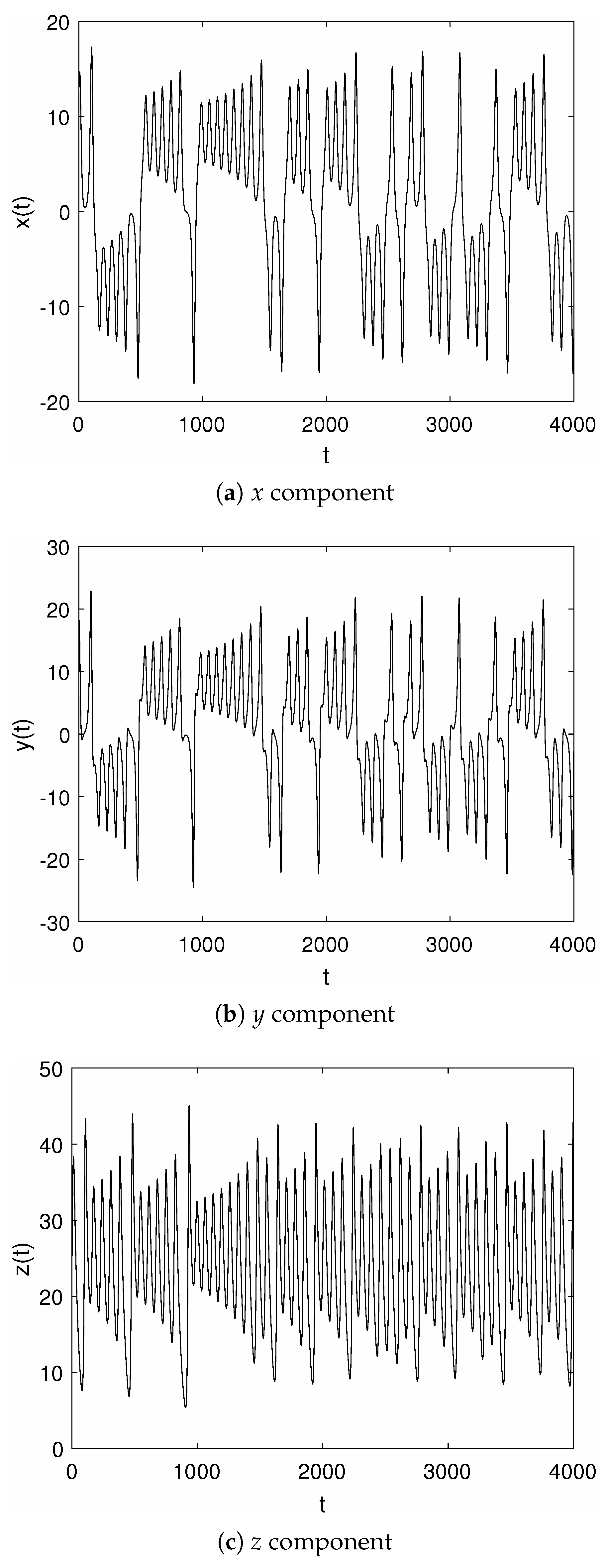
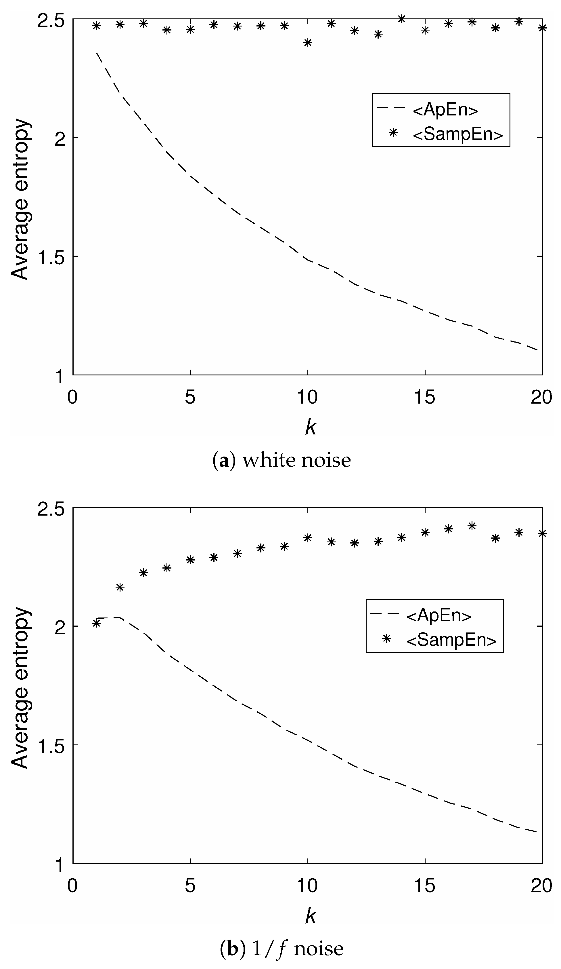
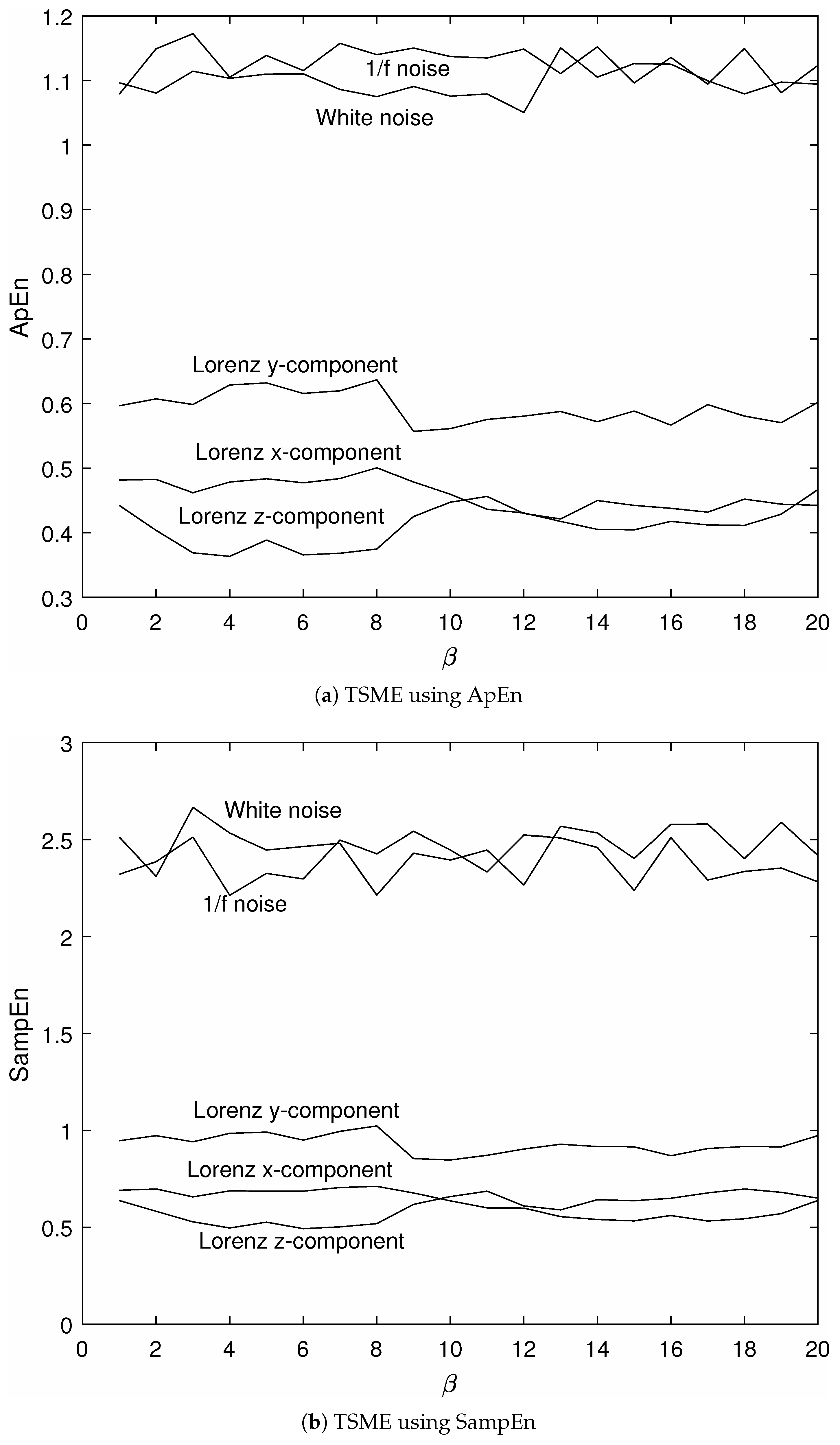
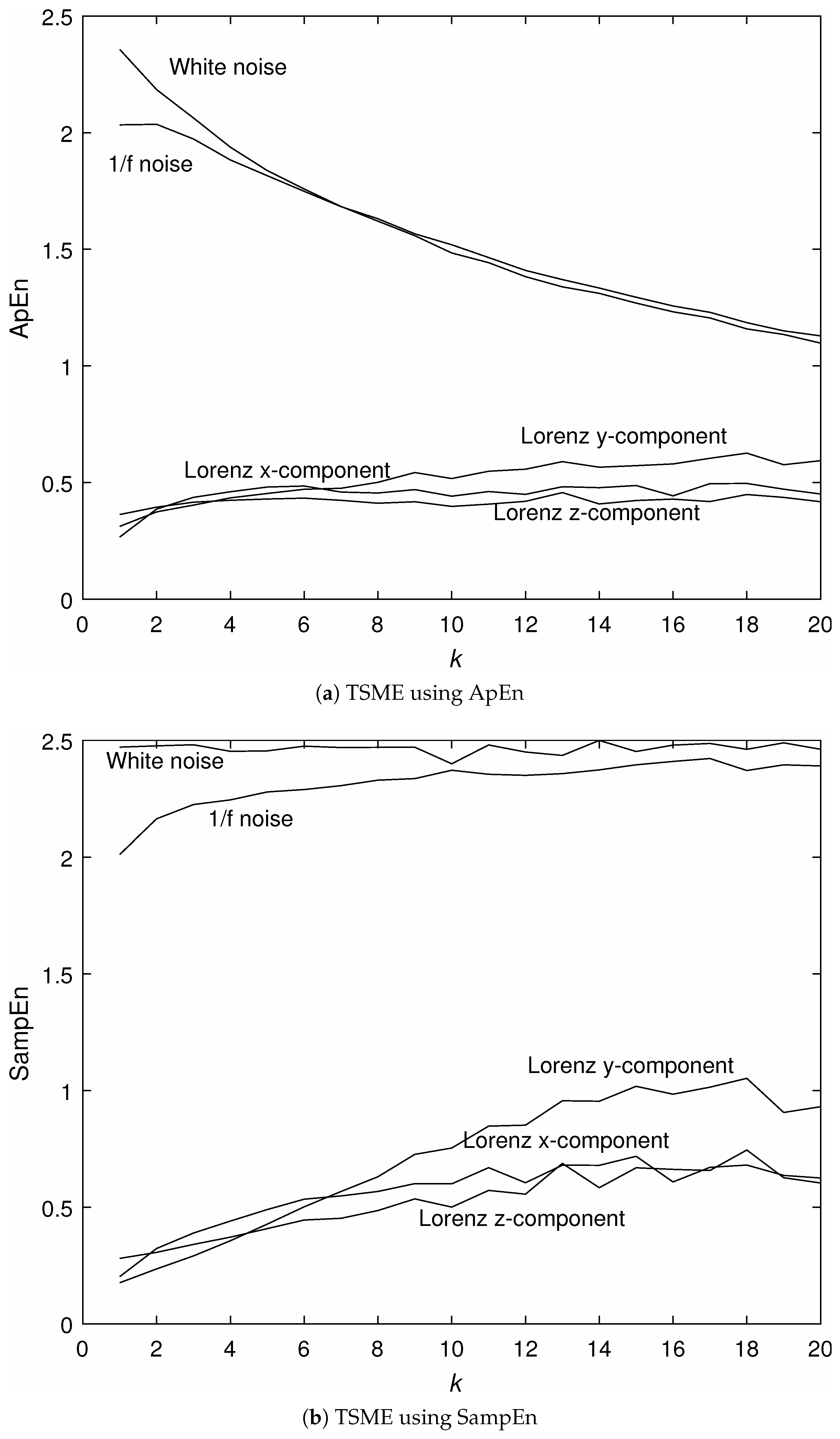
3.1. Analysis of Signals with Known Properties

In signal processing, white noise and 1 / f (pink) noise are signals with known statistical properties, which are widely found as good approximation of many real-world data and generate mathematically tractable models. Time series of white noise are sequences of serially uncorrelated random variables with zero mean and finite variance, having equal intensity at different frequencies and constant power spectral density [19]. Time series of 1 / f noise is a signal with a frequency spectrum such that the power spectral density is inversely proportional to the frequency of the signal; it is an intermediate between the white noise and random walk noise with no correlation between increments [20]. Signals of white noise (mean = 0 and variance = 1), and 1 / f noise, both consist of 10,000 samples, were used in this analysis. Another type of signal of known property is the Lorenz system [21], consisting of x (convection velocity), y (temperature difference), and z (temperature gradient) components, which are well known to be chaotic as shown in Figure 1. These three signals, each having the length of 4000 samples, behave irregularly with time: the x and y components fluctuate around positive and negative values, and the z component oscillates around the range from about 10 to 40.
To carry out the TSME analysis, we set m = 2 and r = 0 . 15 × σ , where σ is the standard deviation of the original time series, to compute ApEn and SampEn. With k m a x = 10, the ApEn-based T S M E k β tends to slightly decrease with increasing k from 2.4 for k = 1 to 1.4 for k = 10, while the SampEn-based T S M E k β remains fairly constant around the value of 2.4. Figure 2 shows the T S M E k of the white noise and 1 / f noise, respectively, where the SampEn-based T S M E k for both signals are fairly constant. Both SampEn-based T S M E k β and SampEn-based T S M E k meet the expectation for the analysis of randomly generated time series. The trend in ApEn-based T S M E k β and ApEn-based T S M E k should be due to the bias of self-matching in the computation of ApEn [2].
Figure 3 shows that T S M E k β using either ApEn or SampEn can distinguish white noise and 1 / f noise from the chaotic time series of the Lorenz system. Similarly, Figure 4 shows that T S M E k using either ApEn or SampEn can distinguish white noise and 1 / f noise from the chaotic time series. Particularly, T S M E k can also separate white noise from 1 / f noise. T S M E k β and T S M E k values of white noise and 1 / f noise are higher than those of the three chaotic time series as shown in Figure 3 and Figure 4, respectively, which suggest the reliability of the TSME analysis, as chaotic signals are deterministic and therefore more predictable than noise data.

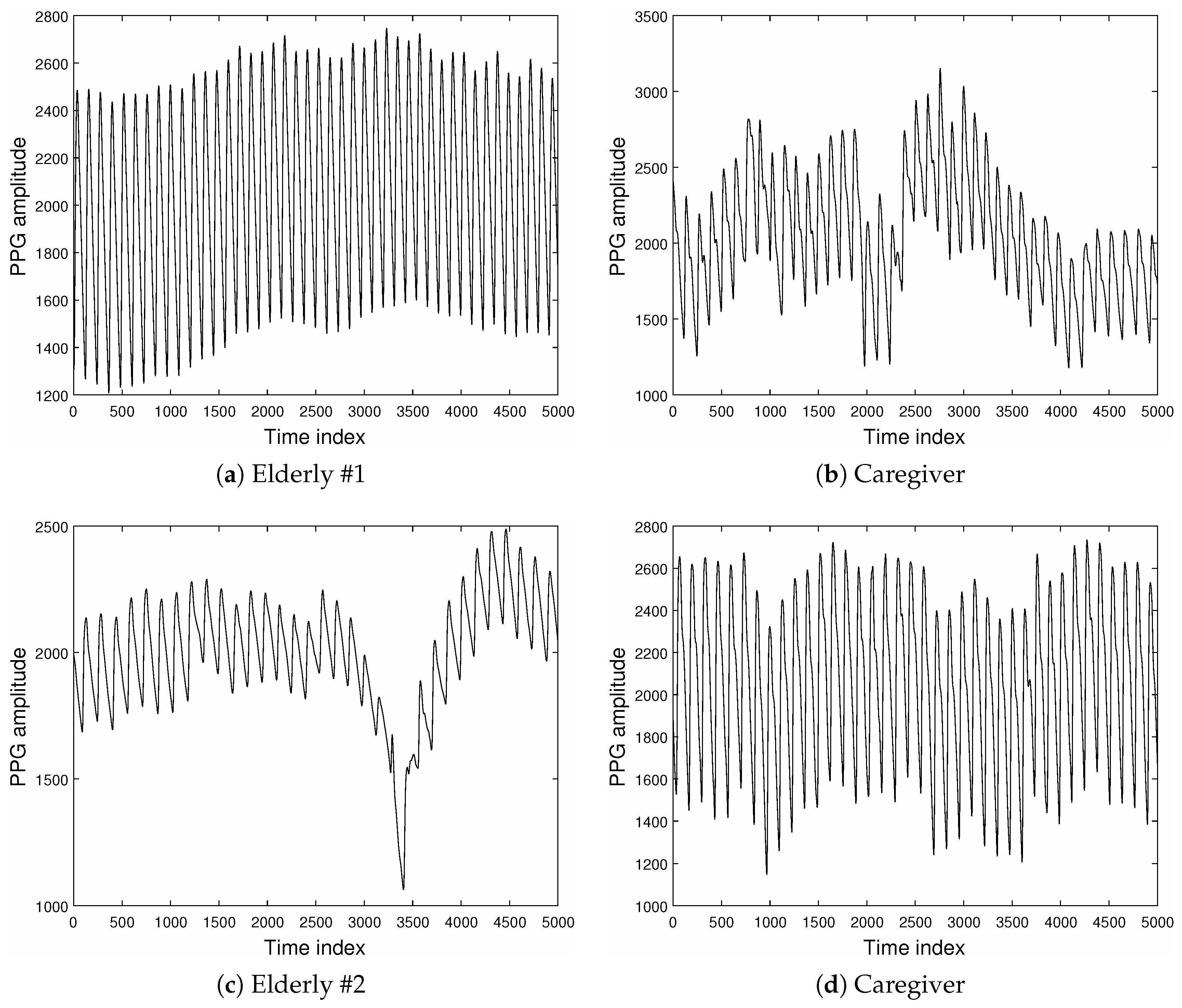
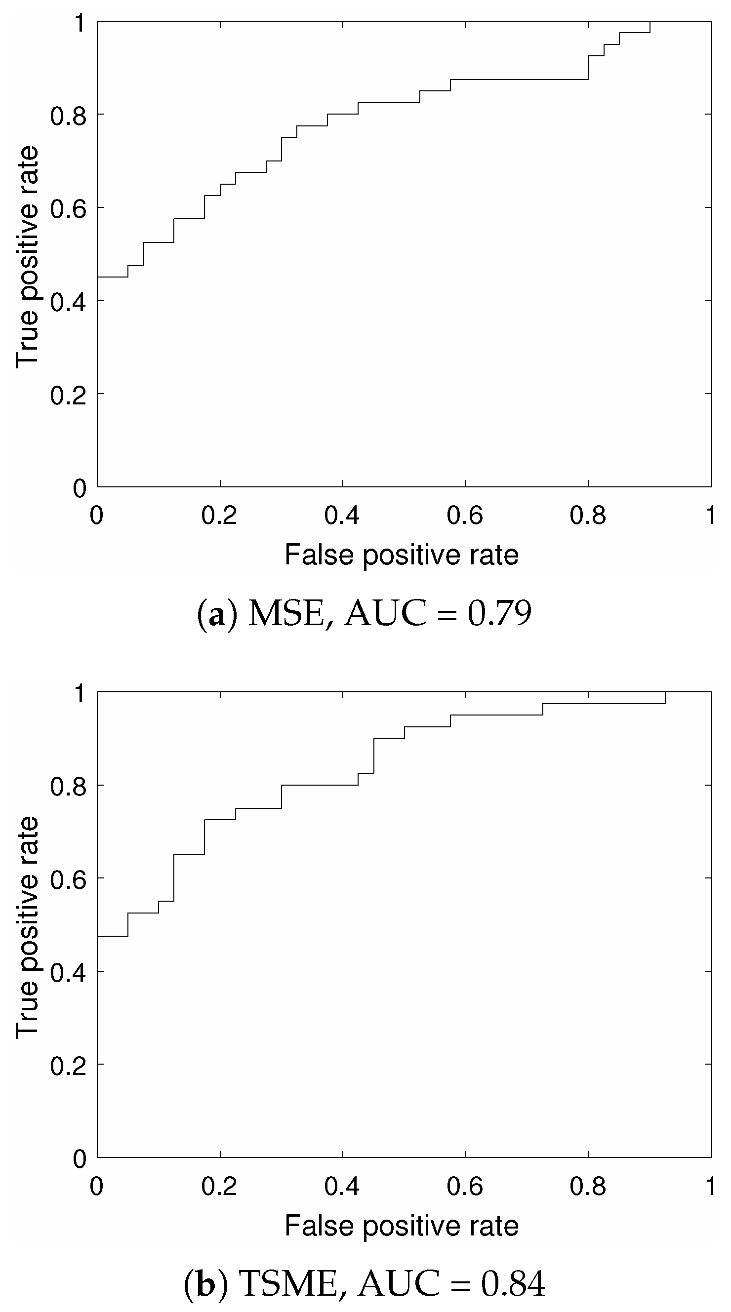
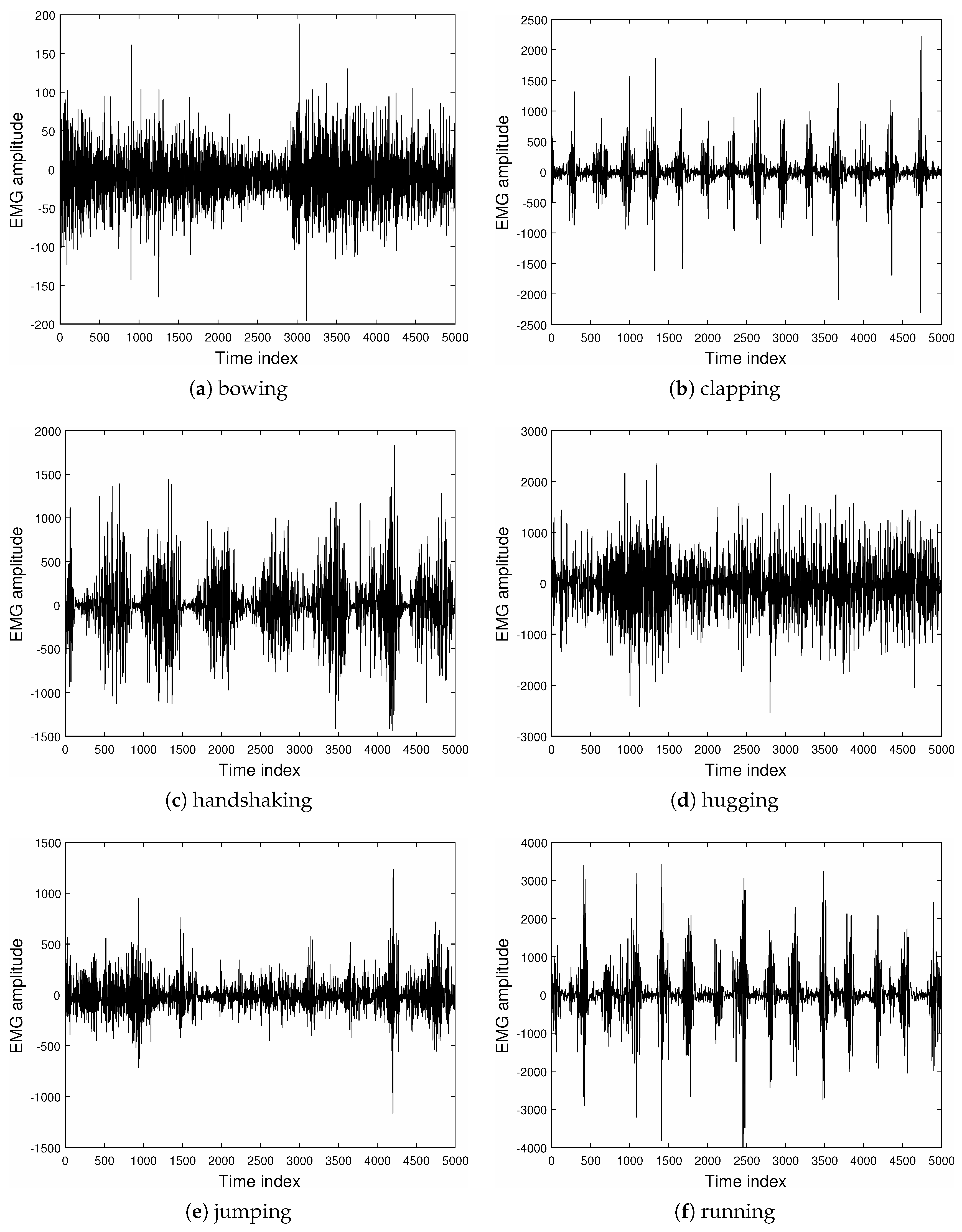
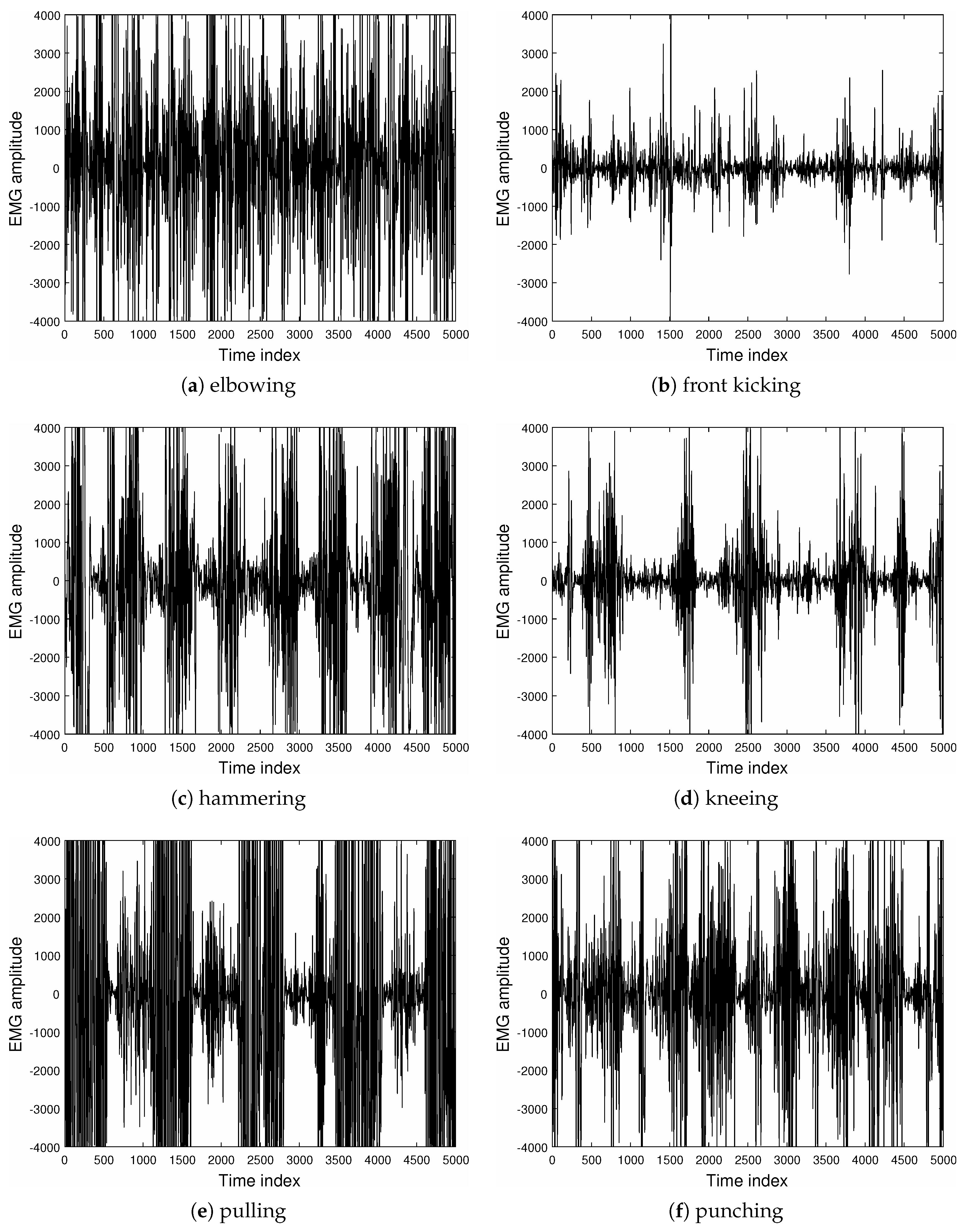
3.2. Analysis of PPG and EMG Signals

To illustrate the performance of the proposed TSME and comparison with the MSE, experiments using the photoplethysmography (PPG) and electromyography (EMG) signals are presented. The pulses of the index fingers of the left hands of 43 elderly participants and the middle-age caregiver were synchronously measured with a PPG sensor, and studied in [22] for automated assessment of therapeutic communication for cognitive stimulation for people with cognitive decline. The EMG signals were obtained from the Physical Action Data Set [23], where the channel measured on the right bicep of the participants with the Delsys EMG wireless apparatus was used in this study, for the classification of normal and aggressive human physical actions. Figure 5 shows the first 5000 samples of synchronized PPG signals of two elderly participants and the caregiver. Figure 6 shows the first 5000 samples of the EMG signals of six normal actions: bowing, clapping, handshaking, hugging, jumping, and running. Figure 7 shows the first 5000 samples of the EMG signals of six aggressive actions: elbowing, front kicking, hammering, kneeing, pulling, and punching.
For the MSE analysis, we set τ = 20 to compute X j τ expressed in Equation (9) as the MSE feature of 20 scale factors. For the TSME, we set k m a x = 20 to compute T S M E k expression in Equation (11) as the TSME feature of 20 phase shifts. Only SampEn was used in this analysis for computing both MSE and TSME, with m = 2 and r = 0 . 15 × σ , where again σ is the standard deviation of the original time series. Both PPG and EMG datasets were used for pattern classification.
The first 5000 samples of the synchronized, de-trended PPG signals of 43 elderly participants and the middle-age caregiver were used to classify the PPG signals of the elderly from the caregiver. MSE and TSME features using SampEn were extracted from these signals, and classified using the linear discriminant analysis (LDA) [24,25]. The leave-one-out (LOO) cross validation was applied to test the accuracy of LDA-based classification of the two types of features. Figure 8 shows the areas under the receiver operating characteristic (ROC) curves [26], denoted as AUC (area under curve), obtained from the MSE and TSME features extracted from the PPG signals, where the AUC of the MSE = 0.74, and the AUC of the TSME = 0.84 (the higher the value of the AUC, the better the performance). Table 1 shows the sensitivity (the rate of elderly features that are correctly identified), specificity (the rate of caregiver features that are correctly identified), and accuracy rates obtained from the LDA using the MSE and TSME features. The TSME feature yielded better results than the MSE feature in terms of accuracy and receiver operating characteristics.
The first 5000 samples of the EMG right bicep signals of the four subjects in the Physical Action Data Set [23] were also used for the differentiating normal from aggressive actions, using LDA analysis with MSE and TSME features. The experiments were carried out on each subject performing ten normal and ten aggressive physical actions that represented human activities. The ten normal actions are: (1) bowing; (2) clapping; (3) handshaking; (4) hugging; (5) jumping; (6) running; (7) seating; (8) standing; (9) walking; and (10) waving. The ten aggressive actions include: (1) elbowing; (2) front kicking; (3) hammering; (4) heading; (5) kneeing; (6) pulling; (7) punching; (8) pushing; (9) side kicking; and (10) slapping. Figure 9 shows the ROC areas under curves obtained from the MSE and TSME features, where the AUC of the MSE = 0.79, and the AUC of the TSME = 0.84, showing the better performance of the TSME. Table 2 shows the sensitivity (the rate of aggressive action features that are correctly identified), specificity (the rate of normal action features that are correctly identified), and accuracy rates obtained from the LDA using the MSE and TSME features. Once again, the TSME feature yielded better results than the MSE feature in general. The specificity (77.50%) obtained from the MSE is 5% higher than the specificity (72.50%) obtained from the TSME, while the sensitivity (67.50%) obtained from the MSE is 15% lower than the sensitivity (82.50%) obtained from the TSME, and the accuracy (50%) of the MSE is 11.25% lower than the accuracy (61.25%) of the TSME.

4. Conclusions

A method for computing SampEn or ApEn on multiple time shifts has been presented and discussed. The use of SampEn is more theoretically sound for computing TSME, as it is adopted for computing MSE. The construction of the new time series for computing the entropy profiles introduced in this study was known to be able to provide stable time scale and indices corresponding to the characteristics of irregular time series, including short time series, by taking into account self-similarity across the characteristic time scale [12]. While MSE uses the averaging of time series on several interval scales, the proposed TSME applies time shifting in time series that is based on the calculation of the “mean length” of the curve of a time series implemented in the Higuchi’s fractal dimension.
The examples using noise and chaotic time series suggest the validity of the TSME, and classification results using the physiological data illustrate the better performance of the TSME over the MSE. The computational time required for computing the TSME is higher than for computing the MSE, particularly when k m a x is large. Being similar to the specification of the τ parameter used in the MSE, an optimal selection for the k m a x used in the TSME is still an ad hoc choice reported in many studies [17], which needs further investigation. Future development of the TSME for multivariate multiscale entropy is worth pursuing, as it has been formulated based on the concept of the MSE [27,28]. An extension of the differential Shannon entropy rate of time series using kernel density estimators for selecting the order and bandwidth parameters [29] may have implications for improving the performance of the TSME.
As another issue for the implementation of the TSME regarding a good selection of the tolerance parameter r in the computation of ApEn or SampEn, the quadratic sample entropy (QSE) [30] was introduced as a complementary stochastic approach to measuring complexity by adding log ( 2 r ) to the deterministic approach ApEn or SampEn so that r can be optimally varied for individual time series. In studying neonatal heart rate data with transient decelerations, it was shown that, for the stochastic approach, the entropy tends to be converging as r approaches 0, while for the deterministic approach (SampEn), the entropy is diverging [30]. The QSE also found potential in the application to the analysis of very short physiological time series for the automated detection of atrial fibrillation in implanted ventricular devices [31]. Therefore, the utilization of the QSE in the computation of the TSME for the classification of physiological signals is worth investigating in future study.
The Matlab code for computing the TSME is available at the author’s personal homepage: https://sites.google.com/site/professortuanpham/codes.

Acknowledgments

This work was financially supported by LiU Faculty of Science and Engineering.

Conflicts of Interest

The author declares no conflict of interest.

References

  1. Pincus, S.M. Approximate entropy as a measure of system complexity. Proc. Natl. Acad. Sci. USA 1991, 88, 2297–2301. [Google Scholar] [CrossRef] [PubMed]
  2. Richman, J.S.; Moorman, J.R. Physiological time-series analysis using approximate entropy and sample entropy. Am. J. Physiol. Heart Circ. Physiol. 2000, 278, H2039–H2049. [Google Scholar] [PubMed]
  3. Al-Angari, H.M.; Sahakian, A.V. Use of sample entropy approach to study heart rate variability in obstructive sleep apnea syndrome. IEEE Trans. Biomed. Eng. 2007, 54, 1900–1904. [Google Scholar] [CrossRef] [PubMed]
  4. Alcaraz, R.; Rieta, J.J. A review on sample entropy applications for the non-invasive analysis of atrial fibrillation electrocardiograms. Biomed. Signal Process. Control 2010, 5, 1–14. [Google Scholar] [CrossRef]
  5. Rostaghi, M.; Azami, H. Dispersion entropy: A measure for time-series analysis. IEEE Signal Process. Lett. 2016, 23, 610–614. [Google Scholar] [CrossRef]
  6. Pincus, S.M.; Gladstone, I.M.; Ehrenkranz, R.A. A regularity statistic for medical data analysis. J. Clin. Monit. 1991, 7, 335–345. [Google Scholar] [CrossRef] [PubMed]
  7. Costa, M.; Goldberger, A.L.; Peng, C.K. Multiscale entropy analysis of complex physiologic time series. Phys. Rev. Lett. 2002, 89, 068102. [Google Scholar] [CrossRef] [PubMed]
  8. Humeau-Heurtier, A. The multiscale entropy algorithm and its variants: A review. Entropy 2015, 17, 3110–3123. [Google Scholar] [CrossRef]
  9. Grandy, T.H.; Garrett, D.D.; Schmiedek, F.; Werkle-Bergner, M. On the estimation of brain signal entropy from sparse neuroimaging data. Sci. Rep. 2016, 6, 23073. [Google Scholar] [CrossRef] [PubMed]
  10. Busa, M.A.; van Emmerik, R.E.A. Multiscale entropy: A tool for understanding the complexity of postural control. J. Sport Health Sci. 2016, 57, 44–51. [Google Scholar] [CrossRef]
  11. Stosic, D.; Stosic, D.; Ludermir, T.; Stosic, T. Correlations of multiscale entropy in the FX market. Phys. A Stat. Mech. Appl. 2016, 457, 52–61. [Google Scholar] [CrossRef]
  12. Higuchi, T. Approach to an irregular time series on the basis of the fractal theory. Phys. D 1988, 31, 277–283. [Google Scholar] [CrossRef]
  13. Higuchi, T. Relationship between the fractal dimension and the power law index for a time series: A numerical investigation. Phys. D 1990, 46, 254–264. [Google Scholar] [CrossRef]
  14. Spasic, S.; Culic, M.; Grbic, G.; Martac, L.; Sekulic, S.; Mutavdzic, D. Spectral and fractal analysis of cerebellar activity after single and repeated brain injury. Bull. Math. Biol. 2008, 70, 1235–1249. [Google Scholar] [CrossRef] [PubMed]
  15. Spasic, S.; Kesic, S.; Kalauzi, A.; Aponjic, J. Different anaesthesia in rat induces distinct inter-structure brain dynamic detected by Higuchi fractal dimension. Fractals 2011, 19, 113–123. [Google Scholar] [CrossRef]
  16. Klonowski, W. Everything you wanted to ask about EEG but were afraid to get the right answer. Nonlinear Biomed. Phys. 2009, 3. [Google Scholar] [CrossRef] [PubMed]
  17. Kesic, S.; Spasic, S.Z. Application of Higuchi’s fractal dimension from basic to clinical neurophysiology: A review. Comput. Methods Progr. Biomed. 2016, 133, 55–70. [Google Scholar] [CrossRef] [PubMed]
  18. Steeb, W.H. The Nonlinear Workbook; World Scientific: Singapore, 2015. [Google Scholar]
  19. Carter, B. Op Amps for Everyone, 4th ed.; Elsevier: Waltham, MA, USA, 2013. [Google Scholar]
  20. Ward, L.M.; Greenwood, P.E. 1/f noise. Scholarpedia 2007, 2, 1537. [Google Scholar] [CrossRef]
  21. Lorenz, E.N. Deterministic nonperiodic flow. J. Atmos. Sci. 1963, 20, 130–141. [Google Scholar] [CrossRef]
  22. Pham, T.D.; Oyama-Higa, M.; Truong, C.T.; Okamoto, K.; Futaba, T.; Kanemoto, S.; Sugiyama, M.; Lampe, L. Computerized assessment of communication for cognitive stimulation for people with cognitive decline using spectral-distortion measures and phylogenetic inference. PLoS ONE 2015, 10, e0118739. [Google Scholar] [CrossRef] [PubMed]
  23. Lichman, M. UCI Machine Learning Repository. Available online: http://archive.ics.uci.edu/ml (accessed on 8 September 2016).
  24. Fisher, R.A. The use of multiple measurements in taxonomic problems. Ann. Eugen. 1936, 7, 179–188. [Google Scholar] [CrossRef]
  25. McLachlan, G.J. Discriminant Analysis and Statistical Pattern Recognition; Wiley-Interscience: New York, NY, USA, 2004. [Google Scholar]
  26. Metz, C.E. Basic principles of ROC analysis. Semin. Nucl. Med. 1978, 8, 283–298. [Google Scholar] [CrossRef]
  27. Humeau-Heurtier, A. Multivariate generalized multiscale entropy analysis. Entropy 2016, 18, 411. [Google Scholar] [CrossRef]
  28. Ahmed, M.U.; Chanwimalueang, T.; Thayyil, S.; Mandic, D.P. A multivariate multiscale fuzzy entropy algorithm with application to uterine EMG complexity analysis. Entropy 2017, 19, 2. [Google Scholar] [CrossRef]
  29. Darmon, D. Specific differential entropy rate estimation for continuous-valued time series. Entropy 2016, 18, 190. [Google Scholar] [CrossRef]
  30. Lake, D.E. Renyi entropy measures of heart rate Gaussianity. IEEE Trans. Biomed. Eng. 2006, 53, 21–27. [Google Scholar] [CrossRef] [PubMed]
  31. Lake, D.E.; Moorman, J.R. Accurate estimation of entropy in very short physiological time series: The problem of atrial fibrillation detection in implanted ventricular devices. Am. J. Physiol. Heart Circ. Physiol. 2011, 300, H319–H325. [Google Scholar] [CrossRef] [PubMed]
Figure 1. Time series of the three components of the Lorenz system. (a) x component; (b) y component; (c) z component.
Entropy 19 00257 g001
Figure 2. T S M E k obtained from noise time series, where < · > stands for average. (a) white noise; (b) 1 / f noise.
Entropy 19 00257 g002
Figure 3. T S M E k = 20 β of white noise, 1 / f noise, and the Lorenz system. (a) TSME using ApEn; (b) TSME using SampEn.
Entropy 19 00257 g003
Figure 4. T S M E k ( k m a x = 20) of white noise, 1 / f noise, and the Lorenz system. (a) TSME using ApEn; (b) TSME using SampEn.
Entropy 19 00257 g004
Figure 5. Synchronized photoplethysmography (PPG) signals of elderly participants and caregiver. (a) Elderly #1; (b) Caregiver; (c) Elderly #2; (d) Caregiver.
Entropy 19 00257 g005
Figure 6. Electromyography (EMG) signals of normal human actions. (a) Bowing; (b) clapping; (c) handshaking; (d) hugging; (e) jumping; (f) running.
Entropy 19 00257 g006
Figure 7. EMG signals of aggressive human actions. (a) elbowing; (b) front kicking; (c) hammering; (d) kneeing; (e) pulling; (f) punching.
Entropy 19 00257 g007
Figure 8. Receiver operating characteristic (ROC) curves obtained from multiscale entropy (MSE) and TSME features of synchronized PPG signals of elderly participants and caregiver using linear discriminant analysis. (a) MSE, AUC (area under curve) = 0.74; (b) TMSE, AUC = 0.84.
Entropy 19 00257 g008
Figure 9. ROC curves obtained from MSE and TSME features of EMG signals of normal and aggressive actions using linear discriminant analysis. (a) MSE, AUC = 0.79; (b) TMSE, AUC = 0.84.
Entropy 19 00257 g009
Table 1. Sensitivity (SEN), specificity (SPE), and leave-one-out (LOO) cross validation obtained from linear discriminant analysis of synchronized photoplethysmography (PPG) signals of elderly participants and caregiver, using multiscale entropy (MSE) and time-shift multiscale entropy (TSME).
FeatureSEN (%)SPE (%)LOO (%)
MSE51.1693.0244.19
TSME62.5097.5062.50
Table 2. Sensitivity (SEN), specificity (SPE), and leave-one-out (LOO) cross validation obtained from linear discriminant analysis of electromyography (EMG) signals of normal and aggressive actions, using MSE and TSME.
FeatureSEN (%)SPE (%)LOO (%)
MSE67.5077.5050.00
TSME82.5072.5061.25

