Abstract
The change of zero order entropy is studied over different strategies of grammar production rule selection. The two major rules are distinguished: transformations leaving the message size intact and substitution functions changing the message size. Relations for zero order entropy changes were derived for both cases and conditions under which the entropy decreases were described. In this article, several different greedy strategies reducing zero order entropy, as well as message sizes are summarized, and the new strategy MinEnt is proposed. The resulting evolution of the zero order entropy is compared with a strategy of selecting the most frequent digram used in the Re-Pair algorithm.
1. Introduction
Entropy is a key concept in the measurement of the amount of information in information theory [1]. From the data compression perspective, this amount of information represents the lower limit of the achievable compression of some information source. Due to the well-known work by Shannon [2], we know that using less bits than the amount given by entropy to represent a particular message or process would necessarily lead to the loss of some information and as a consequence our inability to properly recover the former structure of the message.
This work is focused on the study of entropy in data compression, and therefore, our discussion will be restricted to only finite messages. These finite messages are formed by symbols, and in this perspective, the entropy can be understood as the lowest number of bits needed on average to uniquely represent each symbol in a message. There are messages for which the evaluation of entropy can be a very hard task, and so, we are often forced to satisfy ourselves with some approximation of entropy.
The simplest approximation is the one based on the probability distribution of symbols in a particular message. In this case, the symbols are viewed as independent entities, and their mutual relationships are not taken into account. A better approximation of entropy is based on the conditional probabilities when we also take into account how symbols follow each other. We can also approximate entropy by computing bits per byte ratio of message encoded by state of the art data compression algorithms.
In this article, we study entropy at the level of independent symbols. This approximation of entropy is often called zero order entropy. There are two major data compression algorithms in use that compress messages almost to the rate given by zero order entropy: Huffman [3] and arithmetic [4] coding. The zero order entropy can be computed using the Shannon equation:
where X stands for a random variable representing the probability distribution of symbols in the input message m and is the probability of symbol x from alphabet . The expected length of the code for the particular symbol x is given by . If the expected length of the code is multiplied by its probability, we obtain the average number of bits needed to represent any symbol . The size of the message using the expected lengths of codes is given as a product of the length of the message measured as a number of symbols and zero order entropy:
When we refer to the term entropic size of the message, we always mean the quantity given by Equation (2), and it will be denoted using a superscript as . We study how the entropic size of the message evolves when all occurrences of some m-gram are substituted for some other n-gram and vice versa. We study two such substitutions: transformations and compression functions. Transformations replace n-grams of the same length. Transformation leaves the message size intact, but since the probability of symbols changes, the value of zero order entropy also has to change. Compression functions replace m-grams for n-grams, where , and leave the message size smaller, but the change in zero order entropy also occurs.
The main idea behind the concept of transformations is the following: consider Huffman coding; more probable symbols are encoded by shorter or at least by the same length prefix codes than the lower probability ones, if the symbol is more probable than the symbol , but in the context of some symbol , is more frequent than , then if these symbols following are exchanged, the longer codes used for encoding will instead be encoded by shorter codes representing the encoding of . Under this assumption, it is possible to pre-process data so that the frequency of more frequent symbols increases and the frequency of less frequent symbols decreases.
1.1. Notation and Terminology
- The alphabet of the input message m of the size is denoted by and its size by .
- Greek symbols are used to denote variables representing symbols in the input message. For instance, suppose two digrams , and the alphabet . Then, and .
- When we refer to the term entropy, we always mean Shannon’s entropy defined by Equation (1).
- All logarithms are to base two.
- Any quantity with a subscript denotes consecutive states of the quantity between substitutions. For instance, a quantity is a value of the quantity before any substitution is applied, and is a value of the quantity after some substitution is applied.
1.2. Order of Context and Entropy
1.2.1. Zero Order Context
When all symbols are interpreted as independent individual entities and no predecessors are taken into consideration, such a case is called zero order context. Zero order entropy is then computed as Shannon’s entropy of a random variable given by the probabilities of symbols in the input message.
1.2.2. N-th Order Context
In a case where the probability distribution of symbols following a particular fixed length prefix w is taken into consideration, then if the length of the prefix is N, then the order of context is N, and the N-th order entropy is computed as Shannon’s entropy of the conditional distribution of symbols following all different prefixes .
2. Previous Work
The class of algorithms dealing with exchanges of different -grams are called grammar-based algorithms. Their purpose is to provide a set of production rules inferring the content of the message. Using the Chomsky hierarchy, we identify two classes of formal grammars used in data compression: context-free grammars (CFG) and context-sensitive grammars (CSG). Context transformations presented in Section 3 belong to the CSG class; meanwhile, compression functions belong to the CFG class. The problem of the search for the most compact context-free grammar representation of a message is NP-hard, unless [5]. Instead of searching for the optimal solution, many heuristic and greedy algorithms were proposed.
CFGs for data compression were first discussed by Nevill-Manning [6] followed by the proposal of the SEQUITUR algorithm [7]. SEQUITUR reads the sentence in the left-right manner so that each repeated pattern is transformed into a grammar rule. The grammar is utilized in such a way that the two properties are fulfilled: a digram uniqueness (no pair of adjacent symbols appear more than once in the grammar and a rule utility); every rule is used more than once. Kiefer and Yang [8] were the first who addressed data compression using CFGs from the information theoretic perspective; they showed that the LZ78 [9] algorithm can be interpreted as a CFG and that the proposed BISECTION algorithm forms a grammar-based universal lossless source code. BISECTION repeatedly halves the initial message into unique phrases of length , where k is the integer.
In the work of Yang and He [10], the context-dependent grammars (CDG) for data compression were introduced. In CSG, the context is present in both sides of production rules; meanwhile in CDG, the context is defined only on the left side of the production rule.
One of the first concepts in greedy grammar-based codes was the byte pair encoding (BPE) [11]. The BPE algorithm selects the most frequent digram and replaces it with some unused symbol. The main weakness of this approach is that the algorithm is limited to an alphabet consisting only of byte values. The concept of byte pair encoding was later revised, and the limitation on the alphabet size used was generalized independently by Nakamura and Murashima [12] and by Larsson and Moffat [13]; the resulting approach is called Re-Pair [13]. Re-Pair stands for recursive pairing, and it is a very active field of research [14,15]. It iteratively replaces the most frequent digrams with unused symbols until there is no digram that occurs more than once.
Unlike BPE that codes digrams using only byte values, Re-Pair expects that the symbols of the final message will be encoded using some entropy coding algorithm. Approaches derived from Re-Pair are usually greedy, since each iteration of the algorithm is dependent on a successful search of the extremal value of some statistical quantity related to the input message. The study of the Re-Pair from the perspective of ergodic sources is discussed in [16,17]. Neither BPE nor Re-Pair compress the message into the least possible size, but they rather form a trade-off between message and dictionary sizes. Re-Pair-like algorithms are off-line, in the sense that they need more than one pass through the input message; meanwhile, SEQUITUR incrementally builds the grammar in a single pass. The Re-Pair algorithm is an algorithm with time complexity; it is easy to implement using linked lists and a priority queue. Further, it was shown in [18] that it can compress an input message of length n over an alphabet of size into at most bits, where is k-th order entropy.
Our recent studies were focused on a special class of grammar transforms that leave the message size intact [19,20]. In the present paper, the class of grammar transformations is extended with a novel concept of higher order context transformation [21]. We shall provide examples of transformations and the evaluation of entropy resp. entropic size reduction to the class of grammar compression algorithms, and we compare the evolution of entropy, entropic size and the resulting number of dictionary entries for Re-Pair and our version of Re-Pair, called MinEnt, which is based on the selection of the pair of symbols reducing the entropic size of the message the most. Re-Pair finds application in areas such as searching in compressed data [22], compression of suffix arrays [23] or compression of inverted indexes [24], to name a few. These areas are also natural application fields for MinEnt. From the perspective of the number of passes through the message, the approaches discussed in this paper belong to off-line algorithms.
3. Transformations and Compression Algorithms
In this section, we will describe and evaluate several invertible transformations T and substitution functions F so that for any two consecutive states of the message, and , before and after application of T or F, the following relation holds:
The measure of the size of the message by the entropic size of the message is preferred, since using the arithmetic coding, one can achieve a compression rate very close to the zero order entropy, and so, the size is in theory accessible. Further, it allows the comparison of two distinct substitutions when their resulting sizes measured by the number of symbols are equal. The derivation of equations for the computation of , resp. , are provided in Section 4.
3.1. Transformations
Consider transformation, where we replace all occurrences of some symbol for some symbol and vice versa; such a transformation is called a symmetry transformation, because it does not modify any measurable quantities related to the amount of information. The information content is changed when the replacement is taken in the context of an other symbol . Such a transformation corresponds to the exchange of all digrams for and vice versa. In this section, several different forms of transformation are distinguished and briefly described. Some properties of transformations and their proofs can be found in Appendix A.
3.1.1. Context Transformation
The concept of context transformations was first proposed in [25], and the results were presented in [19]. It is the simplest transformation that assumes a pair of digrams beginning with the same symbol when one of the digrams is initially missing in the input message.
Definition 1.
Context transformation (CT) is a mapping that replaces all digrams for , where and . Σ is the alphabet of the input message w, and n is the length of w.
Let be the context transformation applied from the end of the message to the beginning and in the opposite direction. The context transformation is an inverse transformation of . The proof of this property with an explanation for why it is the only pair of the function and its inverse is left to Appendix A. The application of two consecutive context transformations and their inverse functions is presented in the following example:
Example 1.
3.1.2. Generalized Context Transformation
Context transformations were restricted in cases where one of the digrams was missing in the input message. This restriction is removed by the introduction of the generalized context transformations first proposed in [20].
Definition 2.
Generalized context transformation (GCT) is a mapping that exchanges all occurrences of a digram by a digram and vice versa. Σ is the alphabet of the input message w, and n is the length of w.
Example 2.
Meanwhile, both transformations and swap occurrences of two different digrams beginning with the same symbol; they differ in the way they are applied and how the inverse transformation is formed. can be applied in both directions, and the inverse transformation is always applied in the opposite direction, than the forward transformation direction. The algorithm based on the and works as follows:
- Find and apply transformation T so that the change of the entropic size is maximal.
- Repeat Step 1 until no transformation can decrease the entropic size of the message.
It is also possible to define a transformation and its inverse so that all symbols constituting replaced pairs differ, for instance ; such a transformation is called generic transformation . In this article, we have not proposed algorithms based on , but because the set of all generalized context transformations is a subset of a set of generic transformations, the proof of the inverse transformation existence is the same for both and . The reader can find the proof in Appendix A.
3.1.3. Higher Order Context Transformation
Every time we apply any generalized context transformation , we acquire knowledge about the positions of two distinct digrams in the message. We can either discard this knowledge or we can try to build on it. In the following definition, we define a transformation that is applied over positions where some other transformation was applied before:
Definition 3.
Let be a set of positions of the first symbol following the sub-message w in the message m and , . If , then the higher order context transformation (HOCT) is a mapping that exchanges all sub-messages for sub-messages and vice versa.
The restriction that the sub-message w has to satisfy is , where is closely related to the existence of the inverse transformation to . The properties related to the and their proofs are left to Appendix A.
Let be the size of the sub-message w from Definition 3, then O is an order of . Any is then the first order . Given that we just before applied some transformation , we can decide to collect the positions of either or , collect the distribution of symbols in and apply another . In this sense, is not used only to interchange different sub-messages, but it also allows one to proceed with some other transformation of a higher order. The application of two consecutive transformations is presented in the following example:
Example 3.
The transformation is a recursive application of in the context of some prefix w. The steps of the algorithm are outlined as follows:
- Find and apply over the set of positions , so that the change of entropic size is maximal and .
- If the frequency of resp. is larger than one, then repeat Step 1 over the set of positions resp. , i.e., positions where from Step 1 was applied; otherwise, repeat Step 1 over positions or return if no more passes the entropic size reduction conditions.
The algorithm above is iteratively called for symbols sorted from the most frequent one to the least frequent one. The variable can be used to restrict transformations whose entropic size reduction is too small, so they cannot be efficiently stored in the dictionary.
3.2. Compression Functions
In the preceding section, we described three types of transformations that leave message size intact. In this section, we will focus on a description of two approaches in the replacement of digrams for a new symbol. First, we describe basic principles of the well-known algorithm Re-Pair, and then, we will propose a modification of Re-Pair called MinEnt.
3.2.1. Re-Pair
The main idea behind the Re-Pair algorithm is to repeatedly find the most frequent digram and replace all of its occurrences with a new symbol that is not yet present in the message. The algorithm can be described in the following steps:
- Select the most frequent digram in message m.
- Replace all occurrences of for new symbol .
- Repeat Steps 1 and 2 until every digram appears only once.
In Step 2 of the algorithm, the pair together with a new symbol are stored in a dictionary. The implementation details of the Re-Pair algorithm are left to Section 3.2.2 regarding the proposed MinEnt algorithm.
3.2.2. MinEnt
The MinEnt algorithm proposed in this article is derived from the Re-Pair algorithm. The main difference is in Step 1, where instead of the selection of the most frequent digram, we select a digram that minimizes from Equation (3):
- Select digram in message so that the change of entropic size is maximal.
- Replace all occurrences of for new symbol .
- Repeat Steps 1 and 2 until every digram appears only once.
More precisely, let be the application of Step 1 and Step 2 of the MinEnt algorithm, then digram fulfills:
where is the alphabet of the message . To demonstrate the difference between Re-Pair and MinEnt, consider the following example:
Example 4.
The entropic size of is bits. There are two non-overlapping digrams that occur twice: and .
Based on the Re-Pair algorithm, we do not know which digram should be preferred, because both have the same frequency. In the MinEnt case, we can compute for both cases, yielding bits and bits, and so, the replacement will be the preferred one.
The MinEnt and the Re-Pair strategies of digram selection are evaluated using the algorithm described in [13]. In the initialization phase of the algorithm, the input file is transformed into the linked list, and each input byte is converted into the unsigned integer value. In the next step, the linked list is scanned, and the frequencies and positions of all digrams are recorded. Frequencies of digrams, resp. the change of the entropic size of the message measured in bytes, are used as indices for the priority queue. The size of the queue is limited to the maximal frequency, resp. in the case of the MinEnt algorithm, the maximum entropic size decrease.
The algorithm iteratively selects the digram with the highest priority, replaces all occurrences of the digram with the newly-introduced symbol, decrements counts of neighboring digrams and increments counts of newly-introduced digrams. In the case of the MinEnt algorithm, we have to recompute the change of the entropic size of all digrams in the priority queue. We restrict the number of recomputed changes of the entropic size to the top 20 digrams with the highest priority, so that the time complexity of this additional step remains . Both algorithms are accomplished in expected time; see [13] for details. The memory consumption is larger in the MinEnt case, because each digram has to be assigned with the additional quantity: the value of the change of the entropic size of the message.
3.3. Discussion of the Transformation and Compression Function Selection Strategies
To demonstrate the behavior of aforementioned algorithms, we proposed strategies for the selection of transformations and compression algorithms. We compared the evolution of the entropy of the alphabet, the entropic size of the message and the final size of the message given as the sum of the entropic size of the message and the upper boundary on the size of the dictionary (Section 3.3.1). The following strategies are being compared:
- : selection of the generalized context transformation so that the decrease of entropy is maximal.
- : selection of the higher order context transformation so that the decrease of entropy is maximal in the context of prefix w.
- Re-Pair: selection of the most frequent digram and its replacement with an unused symbol.
- MinEnt: selection of the most entropic size reducing digram and its replacement with an unused symbol.
3.3.1. The Upper Boundary on the Dictionary Entry Size
All transformations and compression functions are usually stored as an entry in a dictionary. To be able to compare the effectiveness of transformations, we selected the worst case entropy of each symbol, given by , where is an alphabet and subscript i denotes the number of applied transformations.
In the and strategies, the size of the alphabet will be constant, unless some symbols were completely removed, then the size of the alphabet decreases. Re-Pair and MinEnt algorithms, which introduce new symbols, have an increasing alphabet size. The upper boundary on the resulting size of each dictionary entry for and transformations is defined as:
where is the size of the initial alphabet. The Larsson and Moffat [13] version of the Re-Pair introduces several efficient ways of dictionary encoding: the Bernoulli model, literal pair enumeration and interpolative encoding. In our experiments with Re-Pair and MinEnt, we used interpolative encoding to encode dictionary.
3.3.2. Comparison of the Alphabet’s Entropy Evolution
Even though the transformations and compression functions pursue the same objective, minimization of the entropic size of the message, they achieve that by a different evolution of zero order entropy. Transformation-based strategies minimize zero order entropy; meanwhile, both compression strategies introduce new symbols, and as a result, zero order entropy grows. The initial values of the quantities of the examined test file are summarized in Table 1. The example of the comparison of the zero order entropy evolution of different strategies is provided in Figure 1a.

Table 1.
Characteristics of the paper5 file from the Calgary corpus: the initial size of alphabet , the initial file size measured in bytes, the initial entropy measured in bits and the initial entropic size measured in bytes.
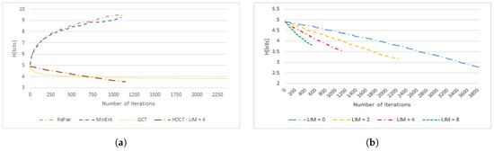
Figure 1.
Comparison of zero order entropy evolution over the paper5 file from the Calgary corpus. (a) Evolution of zero order entropy for different strategies; (b) evolution of zero order entropy for different values of the limit (LIM) in the strategy.
Both compression functions achieve a very similar resulting value of zero order entropy. The Re-Pair strategy begins with the highest growth of entropy, but the increase slows down with the number of iterations as the frequency of each consecutive digram drops. As will be discussed in Section 4.2.2, digrams consisting of symbols with a lower frequency will be preferred by MinEnt, because they will be able to achieve a larger decrease of entropic size, and their replacement brings less costs in the zero order entropy increase. This behavior can be observed especially in later iterations of the Re-Pair and MinEnt algorithms.
Both transformations reduce the value of zero order entropy. initially drops faster, but in the end, it significantly slows down. The application of the strategy achieves the lowest resulting value of entropy, and the interesting fact is that it decreases at an almost constant rate. The behavior of entropy evolution for different values of the limit in is presented in Figure 1b. The unrestricted case () shows us the bottom limit of zero order entropy reduction using the strategy.
3.3.3. Comparison of Entropic Size Evolution
The selection of the most frequent digram will produce the largest decrease of the number of symbols in each iteration. Surprisingly, the Re-Pair strategy does not necessarily have to converge to its minimum in the lower number of iterations than MinEnt. Figure 2 presents this behavior for the paper5 file of the Calgary corpus. Both approaches end with a similar number of symbols in the resulting message.
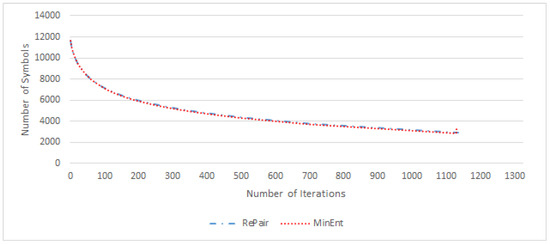
Figure 2.
Comparison of Re-Pair and MinEnt algorithms: evolution of the message size measured in the number of symbols over the paper5 file from the Calgary corpus.
The MinEnt strategy achieves the lowest entropic size of the message, and at each iteration, the entropic size of the message is lower than in the case of the Re-Pair strategy, see Figure 3. The overall efficiency depends on our ability to compress the resulting dictionary.
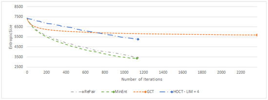
Figure 3.
Comparison of Re-Pair, MinEnt, and algorithms: evolution of the entropic message size measured in bits per byte over the paper5 file from the Calgary corpus.
A summary of different transformation strategies is provided in Table 2. A summary of compression functions is then given in Table 3. The least number of iterations was achieved by with ; this strategy also leads to the least final size , but it should be emphasized that the resulting entropic size of the message is a very pessimistic estimate, due to the construction of the size of dictionary entries.
Table 2.
The comparison of transformation strategies using different criteria: is the limiting size of the dictionary entry in bytes, i is the number of iterations; is the final entropy measured in bits; is the final entropic size measured in bytes; is the upper boundary on the amount of information needed to store one symbol to dictionary; and is the final size of the file given as the sum of the entropic size of the message and the size of the dictionary measured in bytes.
Table 3.
The comparison of compression strategies using different criteria: i is the number of iterations; is the size of the final alphabet; is the resulting size of the file measured as the number of symbols; is the final entropy measured in bits; is the final entropic size measured in bytes; is the average number of bits needed to store one phrase in the dictionary; and is the final size of the file given as the sum of the entropic size of the message and the size of the dictionary measured in bytes.
Even though the achieved results of both approaches are similar, we see that the resulting message size and alphabet size are lower in the case of MinEnt. The message size is given by the sum of the entropic size of the message and the size of the dictionary stored by interpolative encoding. Using values in the columns of Table 3, we express ; the term represents the size of the dictionary given as a product of the total number of iterations and the average number of bits needed to encode one iteration. See Table 4 and Table 5 for more results on files from the Calgary and Canterbury corpora.
Table 4.
The comparison of strategies using different criterions, i is the number of iterations, is the size of the final alphabet, is the resulting size of file measured as the number of symbols, is the final entropy measured in bits, is the final entropic size measured in bytes, is the average number of bytes needed to store one phrase into the dictionary and is the final size of the file given as the sum of entropic size of the message and the size of the dictionary measured in bytes.
Table 5.
The comparison of the strategies using different criteria: i is the number of iterations; is the size of final alphabet; is the resulting size of the file measured as the number of symbols; is the final entropy measured in bits; is the final entropic size measured in bytes; is the average number of bytes needed to store one phrase in the dictionary; and is the final size of the file given as the sum of entropic size of the message and the size of the dictionary measured in bytes.
4. Zero Order Entropy and Entropic Message Size Reduction
The primary purpose of context transformation and other derived transformations is to reduce the zero order entropy measured by Shannon’s entropy [2] defined in Equation (1). In this section, we shall show under what conditions the transformation and compression function reduces zero order entropy resp. the entropic size of the message. Suppose that is a zero order entropy of message m, and is a zero order entropy after a transformation T is applied. The conditions under which the following inequalities hold are the major subject of interest.
Let be a set of symbols whose frequencies before and after transformation differ, and is a set of symbols whose frequencies are intact. For transformations, the inequality (5) can be further restricted only to the set of symbols , since the terms containing symbols from subtract:
In the following paragraph, we will specify the forms of the set and the relations for the probabilities of its symbols after transformations, so that the change of entropy given by Equation (6) can be computed before any transformation actually occurs.
4.1. Transformation of Probabilities
We begin with the simplest case: suppose the context transformation . Since only the probabilities of symbols and will change, then , and it is sufficient to express probabilities only for and :
and:
In the case of the generalized context transformation , the set is identical, and the probabilities transform according to:
and:
In the last case of higher order transformation, the probabilities transform according to:
and:
In all cases, the set forms a binary alphabet. The following theorem then describes the condition for zero order entropy reduction:
Theorem 1.
Suppose the generalized context transformation . Let and be the probabilities of symbols before the transformation is applied, and let . After the transformation, the associated probabilities are , and . If , then the generalized context transformation T reduces entropy.
The proof of Theorem 1 is based on the properties of entropy when only two letters from alphabet are considered. Let , where , c is invariant, it does not change during the transformation. We can express one of these probabilities using the other one; for example, let ; this allows us to express the entropy function as a function of only one variable. A few examples of such functions are shown in Figure 4. The maximum value of the function is located in the value , and it has two minimums at zero and at c.
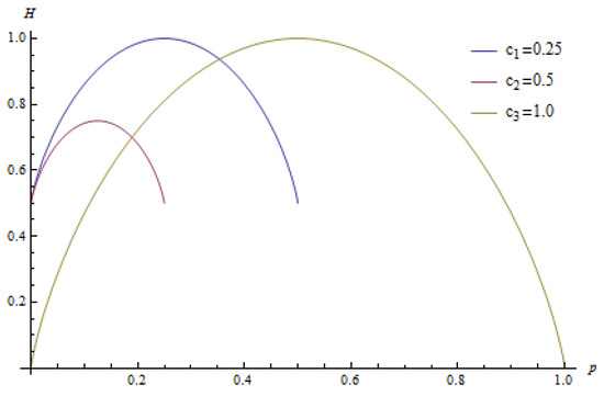
Figure 4.
The entropy of two letters with different .
Proof.
Since the entropy function for two different letters is defined on the interval and it is concave with a maximum at and minimums at zero and c, then has to be located on the interval ; but on that particular interval, the higher the maximum is, the lower the entropy is, so if we increase the maximum (or we can say increase the absolute value of the difference ), then the entropy will decrease. ☐
4.2. General Entropy Change Relations
In this section, we generalize the notion of zero order entropy change on the exchange of any two words. The solution is divided into three parts. The first part deals with the set of symbols whose frequency does not change before and after the substitution function is applied; the second part establishes relations for the set of symbols whose probability is changed, but their initial and final frequencies are non-zero; the third part discusses symbols introduced to and removed from the alphabet. Let be a set of removed symbols, and is a set of introduced symbols; then, we can split the sum in Equation (1), yielding:
The four sets of symbols in Equation (13) exhibit different behaviors under the substitution function, and they will be discussed in separate sections. The entropic size of the message can also be handled separately; let be a portion of entropy conveyed by symbols from alphabet , and let be particular portions of the entropic size of the message; then, we can split the resulting entropic size as we did before:
4.2.1. The First Part: Symbols Remaining Intact by the Substitution Function
We begin with symbols that are not part of either of the substituting words or . Suppose that the length of the message turns into some message of the size . Generally, , but in a special case of context transformations, these two quantities are equal. However, when the compression or expansion of the message occurs, the part of the Shannon equation will also change due to the change in the total number of symbols.
Suppose that the symbol x is initially in the message with the probability . This probability can be expressed using the frequency and the size of the message as:
Later, after the transformation was applied, the probability changes to:
where is a change of the message size. In the case of context transformations where the message size remains the same size, the probability remains the same, as well as the part of entropy formed by non-transformed symbols.
When the two probabilities are placed in relation by some stretching factor we arrange them into the form:
The factor (the introduction of is motivated by the properties of logarithms if we would actually stay with given by Equation (16), we would get logarithm . If instead, we express using (17), then the logarithm is in product form, and its arguments are single numbers ) can be expressed by substitution of in Equation (17) by the terms in Equations (15) and (16), leading to:
Then, the relation for zero order entropy after transformation will have the form:
The example of the behavior of of the intact part is visualized in Figure 5. When the compression of the message occurs, i.e., , then the zero order entropy of intact symbols increases. The less the probability is conveyed by symbols from , the more their zero order entropy is sensitive to the change of .
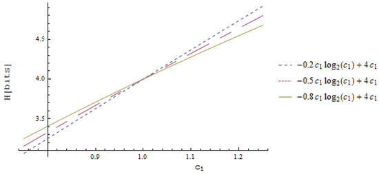
Figure 5.
The portion of entropy given by symbols from as a function of for the constant and .
The final entropic size is given as follows:
If we apply one of transformations, then , and as a consequence, ; the last term on the right will be zero due to , so Equation (20) tells us that the entropic size of the message carried by these symbols does not change during transformation. When is much smaller than , it is convenient to rewrite Equation (20) in terms of :
Corollary 1.
No compression function ever increases the entropic size of the part of the message consisting of intact symbols.
Proof.
The compression function has the value of larger than one, as a consequence , and so, . ☐
The equality in occurs when , i.e., when there are no intact symbols. When the expansion of the message occurs, then and the second term of Equation (20) on the right will change to a positive number. Expansion of the message leads to the increase of the entropic size; meanwhile, compression leads to the decrease of the entropic size of intact symbols.
In each iteration of the Re-Pair algorithm, the most frequent digram is selected. This corresponds to the selection of a digram with maximal value of , but it does not have to be the digram minimizing the entropic size of this part of the resulting message the most. Consider two digrams and , so that their frequencies are equal: ; replacing them with a new symbol yields the same stretching factor , but not necessarily . The larger reduction of the entropic size of a message will be achieved when compressed digrams or words consist of less frequent symbols.
4.2.2. The Second Part: Symbols Participating in the Substitution Function
In the second case, the frequencies of symbols and their total number will change. The equation for stretching factor will be derived in the following way:
The main difference in both cases is that is a constant; meanwhile, is a function of the particular symbol x.
where in the last step, we made the substitution: The rest of the derivation follows the derivation of Equation (19).
The behavior of Equation (23) for different values of is visualized in Figure 6. The substitution of less frequent symbols leads to a lower increase of zero order entropy.
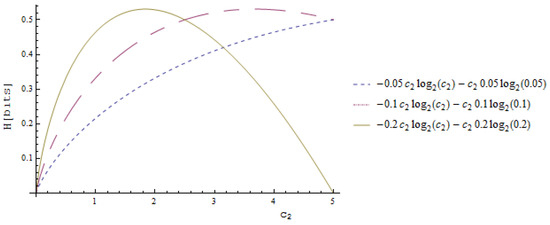
Figure 6.
Dependency of on different values of for three cases of .
The resulting entropic size simplifies given that:
yields:
We now analyze both terms in (25) from the perspective of different values of . We will be particularly interested in compression functions. We know that for compression function , symbols with , i.e., symbols whose frequency decreases, will have . The positivity or negativity of then depends on the value of product .
The case when has a solution , then . The term is always negative. The value of must be larger than to decrease the zero order entropy conveyed by symbol x, since then, and, as a consequence, .
The introduction of the absolute value in the middle step of the derivation of Inequality (26) is allowed since using compression functions values of and can only be negative. Suppose now that we have a digram , given that , and we replace it by the newly-introduced , then . The left part of Inequality (26) becomes equal to one, so Inequality (26) cannot be satisfied, and in this case will be negative and will always increase the amount of information carried by the symbols and .
Finally, we state the condition for the entropic size decrease:
Corollary 2.
The entropic size of the part of the message formed by symbol x decreases when:
Proof.
☐
4.2.3. Third Part: Introduced and Removed Symbols
We begin with symbol x, which is completely removed from the message, so that initially, , but . This case is trivial, and it has zero participation in the final value of the entropy and the entropic size of message. The remaining case we have to deal with is a case when initially symbol x has zero probability , but after substitution, its probability will increase to some . The final probability is given as:
Since the symbol x initially has zero participation in entropy and entropic size, it will always lead to the increase of both quantities. For the set of all such symbols, its portion on total entropy is then given by:
and the corresponding final entropic size will be given by:
It is important to remark that it does not make much sense to introduce more than one symbol in one substitution function, because both quantities would then add themselves twice.
4.3. Calculation of
At first glance, it seems that we need to evaluate all symbols to predict zero order entropy, but instead, it is possible to predict the exact change of the entropic size of the message after the application of the compression function by the evaluation of entropic sizes given by Equations (21), (25) and (30) dealing only with symbols . In the particular case of the Re-Pair algorithm, there are only two symbols whose frequency knowledge is sufficient to evaluate the change of the entropic size of the message; suppose a compression function so that , and , then the resulting entropic size is given as:
finally, for the Re-Pair, it holds that if , then , and all ’s in (31) turn into . If , then .
5. Conclusions
We described three types of transformations for the preprocessing of messages so that the zero order entropy of messages drops so the resulting message can be more efficiently encoded using zero order entropy compression algorithms like Huffman or arithmetic coding.
We presented relations that govern the change of the message size for transformations and compression functions. Transformations have the advantage that they do not modify the size of the alphabet, especially in the case of digram substitution used by Re-Pair and our proposal of the MinEnt strategy; the resulting size of the alphabet significantly grows, and it brings additional complexity in the storage of the entropy coding model, i.e., the storage of the output alphabet.
The MinEnt strategy selects digrams to be replaced by the minimal entropic size of the resulting message, and it is shown that in most cases, the resulting message size is smaller than the one achieved by Re-Pair. We also showed that the two algorithms follow slightly different execution paths, as MinEnt prefers digrams that consist of less frequent symbols; meanwhile, Re-Pair does not take this into consideration.
The compression functions take advantage of transformations as they achieve a better resulting compression ratio. In future work, we will focus on the storage of the dictionary that will be used in transformation algorithms, because this area can significantly improve the resulting compression ratio. Further, we will focus on the description of the relation between the entropy coding model of the final message and the size of the final alphabet.
Acknowledgments
This work was supported by the project SP2017/100 Parallel processing of Big Data IV, of the Student Grant System, VSB-Technical University of Ostrava. The costs for open access were covered.
Author Contributions
Michal Vasinek realized this work, proposed and developed the implementation of the , , and MinEnt algorithms. Jan Platos provided the guidance during the writing process and revised the paper.
Conflicts of Interest
The authors declare no conflict of interest.
Appendix A
The following sections present properties of transformations. Specifically for each type of transformation we will provide a proof of the inverse transformation existence. Further we will describe how the frequencies of symbols will be altered if the particular transformation is going to be applied.
Appendix A.1. CT—Proof of the Correctness
This theorem defines the inverse transformation of the context transformation:
Theorem A1.
The context transformation is inverse transformation of the context transformation .
Proof.
Let , if is inverse then the following must be true for any message m: . Suppose that we are passing message m from the end to the beginning and suppose that in positions i and digram is located, this digram is replaced by , the next pair of positions explored are and i, but their value is independent of the preceding replacement, because the replacement has taken place in position , so when is applied in position i it will find there the digram and reverts it back to . ☐
Other combinations of directions do not form a pair of transformation and its inverse. We give an example for each case showing this property: and over the message : but . Next consider and over the message : but . And in the last case let’s consider and over the message : but .
Let is a number of occurrences of particular digram in a message m, then the following corollary tells us how many digrams is introduced by context transformation :
Corollary A1.
Under assumption that the number of occurrences of digrams and after application of transformation is and .
Proof.
A proof is a consequence of Theorem A1, since each replacement is independent of each other and so each digram is replaced by leaving and . ☐
The corollary allows us to precisely predict not only the frequencies of the interchanged digrams and but also as a consequence the frequencies of individual symbols after transformation. The special case of transformations on a diagonal (see Definition A1) will be discussed in the next paragraph.
Appendix A.2. Diagonal Context Transformation
Diagonal transformation is a transformation where one of the digrams participating in the transformation is of the form . The resulting frequency of such a digram is unpredictable without knowledge of the distribution of all n-grams of the form , where , but we show that for any diagonal , it is possible to predict frequencies of symbols and . The problems with predictability arise from the repetition of symbols.
Definition A1.
Diagonal context transformation is a context transformation of the form .
Consider two transformations, and , if Corollary A1 would also be valid for diagonal transformations, then for instance in the case of , the frequency but this obviously is not true, instead we see that the new frequency of symbol is .
Suppose we have a message , then , we clearly see that the frequency and , because the number of digrams in a message is given by the length of the message minus one. We can now express the frequency of the newly introduced occurrences of digram as a sum of all sub-messages enclosed in m in the form , where for all . So we see that it is possible to precisely predict the change of frequency of , but it demands knowledge of the distribution of all enclosed sub-messages s.
From the other perspective, since each occurrence of digram in the former message is transformed into we can see that the frequency and .
Very similar behavior is observed in the second case of . The problem is in the repetition of the pattern , then and . Again without knowledge of all sub-messages t enclosed in m we cannot predict the exact change of frequency of neither digram nor , but since we know that each pair in the former message will be transformed to , we can again precisely predict frequencies of individual symbols and .
With the knowledge of the preceding discussion and of Corollary A1 we conclude that for any context transformation we are able to compute the frequency and corresponding probability of arbitrary symbol after application of any from the knowledge of initial distribution of symbols and digrams. In [26] we showed that under certain conditions it is possible to process several context transformations simultaneously.
Appendix A.3. GCT—Frequencies Alteration
Corollary A2.
Under assumption that , and the number of occurrences of digrams and after application of transformation is and .
Proof.
Since each digram resp. is replaced by resp. , and neither of the digrams influence the transformation of the other, their frequencies must interchange. ☐
Appendix A.4. Generic Transformation—Proof of Correctness
Generic transformation exchanges any two digrams. In the design of algorithms, we prefer over since the space from which generic transformations are selected is in this case of order the and when alphabets of the large size are dealt with, the search in such a space would be computationally very expensive.
Definition A2.
Generic transformation (GT) is the mapping , Σ is the alphabet of the input message w and n is the length of the input message, that exchanges all digrams for digram and vice-versa.
The inverse transformation of and is defined by the following theorem:
Theorem A2.
Generic transformation resp. is the inverse of generic transformation resp.
Proof.
First, we show that it is sufficient to prove that for any string , it holds that , where and . Suppose that x is located in position p then for digrams d in positions and it holds that . So the first possible application of GT can occur in positions and and these are independent, i.e., non-overlapping.
Next, we show that each replacement made in the forward transformation will be reverted back by inverse transformation. Take for example transformation the transformation is applied in the right to left direction. The last applied forward transformation in positions replaces for instance digram for leaving , the inverse transformation, by definition the same transformation applied in the opposite direction, reverts digram back to . Now consider any triplet of positions in a transformed message, the input of the inverse transformation in is dependent on the result of the inverse transformation in the preceding pair of positions, but as we saw the first applied inverse reverted digram back correctly so the state in positions is exactly like the one of the state left by forward transformation in these positions, so any other digram will be reverted back correctly, because every preceding application of the inverse leaves the state of the digram in the state that was left by the forward transformation and this digram is trivially reverted back to initial state. The same rules are valid for in the opposite direction, since the transformation , where is a mirror message of m. ☐
Appendix A.5. HOCT—Proof of the Correctness
The following trivial Lemma will help us to formulate a theorem about inverse transformation to :
Lemma A1.
Let is a higher order context transformation over the input message m, given that we possess the knowledge of w and positions , then .
Proof.
Because we don’t have to pass through the whole message either in the forward or inverse transformation case, but only through the set of positions , then the symbol in position , for instance will switch by to and by repeated application of it reverts back to . ☐
The Lemma A1 is trivial but comes into play when is a product of some other higher order context transformation, i.e., the one with an order lower by one.
Theorem A3.
Let and are two higher order context transformations. Let be a transformation composition of two higher order context transformations over input message m. Then , such that then the transformation composition is the inverse transformation of T.
Several remarks to the formulation of Theorem A3: Transformations and are applied over two consecutive states of the message. The positions correspond to the positions , since sub-messages have been replaced by in the application of . The inverse transformation by is applied instead over positions , since these positions have already been reverted back by .
The proof is based on the restriction that , , it can be viewed as we would split the input message m to sub-messages separated by . For instance, suppose that is a space character in ordinary text, since, by Definition 3, no other character in w can be a space character, it follows that the possible transformations are being applied on words following the space character. Now using the fact that is enclosed by , i.e., they do not overlap, allows us to handle each sub-message independently.
Proof.
For the two sets of positions, it holds that , because elements of the former are predecessors of the latter and s does not overlap. The locations of w in m and are identical as they were not modified during , i.e., . When we apply again it will simply revert the symbols in positions given by back according to Lemma A1 yielding the message state . In the forward transformation was applied over positions of , but these are the former positions of , that are already transformed back by the application of , so is equal to and when is applied over positions it exchanges symbols and and eventually yields m. ☐
The recursive application of Theorem A3 leads to the conclusion that this process can be repeated until there is no other pair of symbols then these containing as one of the symbols or or we simply reach the end of the message.
Corollary A2 about the prediction of frequencies in the case of is also applicable in the case of , because the principle that the exact number of replacements is known is also valid and we are able to precisely compute the future probabilities of symbols before the arbitrary is applied.
If we implement the inverse algorithm as a sequential algorithm operating in the left-right manner, it is possible to have one of the transformation symbols if is equal to . Suppose the following example: , , and yielding the output message . Now applying inverse transformation sequentially from left to right, we first replace by yielding , then applying replacement for yielding , now because there is no other transformation that is induced from we know that the next a symbol is and we can repeat the preceding process again starting from this a. The sufficient condition for the introduction of as the transformation symbol or is that w contains no other in , , because the inverse process removes all introduced symbols from the transformed message during left to right sequential inverse transformation.
References
- Cover, T.M.; Thomas, J.A. Elements of Information Theory (Wiley Series in Telecommunications and Signal Processing); Wiley-Interscience: New York, NY, USA, 2006. [Google Scholar]
- Shannon, C.E. A Mathematical Theory of Communication. Bell Syst. Tech. J. 1948, 27, 379–423. [Google Scholar] [CrossRef]
- Huffman, D.A. A Method for the Construction of Minimum-Redundancy Codes. Proc. Inst. Radio Eng. 1952, 40, 1098–1101. [Google Scholar] [CrossRef]
- Witten, I.H.; Neal, R.M.; Cleary, J.G. Arithmetic Coding for Data Compression. Commun. ACM 1987, 30, 520–540. [Google Scholar] [CrossRef]
- Charikar, M.; Lehman, E.; Lehman, A.; Liu, D.; Panigrahy, R.; Prabhakaran, M.; Sahai, A.; Shelat, A. The Smallest Grammar Problem. IEEE Trans. Inf. Theory 2005, 51, 2554–2576. [Google Scholar] [CrossRef]
- Nevill-Manning, C.G. Inferring Sequential Structure. Ph.D. Thesis, University of Waikato, Hamilton, New Zealand, May 1996. [Google Scholar]
- Nevill-Manning, C.G.; Witten, I.H. Identifying Hierarchical Structure in Sequences: A Linear-time Algorithm. J. Artif. Int. Res. 1997, 7, 67–82. [Google Scholar]
- Kieffer, J.C.; Yang, E.-H. Grammar Based Codes: A New Class of Universal Lossless Source Codes. IEEE Trans. Inf. Theory 2000, 46, 737–754. [Google Scholar] [CrossRef]
- Ziv, J.; Lempel, A. Compression of individual sequences via variable-rate coding. IEEE Trans. Inf. Theory 1978, 24, 530–536. [Google Scholar] [CrossRef]
- Yang, E.; He, D. Efficient universal lossless data compression algorithms based on a greedy sequential grammar transform 2. With context models. IEEE Trans. Inf. Theory 2003, 49, 2874–2894. [Google Scholar] [CrossRef]
- Gage, P. A New Algorithm for Data Compression. C Users J. 1994, 12, 23–38. [Google Scholar]
- Nakamura, H.; Marushima, S. Data Compression by Concatenation of Symbol Pairs. In Proceedings of the IEEE International Symposium on Information Theory and Its Applications, Paris, France, 13–17 September 1996; pp. 496–499. [Google Scholar]
- Larsson, N.J.; Moffat, A. Off-line dictionary-based compression. Proc. IEEE 2000, 88, 1722–1732. [Google Scholar] [CrossRef]
- Claude, F.; Farina, A.; Navarro, G. Re-Pair Compression of Inverted Lists. arXiv 2009. [Google Scholar]
- Masaki, T.; Kida, T. Online Grammar Transformation Based on Re-Pair Algorithm. In Proceedings of the Data Compression Conference (DCC), Snowbird, UT, USA, 29 March–1 April 2016; pp. 349–358. [Google Scholar]
- Grassberger, P. Data Compression and Entropy Estimates by Non-sequential Recursive Pair Substitution. Physics 2002. [Google Scholar]
- Calcagnile, L.M.; Galatolo, S.; Menconi, G. Non-sequential recursive pair substitutions and numerical entropy estimates in symbolic dynamical systems. arXiv 2008. [Google Scholar]
- Navarro, G.; Russo, L. Re-pair Achieves High-Order Entropy. In Proceedings of the Data Compression Conference, DCC 2008, Snowbird, UT, USA, 25–27 March 2008; p. 537. [Google Scholar]
- Vasinek, M.; Platos, J. Entropy Reduction Using Context Transformations. In Proceedings of the Data Compression Conference (DCC), Snowbird, UT, USA, 26–28 March 2014; p. 431. [Google Scholar]
- Vasinek, M.; Platos, J. Generalized Context Transformations—Enhanced Entropy Reduction. In Proceedings of the Data Compression Conference (DCC), Snowbird, UT, USA, 7–9 April 2015; p. 474. [Google Scholar]
- Vasinek, M.; Platos, J. Higher Order Context Transformations. arXiv 2017. [Google Scholar]
- Kida, T.; Matsumoto, T.; Shibata, Y.; Takeda, M.; Shinohara, A.; Arikawa, S. Collage System: A Unifying Framework for Compressed Pattern Matching. Theor. Comput. Sci. 2003, 298, 253–272. [Google Scholar] [CrossRef]
- González, R.; Navarro, G. Compressed Text Indexes with Fast Locate. In Proceedings of the 18th Annual Conference on Combinatorial Pattern Matching, CPM’07, London, ON, Canada, 9–11 July 2007; Springer: Berlin/Heidelberg, Germany, 2007; pp. 216–227. [Google Scholar]
- Claude, F.; Farina, A.; Navarro, G. Re-Pair compression of inverted lists. arXiv 2009. [Google Scholar]
- Vasinek, M. Kontextove Mapy a Jejich Aplikace. Master’s Thesis, Vysoka Skola Banska—Technicka Univerzita Ostrava, Ostrava, Czech Republic, 2013. [Google Scholar]
- Vasinek, M.; Platos, J. Parallel Approach to Context Transformations. Available online: http://ceur-ws.org/Vol-1343/paper4.pdf (accessed on 11 May 2017).
© 2017 by the authors. Licensee MDPI, Basel, Switzerland. This article is an open access article distributed under the terms and conditions of the Creative Commons Attribution (CC BY) license (http://creativecommons.org/licenses/by/4.0/).