Entropy Conditions Involved in the Nonlinear Coupled Constitutive Method for Solving Continuum and Rarefied Gas Flows

Abstract

The numerical study of continuum-rarefied gas flows is of considerable interest because it can provide fundamental knowledge regarding flow physics. Recently, the nonlinear coupled constitutive method (NCCM) has been derived from the Boltzmann equation and implemented to investigate continuum-rarefied gas flows. In this study, we first report the important and detailed issues in the use of the H theorem and positive entropy generation in the NCCM. Importantly, the unified nonlinear dissipation model and its relationships to the Rayleigh–Onsager function were demonstrated in the treatment of the collision term of the Boltzmann equation. In addition, we compare the Grad moment method, the Burnett equation, and the NCCM. Next, differences between the NCCM equations and the Navier–Stokes equations are explained in detail. For validation, numerical studies of rarefied and continuum gas flows were conducted. These studies include rarefied and/or continuum gas flows around a two-dimensional (2D) cavity, a 2D airfoil, a 2D cylinder, and a three-dimensional space shuttle. It was observed that the present results of the NCCM are in good agreement with those of the Direct Simulation Monte Carlo (DSMC) method in rarefied cases and are in good agreement with those of the Navier–Stokes equations in continuum cases. Finally, this study can be regarded as a theoretical basis of the NCCM for the development of a unified framework for solving continuum-rarefied gas flows.

1. Introduction

The numerical study of continuum-rarefied gas flows is of great interest because it can provide fundamental knowledge regarding flow physics and provide a theoretical tool to precisely predict the aerodynamic or aerothermodynamic performance of hypersonic vehicles and/or Micro-Electro-Mechanical Systems [1,2,3,4]. For more than 150 years, the Navier–Stokes–Fourier (NSF) equations have been accepted as the model that describes flow dynamics. Unfortunately, the NSF equations have serious limitations in capturing the correct flow physics under highly nonequilibrium conditions, such as for rarefied gas [5]. For the investigation of rarefied and/or micro-gas flows, much effort has been put into the development of computational models beyond the NSF framework. The models can be classified into two categories: the full kinetic model and the fluid dynamics model. The most successful methods in the former category are the direct simulation Monte Carlo (DSMC) [6,7,8,9] and Lattice Boltzmann Methods (LBM) [10,11,12,13,14], and they have been extensively used for the computation of rarefied and/or micro-scale gas flows. Although the Direct Simulation Monte Carlo (DSMC) method is commonly used in the investigation of rarefied gas flows, it has unacceptable memory demands in near continuum states because it uses simulated molecules to model the movement of molecules and the collision of gas flows. Great progress has been made in the development of LBM to remove its capability limit in complex far-from-equilibrium flows, of which the regularized LBM work done by Montessori and Succi is typically representative [12]. Importantly, LBM has been successfully extended to investigate turbulent gas flows by Chen and Succi [15]. On the other hand, the fluid dynamics models are based on the hyperbolic conservation laws and nonconserved variables appearing in the conservation laws, the latter being determined by their evolution equations which can be derived with the help of the Boltzmann equation. Up to present, several models have been developed for the latter category. This category may be subdivided into a few classes: in one of them, the Burnett-type equations [16,17] are used for devising computational models; in another, Grad moment equations [18] and 13 moment equations [19,20] are employed in conjunction with extended thermodynamics; and in still another, the Eu moment equations that serve as the basis of the generalization of thermodynamics [21,22] have been used in a manner consistent with the laws of thermodynamics at every order of approximation employed. Recently, Eu moment equations have been well-developed by Myong to investigate stiff hypersonic nonequilibrium gas flows [22,23,24,25,26].

Recently, we reported and validated the nonlinear coupled constitutive method (NCCM) for the development of a unified scheme for modelling continuum-rarefied gas flows [4]. It can be regarded as another option to treat EU equations. In addition, we tried to extend the NCCM to investigate turbulence and have made great progress recently. In the NCCM, the conservation laws of mass, momentum, and energy are derived from the Boltzmann equation via the EU method [21,22] and are similar to those of the NSF equations. However, nonconserved variables associated with thermal nonequilibrium, such as the shear stress tensor and the heat flux vector, are described by the evolution equations. These variables are quite different from those in the NSF equations in conjunction only with the linear constitutive relations of the gradients of velocity and temperature. In the present study, we first provide the theoretical basis of the NCCM, particularly for positive entropy generation and the unified nonlinear dissipation model according to Eu method. This study can be regarded as an extension of the previous study of the NCCM and Eu method, in which we focus on the numerical scheme for solving NCCM equations and its validation in typical continuum-rarefied gas flows.

2. Boltzmann Equations and Entropy Transport Equation

2.1. Boltzmann Equations and the Feature of Irreversibility

The distribution function f_i denotes the probability of finding a particle of species $i$ in the range of $v_i+d{v}_i$ and $r_i+d{r}_i$ at time $t$. The Boltzmann equation yields the evolution equation for $f_i$,

$$\frac{\partial f_i}{\partial t}+v_i\cdot \nabla f_i+F_i\cdot {\nabla }_{v_i}{f}_i=R\left(f_i\right).$$

(1)

In this equation, $R\left(f_i\right)$ is the collision term, $F_i$ is the external force, and $v_i$ is the velocity of a particle of species $i$. We can simply rewrite $R\left(f_i\right)$ in the following form:

$$\begin{array}{l}R\left(f_i\right)={\displaystyle \sum _{j=1}^{r}C\left(f_i,f_j\right)}\\ C\left(f_i,f_j\right)={\displaystyle \int d}{v}_j{\displaystyle {\int }_0^{2\pi }d\varphi }{\displaystyle {\int }_0^{\infty }b{g}_{ij}[f_i^{*}(v_i^{*},r;t)f_j^{*}(v_j^{*},r;t)-f_i(v_i,r;t)f_j(v_j,r;t)]db}\end{array}$$

(2)

where $b$ is the impact parameter and it is the distance between the two parallel lines passing through the center of the collision molecule, $r$ is the number of species, and $g_{ij}=\left|v_i-v_j\right|$ is the relative speed. $C\left(f_i,f_j\right)$ is the Boltzmann collision integral, and it accounts for the decrease and increase in probability caused by collisions and reverse collisions, respectively [21].

If we reverse time $t$ to $-t$, then the velocities must also be reversed, and the Boltzmann equation takes the following form:

$$\left({\partial }_{-t}+\left(-v_i\right)\cdot {\nabla }_i+F_i\cdot {\nabla }_{-v_i}\right)f_i\left(-v_i,r;-t\right)={\displaystyle \sum _{j=1}^{r}C\left(f_i{\left(-v_i,r;-t\right)}_i,f_j\left(-v_j,r;-t\right)\right)}.$$

(3)

In this equation, we have

$$\begin{array}{l}C\left(f_i{\left(-v_i,r;-t\right)}_i,f_j\left(-v_j,r;-t\right)\right)\\ ={\displaystyle \int d}{v}_j{\displaystyle {\int }_0^{2\pi }d\varphi }{\displaystyle {\int }_0^{\infty }b{g}_{ij}[f_i(-v_i,r;-t)f_j(-v_j,r;-t)-f_i^{*}(-v_i^{*},r;-t)f_j^{*}(-v_j^{*},r;-t)]db}\end{array}.$$

(4)

Because the time is reversed, the positions of the post-collision and pre-collision terms are exchanged in Equation (4). This reversion transforms the Boltzmann collision integral into the negative of the original one before the time reversal. Thus, the time reversal invariance is broken because of the presence of the Boltzmann collision integral. As a result, in the sense that the time reversal invariance is broken, the Boltzmann equation is irreversible and is consequently expected to describe the irreversible macroscopic process towards equilibrium. This feature expression is very important and is represented in a more useful form via the H theorem and the Entropy balance equation [21].

2.2. H Theorem and Entropy Balance Equation

The H function was introduced by Boltzmann to show that the solution of the Boltzmann equation generally approaches a unique equilibrium solution. In addition, this function’s time derivative can be proved to decrease to zero as the system approaches equilibrium. Moreover, this H function was found to be closely related to the entropy introduced by Clausius. Thus, the nonequilibrium entropy of the system is defined by [21]:

$$S(t)=-k_B{\displaystyle \sum _{i=1}^r{\displaystyle \underset{V}{\int }d}}r{\displaystyle \int d}{v}_i{f}_i(v_i,r;t)(\ln f_i-1).$$

(5)

The H theorem states that

$$\frac{dS}{dt}\ge 0.$$

(6)

If we use the local equilibrium temperature $T_e$ to replace the temperature $T$ in the Maxwell–Boltzmann distribution function, then the local equilibrium distribution function can be obtained:

$$f_i^0(v_i,r)=n_i^0{(m_i/2\mathsf{\pi }{k}_B{T}_e)}^{3/2}\exp [-(\frac{1}{2}{m}_i{\nu }_i^2+m_i{\Psi }_i(r))/k_B{T}_e].$$

(7)

Thus, the local equilibrium entropy can also be expressed by

$$S_e(t,f_i^0)=-k_B{\displaystyle \sum _{i=1}^r{\displaystyle \underset{V}{\int }d}}r{\displaystyle \int d}{v}_i{f}_{{}_i}^0(v_i,r;t)(\ln f_{{}_i}^0-1).$$

(8)

Furthermore, the nonequilibrium entropy can be defined by

$$S_n(t)=S(t,f_i)-S_e(t,f_i^0)=-k_B{\displaystyle \sum _{i=1}^r{\displaystyle \underset{V}{\int }d}}r{\displaystyle \int d}{v}_i[f_i\ln (f_i/f_i^0)-f_i+f_i^0].$$

(9)

By the well-known inequality,

$$y\ln (y/x)-y+x\ge 0$$

(10)

We conclude that

$$S_n(t)=S(t,f_i)-S_e(t,f_i^0)\le 0.$$

(11)

In other words, the entropy increases towards the equilibrium entropy, as dictated by the second law of thermodynamics. By differentiating $S_n(t)$ as a function of time, we obtain

$$\frac{d}{dt}{S}_n=-k_B{\displaystyle \sum _{i=1}^r{\displaystyle \underset{V}{\int }d}}r{\displaystyle \int d}{v}_i[{\partial }_t{f}_i\ln (f_i/f_i^0)].$$

(12)

Substituting the Boltzmann equation and proceeding in the same manner as that for the proof of the H theorem, we find

$$\frac{d}{dt}{S}_n\ge 0.$$

(13)

This finding indicates that the nonequilibrium entropy increases as the system approaches equilibrium. In addition, this feature can be expressed in the latter entropy balance equation.

We define the entropy density $\zeta$ by the formula

$$\rho \zeta =-k_B{\displaystyle \sum _{i=1}^r{\displaystyle \int d}{v}_i{f}_i(\ln f_i-1)=\langle f_i(\ln f_i-1)\rangle }$$

(14)

where $\zeta$ is the entropy per unit mass of the gas, and the total entropy can be obtained by integrating $\rho \zeta$ over the volume. By differentiating $\rho \zeta$ over time and using the Boltzmann equation on the right hand, the entropy balance equation can be obtained:

$$\rho \frac{d}{dt}\zeta =-\nabla \cdot J_s(r,t)+{\sigma }_{ent}(r,t)$$

(15)

where $J_s(r,t)$ is the entropy flux, and ${\sigma }_{ent}(r,t)$ is the entropy production. Next, the same procedure as that used to prove the H theorem can be applied to show that the entropy production is positive:

$$\begin{array}{l}{\sigma }_{ent}(r,t)=-k_B{\displaystyle \sum _{i=1}^r{\displaystyle \sum _{j=1}^r\langle \ln f_{i}C\left(f_i,f_j\right)\rangle }}\\ =\frac{1}{4}{k}_B{\displaystyle \sum _{i=1}^r{\displaystyle \sum _{j=1}^r{\displaystyle \int d{v}_i}{\displaystyle \int d{v}_j}{\displaystyle {\int }_0^{2\pi }d\varphi }\times {\displaystyle {\int }_0^{\infty }b{g}_{ij}\ln (f_i^{*}{f}_j^{*}/f_i{f}_j)(f_i^{*}{f}_j^{*}-f_i{f}_j)db}}}\ge 0\end{array}.$$

(16)

Therefore, the entropy balance equation has a positive source for entropy, i.e., the source creates entropy. The statistical expression for ${\sigma }_{ent}(r,t)$ suggests that entropy is created through numerous, random collisions of the particles in the gas because entropy production is intimately associated with energy dissipation. In addition, the energy dissipation may be regarded as a result of particle collisions that occur incessantly and randomly in the gas flow.

From the discussion above, one can conclude that the Boltzmann equation is irreversible in the nonequilibrium state. In addition, this feature can be expressed by the H theorem and entropy production. Meanwhile, the entropy production ${\sigma }_{ent}(r,t)$ is related to the collision term of the Boltzmann equation [21]. Moreover, this production is also associated with energy dissipation. The treatment of the collision term of the Boltzmann equation requires the identification of a model of energy dissipation.

3. Nonlinear Coupled Constitutive Method

3.1. Conservation Laws in the NCCM

The Boltzmann equation fulfils the requirements of the mass, momentum, and energy conservation laws. By differentiating the densities of mass, momentum, and energy, the conservation equations of gas flows can be obtained:

$$\begin{array}{l}\frac{\partial \rho }{\partial t}+\nabla \cdot \rho u=0\\ \frac{\partial \rho u}{\partial t}+\nabla \cdot (\rho uu+P)-\rho F=0\\ \frac{\partial \rho E}{\partial t}+\nabla \cdot (Q+\rho Eu)+P:\nabla u-{\displaystyle \sum _{i=1}^r\left(J_i\cdot F_i\right)=0}.\end{array}$$

(17)

In this equation, P is the stress tensor and is defined by $P=pI+\Delta \mathrm{I}+П$. $F_i$ is the external force per unit mass. In the gas flows, the external force is usually omitted. Thus, the conservation laws are simplified into [22,23,24,25,26]:

$$\begin{array}{l}\frac{\partial \rho }{\partial t}+\nabla \cdot \rho u=0\\ \frac{\partial \rho u}{\partial t}+\nabla \cdot (\rho uu+P)=0\\ \frac{\partial \rho E}{\partial t}+\nabla \cdot (Q+\rho Eu)+P:\nabla u=0.\end{array}$$

(18)

In this equation, P and Q are nonconservation variables with molecular expressions that do not yield a collisional invariant.

3.2. Evolution Equations of the Nonconservation Variables in NCCM

To derive the evolution equations for the nonconservation variables, we must define the velocity moment of order $l$

$${ℝ}_i^{\left(abc\dots l\right)}=\langle m_i{\ell }_{ia}{\ell }_{ib}{\ell }_{ic}\dots {\ell }_{il}{f}_i\left(v_i,r,t\right)\rangle .$$

(19)

Next, differencing this moment with time, we have

$$\begin{array}{ll}\frac{\partial }{\partial t}{ℝ}_i^{\left(abc\dots kl\right)}=& -{\partial }_t{u}_a{ℝ}_i^{\left(bc\dots l\right)}-{\partial }_t{u}_b{ℝ}_i^{\left(ac\dots l\right)}-{\partial }_t{u}_c{ℝ}_i^{\left(abd\dots l\right)}-\dots \\ & -{\partial }_t{u}_l{ℝ}_i^{\left(abc\dots k\right)}+\langle m_i{\ell }_{ia}{\ell }_{ib}{\ell }_{ic}\dots {\ell }_{il}{\partial }_t{f}_i\rangle \end{array}$$

(20)

The last collision term of Equation (20) is given by:

$$\begin{array}{lll}{S}_{ab\dots kl}& =& \langle m_i{\ell }_{ia}{\ell }_{ib}{\ell }_{ic}\dots {\ell }_{il}{\partial }_t{f}_i\rangle =\langle m_i{\ell }_{ia}{\ell }_{ib}{\ell }_{ic}\dots {\ell }_{il}{}_i({\displaystyle \sum _{j=1}^{r}C\left(f_i,f_j\right)}-v_i\cdot \nabla f_i-F_i\cdot {\nabla }_{v_i}{f}_i)\rangle \\ & =& -\left(u\cdot \nabla u_a\right){ℝ}_i^{\left(bc\dots l\right)}-\left(u\cdot \nabla u_b\right){ℝ}_i^{\left(ac\dots l\right)}-\left(u\cdot \nabla u_c\right){ℝ}_i^{\left(abd\dots l\right)}\\ & & -......-\left(u\cdot \nabla u_l\right){ℝ}_i^{\left(ab\dots k\right)}-{ℝ}_i^{\left(\cdot bc\dots l\right)}\cdot \nabla u_a-{ℝ}_i^{\left(a\cdot c\dots l\right)}\cdot \nabla u_b\\ & & -{ℝ}_i^{\left(ab\cdot d\dots l\right)}\cdot \nabla u_c-......-{ℝ}_i^{\left(abc\dots k\cdot \right)}\cdot \nabla u_l+F_{ia}{ℝ}_i^{\left(bc\dots l\right)}\\ & & +F_{ib}{ℝ}_i^{\left(ac\dots l\right)}+F_{ic}{ℝ}_i^{\left(abd\dots l\right)}+......F_{il}{ℝ}_i^{\left(abc\dots k\right)}\\ & & -\nabla \cdot \left({ℝ}_i^{\left(\cdot ab\dots l\right)}+u{ℝ}_i^{\left(ab\dots l\right)}\right)+{\Lambda }_i^{\left(ℝ\right)\left(abc\dots kl\right)}\end{array}.$$

(21)

In this equation, ${\Lambda }_i^{\left(ℝ\right)\left(abc\dots kl\right)}={\displaystyle \sum _{j-1}^r\langle m_i{\ell }_{ia}{\ell }_{ib}{\ell }_{ic}\dots {\ell }_{il}C\left(f_i,f_j\right)\rangle }.$

Finally, the derivative of the velocity moment can be obtained:

$$\begin{array}{ll}\frac{\partial }{\partial t}{ℝ}_i^{\left(abc\dots kl\right)}=& -\nabla \cdot \left({ℝ}_i^{\left(\cdot ab\dots l\right)}+u{ℝ}_i^{\left(abc\dots l\right)}\right)-{{\displaystyle \sum _{\mathrm{all} \mathrm{terms}}\left(\frac{du}{dt}\right)}}_a{ℝ}_i^{\left(bc\dots l\right)}\\ & -{\displaystyle \sum _{\mathrm{all} \mathrm{terms}}{ℝ}_i^{\left(\cdot bc\dots l\right)}}\cdot \nabla u_a+{\displaystyle \sum _{\mathrm{all} \mathrm{terms}}{F}_{ia}}{ℝ}_i^{\left(bc\dots l\right)}\\ & +{\Lambda }_i^{\left(ℝ\right)\left(abc\dots kl\right)}\end{array}$$

(22)

Substituting the stress tensor and the heat flux term into Equation (22), we have

$$P={\displaystyle \sum _{i=1}^r\langle m_i{\ell }_i{\ell }_i{f}_i(v_i,r;t)\rangle }Q={\displaystyle \sum _{i=1}^r{Q}_i}={\displaystyle \sum _{i=1}^r\langle \frac{1}{2}{m}_i{\ell }_i^2{\ell }_i{f}_i(v_i,r;t)\rangle }.$$

Next, we also obtain the transport equation of the stress tensor and the heat flux:

$$\begin{gathered} \begin{array}{ll}\frac{\partial }{\partial t}{P}_i=& -\nabla \cdot \left({\phi }_i^{\left(3\right)}+u{P}_i\right)-\left(d_{t}u{J}_i+J_i{d}_{t}u\right)-\left[P_i\cdot \nabla u+{\left(\nabla u\right)}^t\cdot P_i\right]\\ & +\left(F_i{J}_i+J_i{F}_i\right)+{\Lambda }_i^{\left(P\right)}\end{array} \\ \begin{array}{ll}\frac{\partial }{\partial t}{Q}_i=& -\nabla \cdot \left({\phi }_i^{\left(4\right)}+u{Q}_i\right)-d_{t}u\cdot \left(P_i+{\rho }_i{\ell }_{i}U\right)-{\phi }_i^{\left(3\right)}:\nabla u-Q_i\cdot \nabla u\\ & +F_i\cdot \left(P_i+{\rho }_i{\ell }_{i}U\right)+{\Lambda }_i^{\left(Q\right)}\end{array}. \end{gathered}$$

(23)

In this equation,

$$\begin{array}{l}{\phi }_i^{\left(3\right)}\equiv \langle m_i{\ell }_i{\ell }_i{\ell }_i{f}_i\rangle \\ {\phi }_i^{\left(4\right)}\equiv \langle \frac{1}{2}{m}_i{\ell }_i^2{\ell }_i{\ell }_i{f}_i\rangle \\ {\Lambda }_i^{\left(P\right)}={\displaystyle \sum _{j=1}^r\langle m_i{\ell }_i{\ell }_{i}C\left(f_i,f_j\right)\rangle }\\ {\Lambda }_i^{\left(Q\right)}={\displaystyle \sum _{j=1}^r\langle \frac{1}{2}{m}_i{\ell }_i^2{\ell }_{i}C\left(f_i,f_j\right)\rangle }\end{array}.$$

(24)

In addition, the external force is usually omitted. Moreover, it can be seen that there are four terms in these transport equations: the derivative with time, the gradient of high-order terms, and the flux and collision parts. Usually, we use the viscous stress and the excess normal stress to replace the stress tensor. For this purpose, the following formulations should be defined in the molecular expressions for the moments:

$$h_i^{(1)}={[m_i{\ell }_i{\ell }_i]}^{(2)}{h}_i^{(2)}=\frac{1}{3}{m}_i{\ell }_i^2-p_i/n_i{h}_i^{(3)}=(\frac{1}{2}{m}_i{\ell }_i^2+m_i{\Psi }_i-\widehat{h}{m}_i){\ell }_i$$

(25)

when the traceless part of the stress tensor is averaged over velocity, we denote them by the symbol ${\Phi }_i^{(a)}$

$${\Phi }_i^{(a)}=\langle h_i^{(a)}{f}_i(v_i,r;t)\rangle$$

(26)

where $a=1,2,3$, and $i=1,2,3,\dots ,n$. The meaning of the term ${\Phi }_i^{(a)}$ is as follows:

$${\Phi }_i^{(1)}={П}_i={[P_i]}^{(2)},{\Phi }_i^{(2)}={\Delta }_i=\frac{1}{3}\mathrm{T}\mathrm{r}{P}_i-p_i,{\Phi }_i^{(3)}=Q_i.$$

(27)

Thus, the transport equation of nonconservation variables can be obtained:

$$\rho \frac{d\left({\Phi }^{\left(\alpha \right)}/\rho \right)}{dt}+\nabla \cdot {\psi }^{\left(\alpha \right)}={\Lambda }_k+Z_k.$$

(28)

Here, ${\Lambda }_k$ denotes the collision term and can be expressed as

$${\Lambda }_k={\displaystyle \sum _{j=1}^r\langle h_i^{(a)}C(f_i,f_j)\rangle }.$$

(29)

3.3. Treatment of the Distribution Function in the Boltzmann Equation

At this stage, the most important work remaining is determining how to treat the collision term. The first step is the definition of the distribution function. The following primary concepts were implemented in this definition.

(1)

The definition of the distribution function from nonequilibrium to equilibrium is weak in form and dynamic. In other words, the distribution function has no exact and specific expression in the process of nonequilibrium.

(2)

The distribution function should fulfil not only the conservations of mass, momentum, and energy, but also the H theorem and positive entropy generation.

To fulfill the abovementioned rules and essential construction of the thermodynamic theory of irreversible processes, the definition of the distribution function is expressed via Eu Methods [17] as follows:

$$f_i=\exp [-\frac{1}{k_{\mathrm{B}}T}(H_i+H_i^{(1)}-{\mu }_i)].$$

(30)

In this equation,

${\ell }_i=v_i-u$ denotes the thermal motion velocity.

${\Psi }_i(r)$ denotes the potential energy.

$H_i=\frac{1}{2}{m}_i{\ell }_i^2+m_i{\Psi }_i(r)$

$H_i^{(1)}={\displaystyle \sum X_i^{(\alpha )}\odot h_i^{(\alpha )}}$

$h^{(\alpha )}$ is the molecular expressions for the moments of the nonequilibrium variable, and $X_{\alpha }$ denotes the weighting coefficient.

${\mu }_i$ denotes the following factor:

$$\exp (-\frac{1}{k_{B}T}{\mu }_i)=n_i^{-1}\langle \exp [-\frac{1}{k_{B}T}(H_i+H_i^{(1)})]\rangle .$$

(31)

In addition, in Equation (30), $H_i$ can be regarded as the local equilibrium, $H_i^{(1)}$ denotes the nonequilibrium condition, and ${\mu }_i$ connects the local equilibrium and nonequilibrium conditions to fulfill the conservation laws and positive entropy generation.

The advantage of this exponential form of the distribution function is obvious; in the physical sense, it is the only form that satisfies the additive property of the entropy and entropy production as well as the calortropy and calortropy production, all of which are in the logarithmic form of the distribution function; in the mathematical sense, it assures the non-negativity of the distribution function regardless of the level of approximations.

If we substitute this definition of the distribution function into the entropy balance equation, the entropy generation can be obtained:

$${\sigma }_{\mathrm{ent}}=\frac{1}{T}{\displaystyle \sum _{i=1}^r{\displaystyle \sum X_i^{(\alpha )}\odot {\Lambda }_i^{(\alpha )}}}\ge 0.$$

(32)

This form renders a clear, physical interpretation of entropy production: the entropy production is a direct measure of the energy dissipation arising from molecular collisions in the system, which in turn gives rise to a dissipative evolution of nonconserved macroscopic fluxes (moments).

In addition, the local equilibrium distribution function can be given in a form similar to the exponential form as follows:

$$\begin{gathered} f_i^0=\exp [-\beta (H_i-{\mu }_i^0)] \\ \exp (-\beta {\mu }_i^0)=n_i^{-1}\langle \exp (-\beta H_i)\rangle . \end{gathered}$$

(33)

By applying the following dimensionless processes,

$${\stackrel{-}{\mu }}_i={\mu }_i/T,\Delta {\stackrel{-}{\mu }}_i={\stackrel{-}{\mu }}_i-{\stackrel{-}{\mu }}_i^0,{\stackrel{-}{X}}_i^{(\alpha )}=X_i^{(\alpha )}/T$$

(34)

The local equilibrium distribution function can be further written as

$$f_i=f_i^{(0)}\exp [-k_B^{-1}({\displaystyle \sum {\stackrel{-}{X}}_i^{(\alpha )}\odot h_i^{(\alpha )}}-m_i\Delta {\stackrel{-}{\mu }}_i)].$$

(35)

Moreover, the molecular expressions of the viscous stress, excess normal stress, and heat flux can be rewritten again.

The unknown functions of $X_i^{(\alpha )}$ now must be calculated in terms of the macroscopic variables obeying the evolution equations of mass, momentum, and energy (conservation laws). We substitute the nonequilibrium canonical form of the distribution function into the Boltzmann equation and multiply by $h_i^{(\alpha )}$ to obtain the energy dissipation:

$$\langle f_i{h}_i^{\gamma }(d_t+l_i\cdot \nabla +F_i\cdot {\nabla }_{vi})\left(-k_B^{-1}\right)({\displaystyle \sum _{\alpha }{\stackrel{-}{X}}_i^{(\alpha )}\odot h_i^{(\alpha )}}-m_i\Delta {\stackrel{-}{\mu }}_i)\rangle ={\Lambda }_i^{(\gamma )}.$$

(36)

In this equation, ${\Lambda }_i^{(\gamma )}$ denotes the energy dissipation and represents the collision term of the transportation equation for nonconservation variables.

For comparison of ${\Lambda }_i^{(\gamma )}$, we define

$${ħ}_i^{\left(\alpha \right)}=h_i^a\left[1+k_B^{-1}{\displaystyle \sum _{\alpha }{\stackrel{-}{X}}_i^{(\gamma )}\odot h_i^{\gamma }}-k_B^{-1}{m}_i\Delta {\stackrel{-}{\mu }}_i\right].$$

(37)

Consider the transport equation of $\langle f_i{ħ}_i^{\left(\gamma \right)}\rangle$:

$$\rho d_t({\rho }^{-1}\langle f_i{ħ}_i^{\left(\gamma \right)}\rangle )=-\nabla \cdot \langle l_i{ħ}_i^{\left(\gamma \right)}{f}_i\rangle +\langle f_i(d_t+l_i\cdot \nabla +F_i\cdot {\nabla }_{vi}){ħ}_i^{\left(\gamma \right)}\rangle +{\displaystyle \sum _{j=1}^r\langle {ħ}_i^{\left(\gamma \right)}C\left(f_i,f_j\right)\rangle }.$$

(38)

Comparing this equation with the transportation equation for nonconservation variables, it can be rewritten as

$$\rho d_t({\rho }^{-1}\langle f_i{h}_i^{\left(\gamma \right)}\rangle )=-\nabla \cdot \langle l_i{h}_i^{\left(\gamma \right)}{f}_i\rangle +\langle f_i(d_t+l_i\cdot \nabla +F_i\cdot {\nabla }_{vi})h_i^{\left(\gamma \right)}\rangle +{\displaystyle \sum _{j=1}^r\langle h_i^{\left(\gamma \right)}C\left(f_i,f_j\right)\rangle }.$$

(39)

Equation (38) is equivalent to Equation (39), leading to the conclusion that $\langle f_i{ħ}_i^{\left(\gamma \right)}\rangle$ must be a constant multiple of ${\Phi }_i^{(\gamma )}$:

$$\langle f_i{ħ}_i^{\left(\gamma \right)}\rangle =b\langle f_i{h}_i^{\left(\gamma \right)}\rangle =b{\Phi }_i^{(\gamma )}.$$

(40)

Here, b is a constant. Equations (36) and (39) are both the transport equations of nonconservation variables coupled with the Boltzmann equation, with the distinction being (38); thus, b = 0, and we have

$${\displaystyle \sum _{\alpha }\langle f_i{h}_i^{\left(\gamma \right)}{h}_i^{\left(\alpha \right)}\rangle }\odot {\stackrel{-}{X}}_i^{(\alpha )}=-(k_B-m_i\Delta {\stackrel{-}{\mu }}_i){\Phi }_i^{(\gamma )}.$$

(41)

In the lowest-order approximation of the dissipation term, by applying the model of small perturbation, we can set $f_i=f_i^0$ and $\Delta {\stackrel{-}{\mu }}_i=0$. Thus,

$${\displaystyle \sum _{\alpha }\langle f_i^{(0)}{h}_i^{\left(\gamma \right)}{h}_i^{\left(\alpha \right)}\rangle }\odot {\stackrel{-}{X}}_i^{(\alpha )}=-k_{B}T{\Phi }_i^{(\gamma )}.$$

(42)

The moments of $h_i^{\left(\alpha \right)}$ are treated as orthogonal tensor Hermite polynomials; as a result, we have

$$\langle f_i^{(0)}{h}_i^{\left(\gamma \right)}{h}_i^{\left(\alpha \right)}\rangle ={\delta }_{\alpha \gamma }\langle f_i^{(0)}{h}_i^{\left(\gamma \right)}{h}_i^{\left(\gamma \right)}\rangle .$$

Finally, we obtain

$$\langle f_i^{(0)}{h}_i^{\left(\gamma \right)}{h}_i^{\left(\gamma \right)}\rangle \odot {\stackrel{-}{X}}_i^{(\gamma )}=-k_{B}T{\Phi }_i^{(\gamma )}$$

(43)

And

$$\begin{array}{l}{X}_i^{(1)}=-{\Pi }_i/2p_i\\ X_i^{(2)}=-3{\Delta }_i/2p_i\\ X_i^{(3)}=-Q_i/p_i{\widehat{h}}_i\end{array}.$$

(44)

3.4. Treatment of the Collision Term in the Boltzmann Equation

The distribution function can be rewritten in the following form:

$$\begin{gathered} f_i=f_i^{(0)}\exp (x_i) \\ {x}_i=\beta (H_i^{(1)}-{\mu }_i+{\mu }_i^o). \end{gathered}$$

(45)

Thus, the entropy production can be expressed as

$${\sigma }_{ent}(r,t)=\frac{1}{4}{k}_B{\displaystyle \sum _{i=1}^r{\displaystyle \sum _{j=1}^r{\displaystyle \int d{v}_i}{\displaystyle \int d{v}_j}{\displaystyle {\int }_0^{2\mathsf{\pi }}d\varphi }\times {\displaystyle {\int }_0^{\infty }dbb{g}_{ij}}{f}_i^{(0)}{f}_j^{(0)}\times [\exp (-y_{ij})-\exp (-x_{ij})]}}(x_{ij}-y_{ij}).$$

In this instance, $x_{i,j}=x_i+x_j,y_{i,j}=x_i^{*}+x_j^{*}$.

Next, we normalize the entropy production,

$${\widehat{\sigma }}_{ent}={\sigma }_{ent}g/k_{B}g={(m/2k_{B}T)}^{1/2}/n^2{d}^2$$

(46)

$${\widehat{\sigma }}_{ent}(r,t)=\frac{1}{4}{\displaystyle \sum _{i=1}^r{\displaystyle \sum _{j=1}^r\langle \langle (x_{ij}-y_{ij})[\exp (-y_{ij})-\exp (-x_{ij})]\rangle \rangle }}.$$

(47)

In addition, we define

$$\begin{array}{l}\kappa =\frac{1}{2}{\langle \langle {\displaystyle \sum _{i=1}^r{\displaystyle \sum _{j=1}^r{(x_{ij}-y_{ij})}^2}}\rangle \rangle }^{1/2}\\ {\kappa }_2=\frac{1}{4}\langle \langle {\displaystyle \sum _{i=1}^r{\displaystyle \sum _{j=1}^r{(x_{ij}-y_{ij})}^2(x_{ij}+y_{ij})}}\rangle \rangle \\ {\kappa }_3=\frac{1}{4}\langle \langle {\displaystyle \sum _{i=1}^r{\displaystyle \sum _{j=1}^r{(x_{ij}-y_{ij})}^2(x_{ij}^2+x_{ij}{y}_{ij}+y_{ij}^2)}}\rangle \rangle \end{array}.$$

(48)

The entropy production can be further expressed as

$${\widehat{\sigma }}_{ent}(r,t)=\frac{\kappa }{2}\left\{\begin{array}{l}\exp \left[\kappa -\frac{1}{2}({\kappa }_2/\kappa +{\kappa }^2)+\frac{1}{3!}({\kappa }_3/\kappa +3{\kappa }_2+2{\kappa }^3)+\cdots \right]\\ -\exp \left[-\kappa -\frac{1}{2}({\kappa }_2/\kappa -{\kappa }^2)-\frac{1}{3!}({\kappa }_3/\kappa -3{\kappa }_2+2{\kappa }^3)+\cdots \right]\end{array}\right\}.$$

(49)

If we neglect the second- or higher-order terms, then we have

$${\widehat{\sigma }}_{ent}(r,t)=\kappa \sinh \kappa ={\kappa }^{2}q(\kappa )=\kappa \frac{e^{\kappa }-e^{-\kappa }}{2}$$

(50)

when the gas flows approach the near-equilibrium state from the nonequilibrium state, $\kappa$ approaches zero. Therefore, we take the limit:

$$\underset{\kappa \to 0}{Lim}({\widehat{\sigma }}_{ent}(r,t))={\kappa }^2.$$

(51)

In other words, when the gas flows approach the near-equilibrium state,

$${\widehat{\sigma }}_{ent}(r,t)\to {\kappa }^2.$$

(52)

In addition, the Rayleigh–Onsager dissipation function denotes the dissipation energy in near-equilibrium states; thus, ${\kappa }^2$ is the Rayleigh–Onsager dissipation function.

$$\kappa =\frac{{(m_i{k}_B)}^{1/4}}{\sqrt{2}d}\frac{T^{1/4}}{p}{\left(\nabla u_i:{\Pi }_i+I\nabla u_i\cdot {\Delta }_i+\nabla T\cdot Q_i\right)}^{1/2}$$

(53)

In this equation,

$$\nabla u_i=\frac{{\Pi }_i}{{\mu }_{NS}}\nabla T=\frac{Q_i}{k_{NS}}$$

then $\kappa$ is expressed as

$$k=\frac{{\left(\mathrm{m}{k}_B\right)}^{1/4}}{\sqrt{2}d}\frac{T^{1/4}}{p}{\left[\frac{\Pi :\Pi }{2\eta }+{\gamma }^{\prime }\frac{{\Delta }^2}{{\eta }_b}+\frac{Q\cdot Q}{\lambda T}\right]}^{1/2}{\gamma }^{\prime }=\frac{5-3\gamma }{2}.$$

(54)

From the above discussion, we conclude that entropy production is caused by nonlinear energy dissipation:

$${\sigma }_{ent}(r,t)=\kappa \sinh \kappa ={\kappa }^{2}q(\kappa ).$$

(55)

When this dissipation approaches the near-equilibrium state, $q(\kappa )=1$. In addition, the nonlinear energy dissipation is limited to the linear Rayleigh–Onsager dissipation function of ${\kappa }^2$. In the far-from-equilibrium state, nonlinear factors $q(\kappa )$ gradually increase. Of course, we can prove that $q(\kappa )=1$ in the Grad equation; thus, the Grad moment method cannot solve the problem of the far-equilibrium state of gas flow.

3.5. Nonlinear Coupled Constitutive Method

The transport equation of nonconservation variable ${\Phi }^{\left(k\right)}$ is:

$$\rho \frac{D\left({\Phi }^{\left(k\right)}/\rho \right)}{Dt}+\nabla \cdot {\psi }^{\left(k\right)}={\Lambda }_k+Z_k,$$

(56)

This new hydrodynamic equation can be rewritten as follows:

$$\frac{\partial U}{\partial t}+\nabla \cdot F_{inv}(U)+\nabla \cdot F_{vis}(U,\Pi ,\Delta ,Q)=0,$$

(57)

$$\begin{gathered} \frac{\partial \left(\Phi \right)}{\partial t}+\nabla \cdot \left(\Phi u\right)+{\Lambda }_k+Z_k=0 \\ U=\left(\begin{array}{l}\rho \\ \rho u\\ \rho E\end{array}\right),F_{inv}\left(U\right)=\left(\begin{array}{l}\rho u\\ \rho uu+p\mathit{I}\\ \left(\rho E+p\right)u\end{array}\right),F_{vis}\left(U,\Pi ,\Delta ,Q\right)=\left(\begin{array}{l}0\\ \Pi +\Delta \\ \left(\Pi +\Delta \mathit{I}\right)\cdot u+Q\end{array}\right). \\ \Phi =\left\{\begin{array}{l}\Pi \\ \Delta \mathit{I}+\Pi \\ Q\end{array}\right\},{\Lambda }_k=\left\{\begin{array}{l}2\left(p+\Delta \right){\left[\nabla u\right]}^{\left(2\right)}+2{\left[\Pi \cdot \nabla u\right]}^{\left(2\right)}\\ 2{\gamma }^{\prime }\left(\Delta \mathit{I}+\Pi \right):\nabla u+\frac{2}{3}{\gamma }^{\prime }p\nabla \cdot u\\ \left(p+\Delta \right)C_p\nabla T+\Pi \cdot C_p\nabla T+Q\cdot \nabla u\end{array}\right\},Z_k=\left\{\begin{array}{l}\frac{p}{\eta }\Pi q\left(\kappa \right)\\ \frac{2}{3}{\gamma }^{\prime }\frac{p}{{\eta }_{\mathrm{b}}}\Delta q\left(\kappa \right)\\ \frac{p{C}_p}{\lambda }Qq\left(\kappa \right)\end{array}\right\} \end{gathered}$$

(58)

The Discontinuous Galerkin (DG) scheme is used to solve the above equations; the specific numerical process is given as follows: (1) compute ${\Pi }_0,{\Delta }_0,Q_0$ (which are Newton’s law of shear and bulk viscosity and Fourier’s law of heat flux, respectively) based on conserved variables $U$; (2) update $\Pi ,\Delta ,Q$ based on ${\Pi }_0,{\Delta }_0,Q_0$ in Equation (58) by the Runge–Kutta method; (3) according to the updated $\Pi ,\Delta ,Q$, update $U$ in Equation (57) by the Runge–Kutta method; and (4) return to step (1) until the convergent error is satisfied.

3.6. Comparisons among the Viscous Stress in the NCCM, the Grad Moment Method, and the Burnett Equation

Figure 1 shows comparisons of the one-dimensional dimensionless normal viscous stress in the NCCM at steady state for the Grad moment method, the second-order Burnett equation, and the third-order Burnett equation. The following observations are made:

(1)

The NCCM and the Burnett and Grad moment methods show nonlinear constitutive relations which is quite different from the NSF equation. However, the NCCM and the Burnett and Grad moment methods have the same linear relations as those of Newton’s laws near the equilibrium state. In other words, the NSF equation can be regarded as the low-order approximation of NCCM, Burnett, and Grad. Further discussion can be found in [4,22].

(2)

All three of these nonlinear relationships are consistent in the near-equilibrium region. Because both of the latter methods can solve the problem of near-equilibrium gas flows, the NCCM should be correct in the near-equilibrium region.

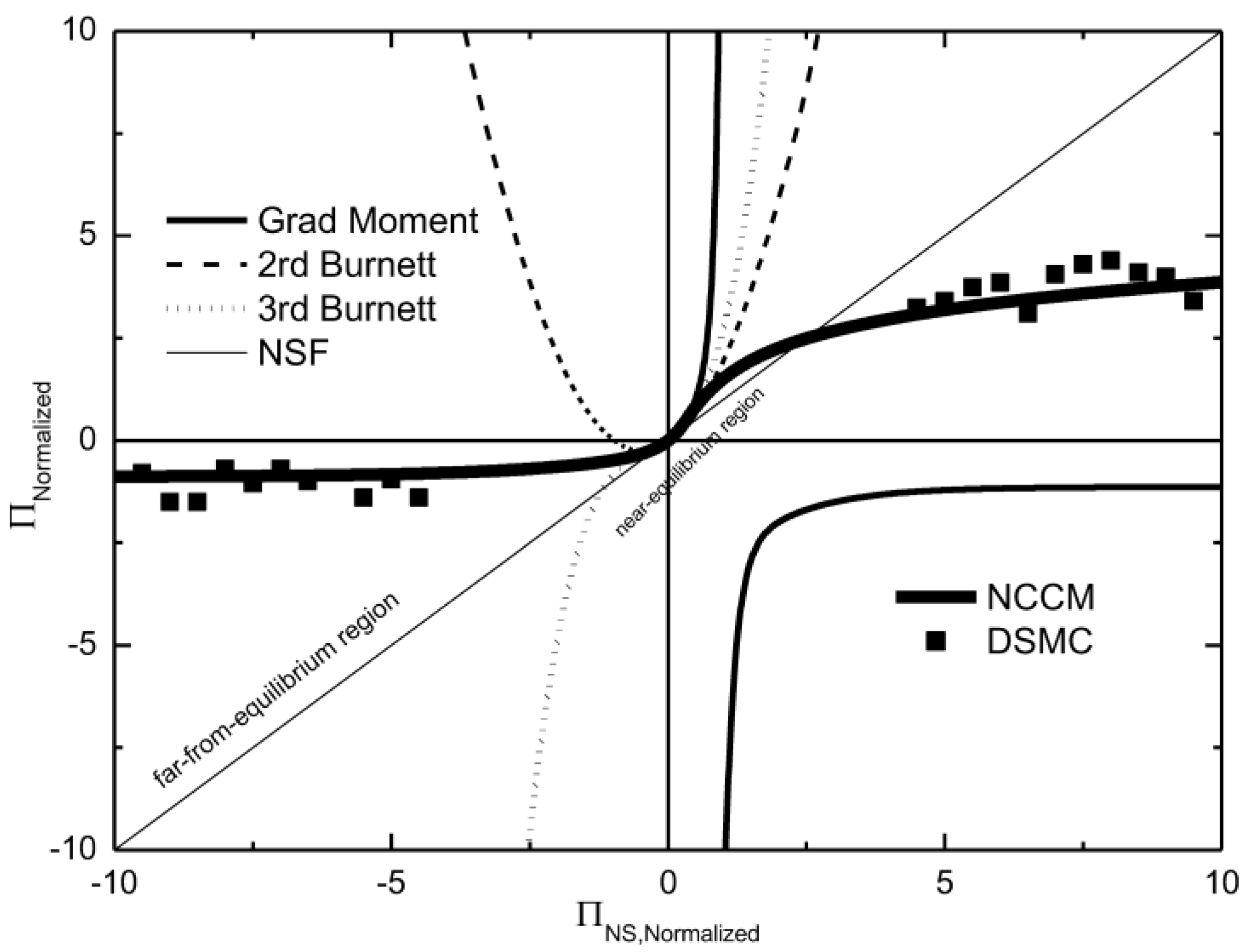
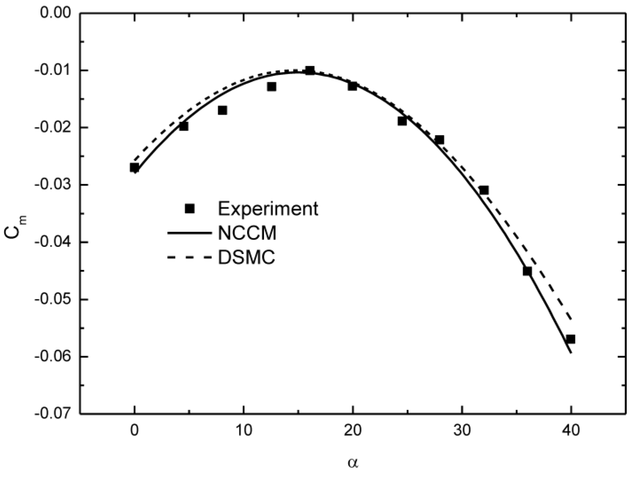
(3)

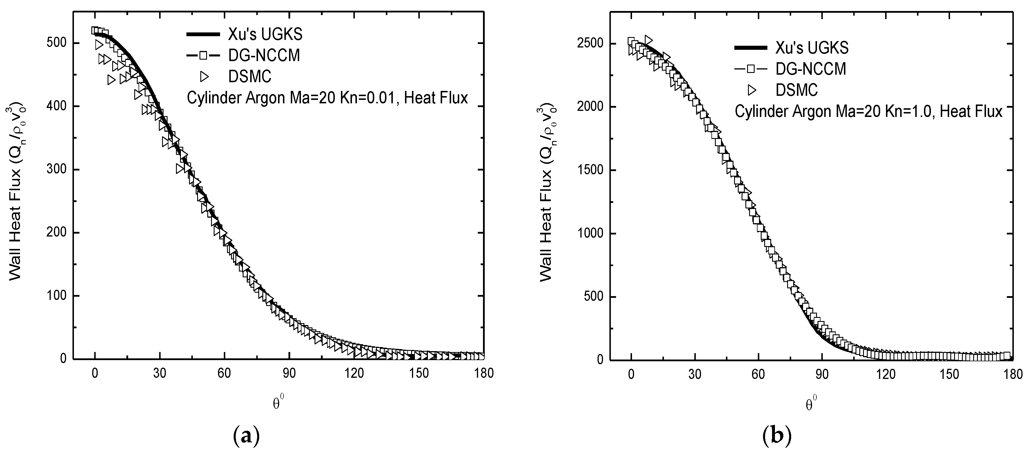
The NCCM has a different nonlinear trend than those of the Burnett equation and the Grad moment method in the far-from-equilibrium region. Note that both the Burnett equation and the Grad moment method cannot be used in far-from-equilibrium states. In contrast, the NCCM shows the opposite trends as those of the Grad moment and Burnett methods. This finding has been validated by the DSMC method, as shown in Figure 1. This feature indicates that the NCCM can be used to describe the gas flow in the far-from-equilibrium state.

4. Results

In the section above, we can see that the NCCM equations approach the NSF equation for near-equilibrium states. In addition, this equation can be validated by the DSMC in far-equilibrium states. For validation, we first provide the verification and validation of the NCCM based on experimental results. Next, we present the test cases of hypersonic gas flows for both a low and a high Kn number. The comparison between the NCCM and the NSF equation at a low Kn number and the comparison between the NCCM and the DSMC method at a high Kn number were both performed in hypersonic gas flows. Furthermore, a comparison among the NCCM results, the DSMC, and the experiment involving three-dimensional (3D) complicated hypersonic vehicles in moment was also conducted. All convergent error is set to be 10⁻⁶.

4.1. Verification and Validation

For verification and validation of the present NCCM equations, the air flows around a NACA 0012 airfoil were first considered. The chord length is regarded as the characteristic length to define Re and the Kn number. To verify grid independence, as shown in

Table 1. Grid independence of Ma = 2.0, Kn = 0.026.

Case	20 × 20	40 × 40	80 × 80	100 × 100
CD	0.4101	0.3951	0.3901	0.3902
CL	9.0 × 10−3	1.23 × 10−4	1.02 × 10−6	1.11 × 10−6

, four sets of meshes are used to calculate the drag coefficient. Next, a set of unstructured triangle meshes, with 100 cells in the airfoil-conforming direction and 100 cells in the wall-normal direction, is implemented in the computational domain. Then, the smallest cell size is less than one percent of chord. Free stream conditions are applied in the outside circle, which has a radius that is 10 times the length of the chord.

Figure 2 presents the dimensionless velocity contours of the NSF equation and the NCCM together with the experimental [27] and DSMC results [8]. All of these results capture the shock wave with a large thickness. The velocity in the after stream of the shockwave is under-predicted by the NSF equation. Both the NCCM and DSMC-IP (Information Preservation) results show good agreement with the experiment, especially in capturing the value of the 0.9 contour at the trailing edge.

4.2. Cavity Flow

Lid-driven cavity flows are studied at high Knudsen numbers. The cavity has a fixed wall temperature T_w = 290 K. The Knudsen number is defined as the ratio of the mean free path to the length of the cavity’s side wall, and the mean free path of gas is evaluated for a hard sphere model. Similar to the previous work [28], the wall velocity is $U_{\infty }=300\mathrm{m}/\mathrm{s}$ for cases at Kn = 0.671 and 6.712. The solutions are compared with the DSMC ones. The computational domain is discretized using a mesh of 100 × 100 cells in physical space. The results of the present study and the DSMC at Kn = 0.671 and 6.712 are presented in Figure 3 and Figure 4, where the temperature contours are shown. Excellent agreements are obtained.

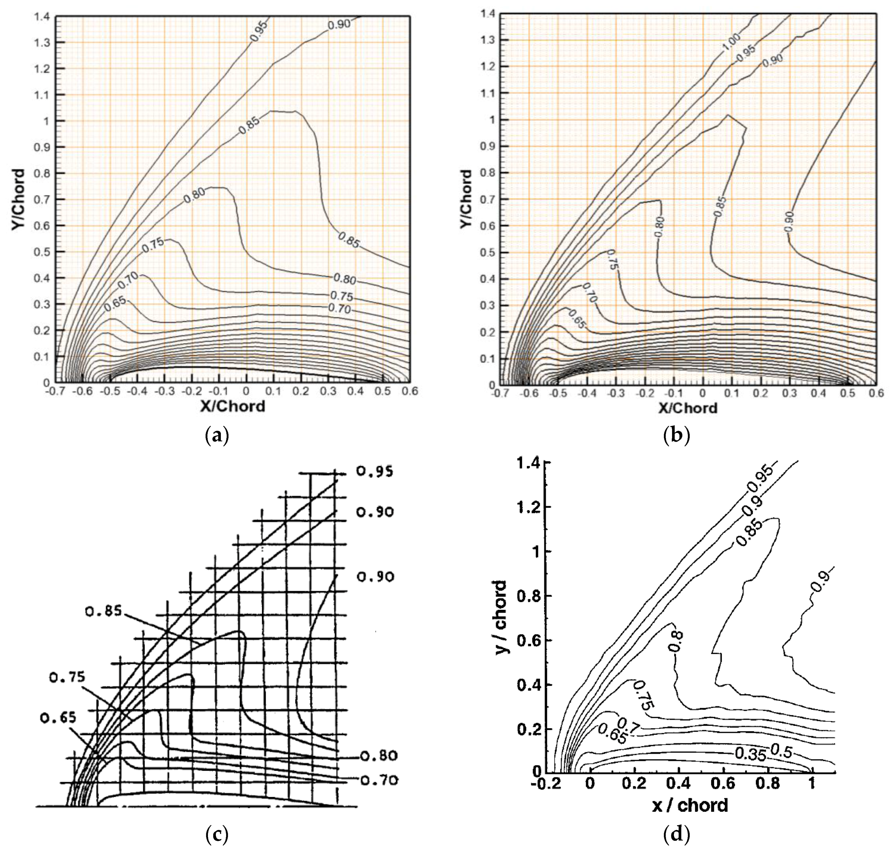
4.3. Hypersonic Gas Flow in a Low Kn Number

In this section, two-dimensional (2D) NCCM is validated for hypersonic gas flows past a circular cylinder. The typical triangular mesh is used in 2D cases, and the outer circular radius that corresponds to a good computational domain is chosen as R_outer = 30 R. The cell size in unstructured mesh is 200 × 120. In other words, there are 200 points on the cylinder surface and 120 points in the radial direction of the computational domain. The linear element (P¹) and the quadratic element (P²) are initially tested for the 2D case; because their numerical results are not distinguishable, the linear element is chosen for all 2D simulations.

The input parameters for the first case are Ma = 5.48, Kn = 0.001, and Pr = 0.607, and the working gas is argon. The contours of Ma number, density, and heat flux are shown in Figure 5; typical distributions around the cylinder are found. Good agreement between the NCCM and the NSF equation was observed. These factors include the position of the shock wave and the contour lines (both in the forebody and the afterbody). This case is for a low Kn number and in the region of near-equilibrium states.

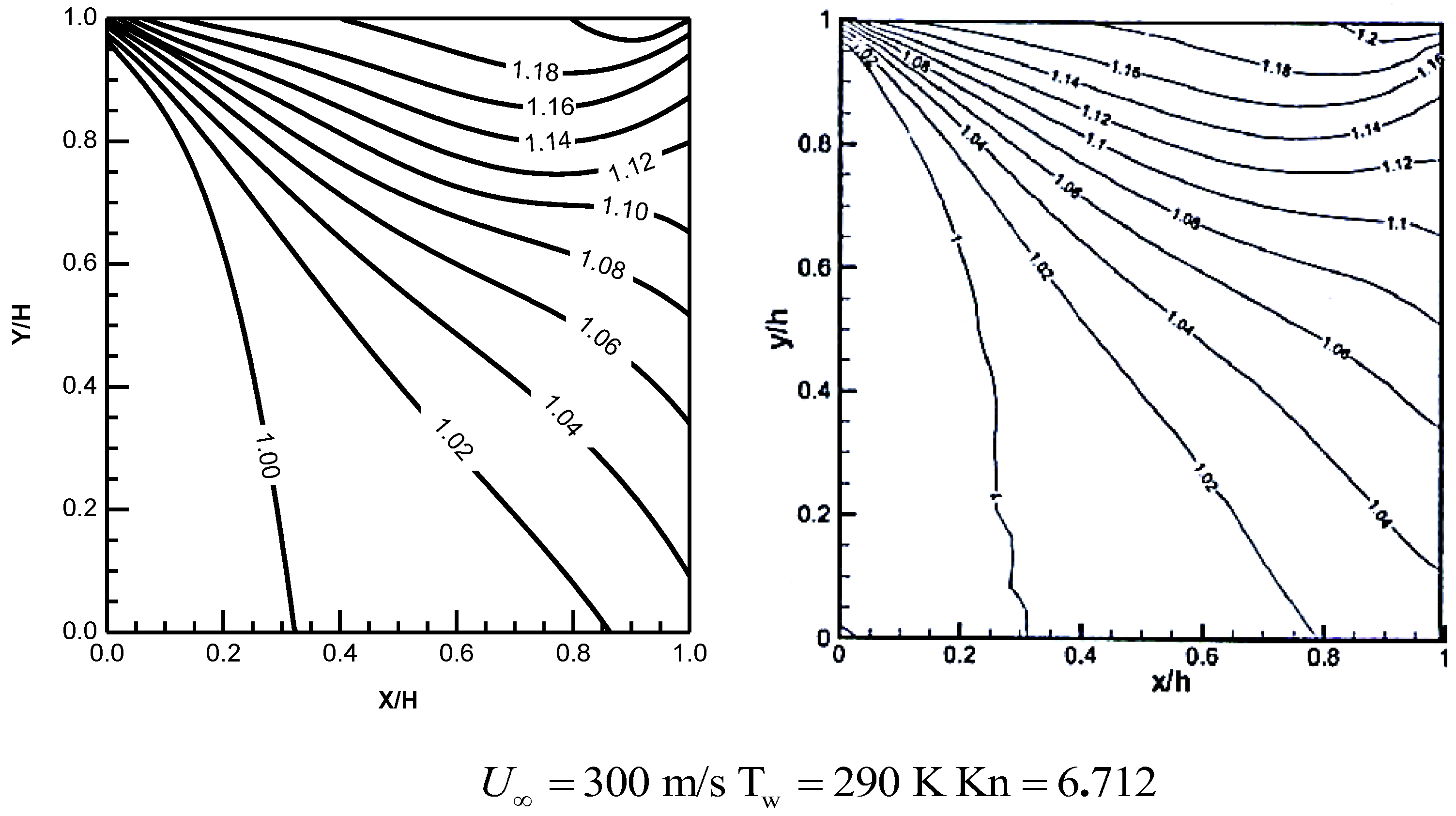
4.4. Hypersonic Gas Flow at a High Kn Number

The input parameters for these two cases are Ma = 20, Kn = 0.01 and Ma = 20, Kn = 1.0. The working gas is argon. The heat fluxes around the solid surface are given in Figure 6. Good agreement of the results of the NCCM and the DSMC and UGKS (Unified gas-kinetic scheme) methods [29] was observed. These two cases are of a high Kn number and in the region of far-equilibrium states.

Furthermore, a 3D NCCM is validated for hypersonic gas flows past 3D complicated hypersonic vehicles as shown in Figure 7 and Figure 8. The typical tetrahedron mesh is used in 3D cases, and the outer circular radius for a good computational domain is chosen as R_outer = 30 R. In this equation, R is the characteristic size of the vehicles. The input parameters for the first case are Ma = 20.0, Kn = 2.531, and Pr = 0.707, and the working gas is air. Good agreement between the results of the NCCM and the DSMC method was observed. This case is of a high Kn number and in the region of far-equilibrium states.

The present authors also validated hypersonic gas flows around a 3D Apollo 6 command module with Ma = 5.0, Kn = 0.5 in the earlier study [4], and good agreement between the results of the NCCM and the DSMC method was observed in this case. Here, we just give the results as can be seen in Figure 9 to prove that the NCCM can solve the problems of far equilibrium. More details can be seen in reference [4].

5. Discussion

The processes for the derivation of the NCCM equations from the Boltzmann equation were given in detail in the present study. The two features implemented in this derivation are discussed in detail. First, the H theorem and positive entropy generation are considered in the irreversible process. In addition, the definition of the distribution function is formal and dynamic. Second, based on the constraint of positive entropy generation, the unified highly nonlinear dissipation model from the nonequilibrium state to the equilibrium state is derived; this model turns into the Rayleigh–Onsager dissipation function near the equilibrium state. Next, the nonlinear coupled constitutive relations of viscous stress and heat flux, which strictly fulfil the second law of thermodynamics, were derived. In addition, coupled with the conservative laws of mass, moment, and energy, a unified scheme for continuum and rarefied gas flow was proposed. A comparison among the Grad moment method, the Burnett equation, and the NCCM was presented. In addition, the differences and relationships between the NCCM equations and the Navier–Stokes–Fourier equations were explained in detail.

For validation, numerical studies of rarefied and continuum gas flows were conducted. These studies include rarefied and/or continuum gas flows around a cylinder and a 3D model of a space shuttle. It was observed that the present results of the NCCM equations were in good agreement with those of the DSMC and UGKS methods in rarefied cases and were in good agreement with those of the Navier–Stokes equations in continuum cases. All these results indicate that the present NCCM equations provide a new approach for developing a unified scheme for solving continuum-rarefied gas flows.

References

1. Shahabi, V.; Baier, T.; Roohi, E.; Hardt, S. Thermally induced gas flows in ratchet channels with diffuse and specular boundaries. Sci. Rep. 2017, 7, 41412. [Google Scholar] [CrossRef] [PubMed]
2. Zhang, P.; Hu, L.; Meegoda, J.N.; Gao, S. Micro/nano-pore network analysis of gas flow in shale matrix. Sci. Rep. 2015, 5, 13501. [Google Scholar] [CrossRef] [PubMed]
3. Zhao, J.; Yao, J.; Zhang, M.; Zhang, L.; Yang, Y.; Sun, H.; An, S.; Li, A. Study of gas flow characteristics in tight porous media with a microscale lattice Boltzmann model. Sci. Rep. 2016, 6, 32393. [Google Scholar] [CrossRef] [PubMed]
4. Xiao, H.; Tang, K. A Unified Framework for Modelling Continuum and Rarefied Gas Flows. Sci. Rep. 2017, 7, 13108. [Google Scholar] [CrossRef] [PubMed]
5. Hadjiconstantinou, N.G. The limits of Navier-Stokes theory and kinetic extensions for describing small-scale gaseous hydrodynamics. Phys. Fluids 2006, 18, 111301. [Google Scholar] [CrossRef]
6. Bird, G.A. Molecular Gas Dynamics and the Direct Simulation of Gas Flows; Claredon: Oxford, UK, 1994; pp. 115–123. [Google Scholar]
7. Bird, G.A. The DSMC Method; Version 1.1.; Claredon: Oxford, UK, 2013; pp. 101–136. [Google Scholar]
8. Fan, J.; Boyd, I.D.; Cai, C.P.; Hennighausen, K.; Candler, G.V. Computation of rarefied gas flows around a NACA 0012 airfoil. AIAA J. 2001, 39, 618–625. [Google Scholar] [CrossRef]
9. Sun, Q.; Boyd, I.D. Flat-plate aerodynamics at very low Reynolds number. J. Fluid Mech. 2004, 502, 199–206. [Google Scholar] [CrossRef]
10. Higuera, F.J.; Succi, S.; Benzi, R. Lattice gas dynamics with enhanced collisions. EPL (Europhys. Lett.) 1989, 9, 345. [Google Scholar] [CrossRef]
11. Benzi, R.; Succi, S.; Vergassola, M. The lattice Boltzmann equation: Theory and applications. Phys. Rep. 1992, 222, 145–197. [Google Scholar] [CrossRef]
12. Montessori, A.; Prestininzi, P.; la Rocca, M.; Succi, S. Lattice Boltzmann approach for complex nonequilibrium flows. Phys. Rev. E 2015, 92, 043308. [Google Scholar] [CrossRef] [PubMed]
13. Nabovati, A.; Sellan, D.P.; Amon, C.H. On the lattice Boltzmann method for phonon transport. J. Comput. Phys. 2011, 230, 5864–5876. [Google Scholar] [CrossRef]
14. He, X.; Chen, S.; Zhang, R. A lattice Boltzmann scheme for incompressible multiphase flow and its application in simulation of Rayleigh–Taylor instability. J. Comput. Phys. 1999, 152, 642–663. [Google Scholar] [CrossRef]
15. Chen, H.; Kandasamy, S.; Orszag, S.; Shock, R.; Succi, S.; Yakhot, V. Extended Boltzmann kinetic equation for turbulent flows. Science 2003, 301, 633–636. [Google Scholar] [CrossRef] [PubMed]
16. Burnett, D. The distribution of molecular velocities and the mean motion in a non-uniform gas. Proc. Lond. Math. Soc. 1936, 2, 382–435. [Google Scholar] [CrossRef]
17. Comeaux, K.A.; Chapman, D.R.; MacCormack, R.W. An analysis of the Burnett equations based on the second law of thermodynamics. In Proceedings of the 33rd AIAA, Aerospace Sciences Meeting and Exhibit, Reno, NV, USA, 12 January 1995. [Google Scholar]
18. Grad, H. On the kinetic theory of rarefied gases. Commun. Pure Appl. Math. 1949, 2, 331–407. [Google Scholar] [CrossRef]
19. Torrilhon, M.; Struchtrup, H. Boundary conditions for regularized 13-moment-equations for micro-channel-flows. J. Comput. Phys. 2008, 227, 1982–2011. [Google Scholar] [CrossRef]
20. Torrilhon, M. Special issues on moment methods in kinetic gas theory. Contin. Mech. Thermodyn. 2009, 21, 341–343. [Google Scholar] [CrossRef]
21. Eu, B.C. Kinetic Theory and Irreversible Thermodynamics; Wiley: New York, NY, USA, 1992. [Google Scholar]
22. Myong, R.S. A generalized hydrodynamic computational model for rarefied and microscale diatomic gas flows. J. Comput. Phys. 2004, 195, 655–676. [Google Scholar] [CrossRef]
23. Myong, R.S. On the high Mach number shock structure singularity caused by overreach of Maxwellian molecules. Phys. Fluids 2014, 26, 056102. [Google Scholar] [CrossRef]
24. Xiao, H.; Shang, Y.H.; Wu, D.; Shi, Y.Y. Nonlinear coupled constitutive relations and its validation for rarefied gas flows. Acta Aeronaut. Astronaut. Sin. 2015, 36, 2091–2104. [Google Scholar]
25. Le, N.T.P.; Xiao, H.; Myong, R.S. A triangular discontinuous Galerkin method for non-Newtonian implicit constitutive models of rarefied and microscale gases. J. Comput. Phys. 2014, 273, 160–184. [Google Scholar] [CrossRef]
26. Xiao, H.; Myong, R.S. Computational simulations of micro scale shock–vortex interaction using a mixed discontinuous Galerkin method. Comput. Fluids 2014, 105, 179–193. [Google Scholar] [CrossRef]
27. Allegre, J.; Raffin, M.; Gottesdient, L. Slip Effect on Supersonic Flow Fields Around NACA 0012 Airfoils, Rarefied Gas Dynamics 15; Boffi, V., Cercigani, C., Eds.; Vieweg + Teubner Verlag: Braunschweig, Germany, 1986; pp. 548–557. [Google Scholar]
28. Zhu, Y.; Zhong, C.; Xu, K. Implicit unified gas-kinetic scheme for steady state solutions in all flow regimes. J. Comput. Phys. 2016, 315, 16–38. [Google Scholar] [CrossRef]
29. Chen, S.Z.; Guo, Z.L.; Xu, K. Simplification of the unified gas kinetic scheme. Phys. Rev. E 2016, 94, 023313. [Google Scholar] [CrossRef] [PubMed]
Figure 1. Comparisons of the normal viscous stress in the nonlinear coupled constitutive method (NCCM) and the Grad, Burnett, and Navier–Stokes–Fourier (NSF) methods.
Entropy 19 00683 g001
Figure 2. Comparison among the NSF, NCCM, Experiment, and direct simulation Monte Carlo (DSMC) velocity fields. (a) NSF; (b) NCCM; (c) Experiment [27]; (d) DSMC-IP [8].
Entropy 19 00683 g002
Figure 3. Comparison among the NCCM (left) and DSMC (right) temperature contours.
Entropy 19 00683 g003
Figure 4. Comparison among the NCCM (left) and DSMC (right) temperature contours.
Entropy 19 00683 g004
Figure 5. The contours of Ma number, density, and Qx (heat flux in the × direction) of High Mach Number gas flow around a Cylinder at Ma = 5.48 and Kn = 0.001. NSF (Top), NCCM (Bottom).
Entropy 19 00683 g005
Figure 6. Normalized Heat Flux around the Solid Surface of High Mach Number gas flow around a Cylinder. (a) Ma = 20, Kn = 0.01; (b) Ma = 20, Kn = 1.0.
Entropy 19 00683 g006
Figure 7. Three-dimensional (3D) configuration for validation.
Entropy 19 00683 g007
Figure 8. Distribution of the Normalized pitch moment at Ma = 20, Kn = 2.531.
Entropy 19 00683 g008
Figure 9. The comparisons of temperature and pressure coefficients on Ma = 5.0, Kn = 0.5.
Entropy 19 00683 g009