Fault Detection for Vibration Signals on Rolling Bearings Based on the Symplectic Entropy Method

Abstract

Bearing vibration response studies are crucial for the condition monitoring of bearings and the quality inspection of rotating machinery systems. However, it is still very difficult to diagnose bearing faults, especially rolling element faults, due to the complex, high-dimensional and nonlinear characteristics of vibration signals as well as the strong background noise. A novel nonlinear analysis method—the symplectic entropy (SymEn) measure—is proposed to analyze the measured signals for fault monitoring of rolling bearings. The core technique of the SymEn approach is the entropy analysis based on the symplectic principal components. The dynamical characteristics of the rolling bearing data are analyzed using the SymEn method. Unlike other techniques consisting of high-dimensional features in the time-domain, frequency-domain and the empirical mode decomposition (EMD)/wavelet-domain, the SymEn approach constructs low-dimensional (i.e., two-dimensional) features based on the SymEn estimate. The vibration signals from our experiments and the Case Western Reserve University Bearing Data Center are applied to verify the effectiveness of the proposed method. Meanwhile, it is found that faulty bearings have a great influence on the other normal bearings. To sum up, the results indicate that the proposed method can be used to detect rolling bearing faults.

1. Introduction

Rolling bearings are basic and key components in rotary machine systems. Any slight fault will lead to abnormal working states of the rotary machine structures, and even affect the normal running of other components. The caused concurrent faults will bring about economical and personnel losses. Rolling bearings with defects have been widely and deeply investigated from the two aspects of mechanism studies and diagnosis analyses, respectively [1,2,3]. Mechanism studies mainly involve dynamic model designs and theoretical analyses of rolling bearings with surface defects (such as pitting or spalling) from the viewpoint of mechanical dynamics theory [4]. Meanwhile, various nonlinear multi-body dynamic models have been proposed, due to Hertzian contact, unbalanced rotor effects, radial internal clearance, raceway spalls and the size of the rolling elements [4,5,6,7]. Diagnosis analyses cover the exploration and development of approaches for the feature extraction and identification for rolling bearing faults from the viewpoint of signal processing or information theory, such as statistical processing, fractal dimension, linear discriminant analysis, cepstrum analysis, time-frequency analysis, supervised learned processing and so on [8,9,10,11,12,13,14,15,16,17,18,19,20]. Few studies however have investigated and extracted the characteristics of the vibration signals on rolling bearings in terms of dynamics theory. For this, this paper tries to introduce the SymEn method to analyze these vibration signals from the point of view of dynamics.

In order to describe the behavior of rolling bearings, the features extracted from vibration signals are the most commonly high-dimensional feature vectors consisting of values in various domains, such as the time domain, frequency domain, EMD/wavelet domain and so on [20,21,22,23,24,25,26,27,28,29,30,31]. Yang et al. constructed 14-dimensional features including three fractal dimensions and 11 time-domain statistical features to evaluate various fault conditions of rolling bearings [20]. For bearing fault detection, Prieto et al. gave a set of 30-dimension statistic features in the time domain for two channels in the beginning [21]. Wu et al. studied 80 original features from multi-scale entropy (MSE), multi-scale permutation entropy (MPE), multi-scale root-mean-square (MSRMS) and multi-band spectrum entropy (MBSE) [22]. Jiang et al. constructed a feature vector consisting of 59 features from the time, frequency and wavelet domains [23]. Ali et al. used empirical mode decomposition and time-domain statistics to extract 50 features [24]. Yang et al. extracted 35 features to identify the condition of a rotor [25]. Wang et al. extracted a set of 22 statistical features from the time, frequency and time-frequency domains [26]. Mbo’o et al. extracted a 10 × 6 feature matrix by using frequency analysis and statistical measures for the diagnosis of bearing damage [27]. Sun et al. applied a weighted wavelet packet entropy (WWPE) method to construct a feature vector of 50 WWPE values for each moving window [28]. Xu et al. applied multiscale base-scale entropy approaches to construct high-dimensional feature vectors (such as 4-dimensional vectors) for fault diagnosis of rolling bearings [29]. Li et al. used 20 features in the time-domain and frequency-domain to reflect the running states of bearings [30]. Yu gave 20-dimensional original features including Shannon entropy, second order statistics, frequency characteristics, wavelet energy, etc. [31]. However, the high-dimensional fault features often contain a great deal of redundant and irrelevant information so that the corresponding classification techniques cause an increase of computational burden and even a decline of the classification accuracy [32]. In order to avoid these problems, one thinks that the reduction dimension of high-dimensional features is a necessary process. In other words, how to get appropriate features becomes a key step for feature recognition. Various reduction dimension techniques have been developed and applied, such as the marginal fisher analysis (MFA) [23], the principal component analysis (PCA) [33], the generalized discriminate analysis (GDA) [34] and so on, but it can be seen that these methods are related to the intrinsic dimensionality of the analyzed data. That is to say, to a great extent, the recognition performance is dependent on the intrinsic dimension value of the data [35,36]. Although it is still a great challenge to choose an optimal value of the intrinsic dimension, the intrinsic dimension of the analyzed data should come from its system. This paper introduces the SymEn method to research the dimensionality and nonlinearity of the vibration signals by reconstructing a Hamilton matrix of the rolling bearing system in symplectic space.

Symplectic space is an even dimensional phase space. In this space, the geometry transform theory is called symplectic geometry. A Hamilton matrix of the system in symplectic space can be equivalent to its original system. Namely, the eigenvalues of the Hamilton matrix contain the dynamical information of the system, such as dimensions. At present, symplectic geometry theory has been mainly studied in nonlinear differential systems [37,38,39]. However, it has also been applied to deal with the time series from complex systems in the reconstructed phase space, such as dimension estimation, nonlinear analysis, symplectic principal component analysis, reduction noise, data prediction and feature extraction [40,41,42,43]. Meanwhile, a SymEn estimate is an entropy measure for complex systems in symplectic geometry space, which can reflect the intrinsic characteristics of the dynamical systems [44].

The rest of this paper is organized as follows: Section 1 introduces the symplectic entropy method as well as the approximate entropy (ApEn), the sample entropy (SampEn), the fuzzy entropy (FuzzyEn), and the radial basis function (RBF) classifier. Section 2 shows our experimental signals and the vibration data sets from the Case Western Reserve University (CWRU) Bearing Data Center. Section 3 analyzes and discusses the dynamical characteristics of our experimental data based on the SymEn method. The effectiveness of the proposed approach is verified by using RBF classifier to diagnose faults in our experiments in comparisons with the ApEn, SampEn and FuzzyEn methods. Then, the SymEn method with RBF classifier is also applied to detect faults in CWRU data. Finally, Section 4 gives the conclusions.

2. Methodology

From the point of view of dynamics theory, a time series, i.e., one-dimensional signal, can reconstructed the system dynamics according to Takens’ embedding theorem. In other words, for a real time series x (x_i, i = 1, …, N), an attractor X_l×m is reconstructed in phase space and also called the trajectory matrix of the dynamical system:

$$\mathit{X}=\left(\begin{array}{c}{X}_1^m\\ X_2^m\\ ⋮\\ X_l^m\end{array}\right)=\left(\begin{array}{cccc}{x}_1& x_2& \cdots & x_m\\ x_2& x_3& \cdots & x_{m+1}\\ ⋮& ⋮& \cdots & ⋮\\ x_l& x_{l+1}& \cdots & x_N\end{array}\right),$$

(1)

where $X_i^m=\left\{x_i,x_{i+1},\cdots ,x_{i+m-1}\right\}$, i∈(1, N − m + 1), represents a point of the system in the phase space. m is the embedding dimension. l = N − m + 1 is the number of points in R^m. The matrix X contains the dynamical information of the system. In order to keep the dynamical characteristics of the matrix X unchanged, this paper introduces the SymEn method due to the measure preserving transformation of symplectic geometry theory. Moreover, the ApEn, SampEn and FuzzyEn methods are also given for comparison.

2.1. Symplectic Entropy (SymEn)

The SymEn method estimates a SymEn measure based on the energy distribution of the attractor X in symplectic space. The SymEn statistic can better describe the properties of the system by using the symplectic transform, even for the nonlinear dynamic systems [44]. The SymEn algorithm is given as follows: first, the attractor X in (1) is mapped into symplectic space. That is, for the attractor X, one can get a Hamilton matrix M of the system in symplectic space [41]:

$$\mathit{M}=\left(\begin{array}{cc}\mathit{A}& 0\\ 0& -{\mathit{A}}^{\mathit{T}}\end{array}\right),$$

(2)

where A = X^TX. M is equivalent to the attractor X.

Second, eigenvalues of the Hamilton matrix M are obtained by a symplectic similar transform. According to symplectic geometry theory, any Hamilton matrix can remain unchanged during a symplectic similar transform [40]. Then, the eigenvalues of the Hamilton matrix M reflect the dynamical characteristics of the system. The symplectic similar transform is a regular transform based on a bilinear antisymmetric nonsingular cross product, called the symplectic cross product [x, y], vectors x and y ∈ R²ⁿ:

$$\left[x,y\right]=\langle x,\mathit{J}y\rangle ,$$

(3)

where <⋅> denotes the inner product, J is the skew-symmetric matrix:

$$\mathit{J}={\mathit{J}}_{2n}=\left[\begin{array}{cc}0& +{\mathit{I}}_n\\ -{\mathit{I}}_n& 0\end{array}\right],$$

(4)

where I_n is a n-dimensional unit matrix.

In symplectic geometry, the Hamilton matrix M can be transformed into an upper Hessenberg matrix B (b_ij = 0, i > j + 1) by a symplectic matrix H:

$${\mathit{H}}^{\mathit{T}}\mathit{M}\mathit{H}=\left(\begin{array}{cc}\mathit{B}& \mathit{R}\\ 0& {\mathit{B}}^{\mathit{T}}\end{array}\right),$$

(5)

where H can also be a Household matrix, i.e.,

$$\mathit{H}=\mathit{H}(k,\omega )=\left(\begin{array}{cc}\mathit{P}& 0\\ 0& \mathit{P}\end{array}\right),$$

(6)

where:

$$\mathit{P}=I_n-\frac{2\varpi {\varpi }^{*}}{{\varpi }^{*}\varpi }$$

$$\varpi ={(0,\cdots ,0;{\omega }_k,\cdots ,{\omega }_n)}^T\ne 0$$

here, P can be obtained from the matrix A [40,42]. For the matrix A, we can get:

$$\mathit{A}=\left(\begin{array}{cccc}{a}_{11}& a_{12}& \cdots & a_{1n}\\ a_{21}& a_{22}& \cdots & a_{2n}\\ ⋮& ⋮& \cdots & ⋮\\ a_{n1}& a_{n2}& \cdots & a_{nn}\end{array}\right)=\left(\begin{array}{cc}{a}_{11}& {\mathit{A}}_{12}^{(1)}\\ {\alpha }_{21}^{(1)}& {\mathit{A}}_{22}^{(1)}\end{array}\right),$$

(7)

If ${\alpha }_{21}^{(1)}\ne 0$, the elementary reflective array P⁽¹⁾ can be calculated as follows:

$$P^{(1)}=I-2{\varpi }^{(1)}{({\varpi }^{(1)})}^T,$$

(8)

where:

$$\{\begin{array}{c}\begin{array}{c}{\varpi }^{(1)}=\frac{1}{{\rho }_1}\left(S^{(1)}-{\alpha }_1{E}^{(1)}\right)\hfill \\ S^{(1)}={\left(a_{11}^{(1)},a_{21}^{(1)},\cdots ,a_{n1}^{(1)}\right)}^T=\left(a_{11},a_{21},\cdots ,a_{n1}\right)\hfill \end{array}\\ \hspace{0.5em}{\alpha }_1={\Vert S^{(1)}\Vert }_2\hfill \\ \hspace{0.5em}{\rho }_1=\Vert S^{(1)}-{\alpha }_1{E}^{(1)}\Vert \hfill \\ E^{(1)}={\left(1,0,\cdots ,0\right)}^{T}n\times 1\hfill \end{array},$$

(9)

Then:

$$P^{(1)}\mathit{A}=\left(\begin{array}{cccc}{\mu }_1& a_{12}^{(2)}& \cdots & a_{1n}^{(2)}\\ 0& a_{22}^{(2)}& \cdots & a_{2n}^{(2)}\\ ⋮& ⋮& \ddots & ⋮\\ 0& a_{n2}^{(2)}& \cdots & a_{nn}^{(2)}\end{array}\right)={\mathit{A}}^{(2)},$$

(10)

Next:

$$S^{(2)}={\left(0,a_{22}^{(2)},\cdots ,a_{n2}^{(2)}\right)}^T,$$

(11)

The matrix P⁽²⁾ can be constructed:

$$P^{(2)}=I-2{\omega }^{(2)}{({\varpi }^{(2)})}^T,$$

(12)

where:

$$\{\begin{array}{c}\hspace{0.5em}{\alpha }_2={\Vert S^{(2)}\Vert }_2\hfill \\ E^{(2)}={\left(0,1,0,\cdots ,0\right)}^{T}n\times 1\hfill \\ \hspace{0.5em}{\rho }_2=\Vert S^{(2)}-{\alpha }_2{E}^{(2)}\Vert \hfill \\ {\varpi }^{(2)}=\frac{1}{{\rho }_2}\left(S^{(2)}-{\alpha }_2{E}^{(2)}\right)\hfill \end{array},$$

(13)

Thus, A⁽²⁾ can be transformed as A⁽³⁾, in which the values of the second column are all zero except the first two elements:

$$P^{(2)}{\mathit{A}}^{(2)}={\mathit{A}}^{(3)}$$

(14)

One can repeat the above steps until A⁽ⁿ⁾ becomes an upper triangle matrix B. The matrix P can be computed:

$$\mathit{P}=P^{(n)}{P}^{(n-1)}\cdots P^{(1)}$$

(15)

The eigenvalues μ = {μ₁, μ₂, …, μ_m} of matrix B are equal to those of matrix A. The eigenvalues μ are sorted in descending order, i.e., μ₁ > μ₂ > … > μ_k >> μ_k+1 ≥ … ≥ μ_m, called the symplectic principal components of matrix A.

The μ values reflect the distribution of the energy of the system in different directions of symplectic space. The probability space of the system can be expressed as:

$$[\mathit{M}\cdot \mathit{P}]=\{\begin{array}{c}\mathit{M}:{\mu }_1,{\mu }_2,\cdots ,{\mu }_m\\ \mathit{P}:p_1,p_2,\cdots ,p_m\end{array},$$

(16)

$$p_i=\frac{{\mu }_i}{{\displaystyle \sum _{i=1}^m{\mu }_i}}$$

(17)

where m is the embedding dimension, $0\le p_i\le 1$, ${\displaystyle {\sum }_{i=1}^m{p}_i}=1$. p_i describes the uncertainty of the entropy in different directions. Then, the SymEn measure can be defined as follows:

$$SymEn=-{\displaystyle \sum _{i=1}^m{p}_i\log (p_i)},$$

(18)

The SymEn statistic calculates the statistical average and measures the degree of uncertainty about the underlying energy probability distribution referring to the Shannon entropy.

2.2. Approximate Entropy (ApEn)

For the ApEn algorithm [45], when the dimension is equal to m, the distance $d_{ij}^m$ between $X_i^m$ and $X_j^m$ in Equation (1) is defined as:

$$d_{ij}^m=d\left[X_i^m-X_j^m\right]=\max \left\{\left|x_{i+k}-x_{j+k}\right|:k\in (0,m-1)\right\},$$

(19)

Then, the similarity between $X_i^m$ and $X_j^m$ can be described by using a measure $C_i^m(i)$, i.e.,

$$C_r^m(i)=\frac{1}{N-m+1}{\displaystyle \sum _{j=1}^{N-m+1}\Theta (d_{ij}^m-r)},$$

(20)

$$r=k\cdot std(x)$$

(21)

where, std(⋅) means the standard deviation. r represents a predetermined tolerance value. k is a constant larger than zero. Θ is the Heaviside function, i.e.,

$$\Theta (z)=\{\begin{array}{c}1ifz\le 0\\ 0ifz>0\end{array},$$

(22)

Next, one can get φ^m(r) as follows:

$${\phi }^m(r)=\frac{1}{N-m+1}{\displaystyle \sum _{i=1}^{N-m+1}\ln C_r^m(i)},$$

(23)

For m + 1, there is:

$$C_r^{m+1}(i)=\frac{1}{N-m}{\displaystyle \sum _{j=1}^{N-m}\Theta (d_{ij}^{m+1}-r)},$$

(24)

$${\phi }^{m+1}(r)=\frac{1}{N-m}{\displaystyle \sum _{i=1}^{N-m}\ln C_r^{m+1}(i)}$$

(25)

Then, for the time series x with the finite length N, the ApEn value can be defined as:

$$ApEn(m,r,N)={\phi }^m(r)-{\phi }^{m+1}(r),$$

(26)

Here, for given N data points, choices of parameter m and r are required in order to calculate reasonable values of ApEn. In applications, m is generally chosen as 2. r ranges from 0.1 to 0.2 std [45]. Besides, ApEn estimate is bias due to self-matches of the ApEn algorithm [46].

2.3. Sample Entropy (SampEn)

The SampEn algorithm does not count self-matches in order to reduce the bias. For the SampEn estimate, the similarity measure $C_i^m(r)$ is defined as follows:

$$C_r^m(i)=\frac{1}{N-m-1}{\displaystyle \sum _{j=1,j\ne i}^{N-m}\Theta (d_{ij}^m-r)},$$

(27)

Here, the analysis length is chosen as the first N − m vectors of length m so that for 1 ≤ i ≤ N − m, $X_i^m$ and $X_i^{m+1}$ are defined. $d_{ij}^m$ is calculated by using Equation (19) with $i\ne j$. Then:

$${\Phi }^m(r)=\frac{1}{N-m}{\displaystyle \sum _{i=1}^{N-m}{C}_r^m(i)},$$

(28)

and for m + 1, there is:

$$C_r^{m+1}(i)=\frac{1}{N-m-1}{\displaystyle \sum _{j=1,j\ne i}^{N-m}\Theta (d_{ij}^{m+1}-r)},$$

(29)

$${\Phi }^{m+1}(r)=\frac{1}{N-m}{\displaystyle \sum _{i=1}^{N-m}{C}_r^{m+1}(i)}$$

(30)

The SampEn can be calculated by using Equations (28) and (30):

$$SampEn(m,r,N)=-\ln \frac{{\Phi }^{m+1}(r)}{{\Phi }^m(r)},$$

(31)

Here, the choices of m and r are the same as those of ApEn algorithm. The SampEn statistic computes the negative logarithm of a probability associated with the time series as a whole but does not employ a template-wise strategy, whereas the ApEn statistic calculates probabilities in a template-wise fashion. In the other hand, the SampEn statistic employs the same Heaviside function to measure the similarity of vectors as the ApEn does. However, the Heaviside function has the characteristics of the discontinuity and hard boundary, which causes problems in the validity and accuracy of the results for the small tolerance r [45,46].

2.4. Fuzzy Entropy (FuzzyEn)

FuzzyEn algorithm employs the fuzzy membership function instead of the Heaviside function to avoid the above issues in the SampEn and ApEn algorithms [47]. Fuzzy membership function has the features of ambiguous boundaries with a real number in the range [0, 1].

For the FuzzyEn estimate, the similarity measure $C_i^m(r)$ is defined as follows:

$$C_r^m(i)=\frac{1}{N-m-1}{\displaystyle \sum _{j=1,j\ne i}^{N-m}{D}_{ij}^m},$$

(32)

where, $D_{ij}^m$ denotes a fuzzy membership function instead of the Heaviside function Θ(⋅) in Equation (22):

$$D_{ij}^m=\exp \left(\frac{-{(d_{ij}^m)}^2}{r^2}\right),$$

(33)

For m + 1:

$$C_r^{m+1}(i)=\frac{1}{N-m-1}{\displaystyle \sum _{j=1,j\ne i}^{N-m}{D}_{ij}^{m+1}},$$

(34)

$$D_{ij}^{m+1}=\exp \left(\frac{-{(d_{ij}^{m+1})}^2}{r^2}\right)$$

(35)

Then, referring to Equations (28), (30) and (31) in the SampEn algorithm, the FuzzyEn measure for finite datasets can be defined:

$$FuzzyEn(m,r,N)=-\ln \frac{{\Phi }^{m+1}(r)}{{\Phi }^m(r)},$$

(36)

The FuzzyEn has two different main characteristics, i.e., continuity and convexity, from the ApEn and the SampEn. Thus, the similarity changes by continuous degrees and self-similarity are the maximum. Moreover, the FuzzyEn statistic is also the negative natural logarithm of the ratio of Φ^m+1 to Φ^m. The FuzzyEn algorithm is similar to the ApEn and SampEn algorithms. The SymEn algorithm is different from the algorithms of the ApEn, SampEn and FuzzyEn although their first steps are all to reconstruct an attractor from a time series. The SymEn values are calculated by a series of preserving-measure transforms in symplectic space but other entropy values are not done. In the practical application, the SymEn method can choose any embedding dimensions, even high dimensions [44], but the others can often only use low dimensions, such as 2 or 3 dimensions [45,46,47]. For the vibration signals of the rolling bearings, this paper studies the effect of the embedding dimension on the SymEn algorithm.

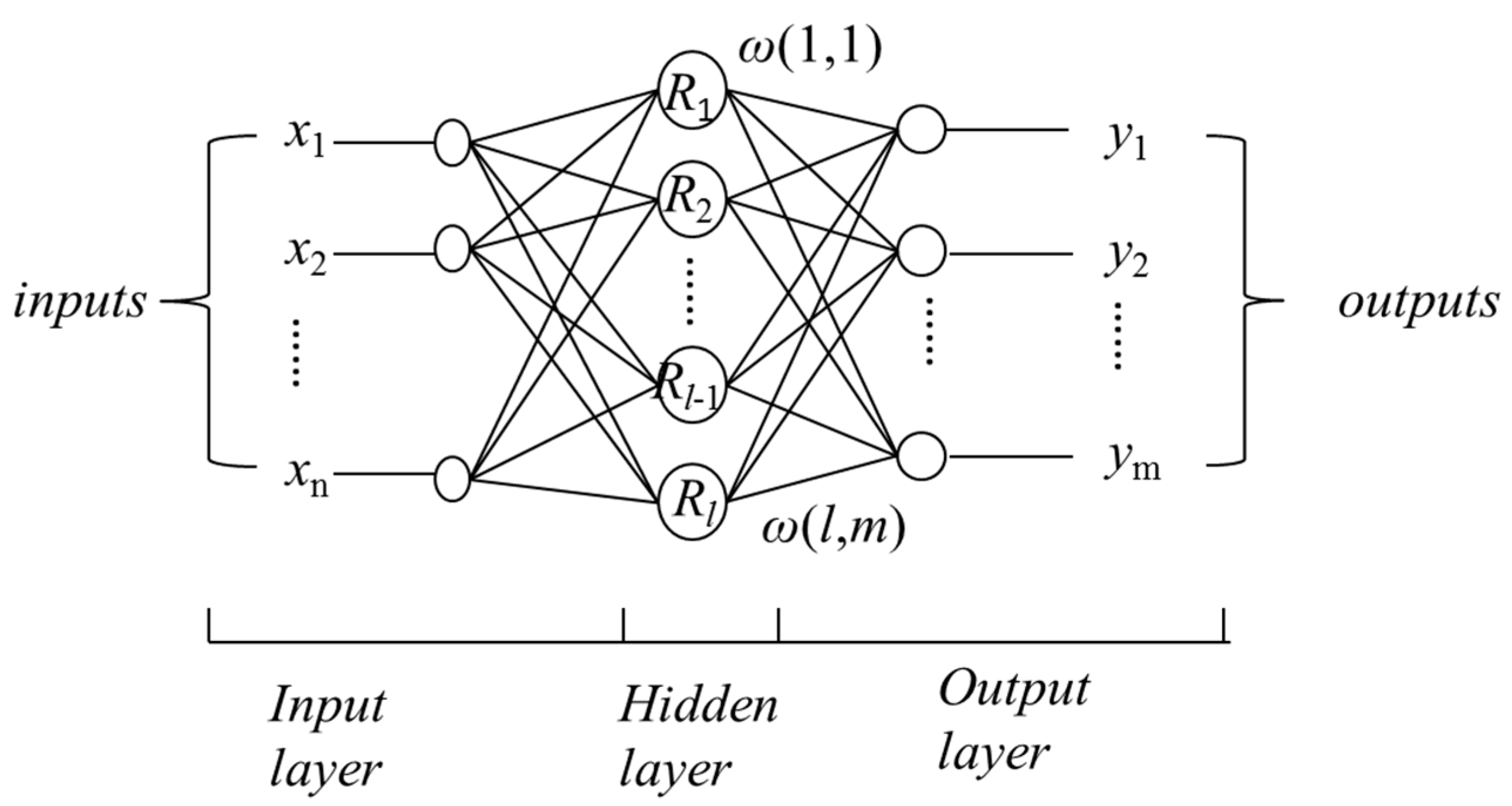
2.5. Radial Basis Function (RBF) Classifier

Classifiers based on RBF have been widely using in different fields for pattern recognition [48]. The RBF classifier includes three totally different layers of an input layer, a hidden layer and an output layer (see Figure 1). The input layer is an interface between input sources and a RBF network. The hidden layer is a high-dimensional nonlinear mapping layer of multiple RBF neurons. The output layer is a layer consisting of linear neurons between the outputs and the hidden layer. Given the input set x_j ∈ Rⁿ, c_i is the center of the i-th radial basis function R_i. y_k is the k-th class output. For the j-th input x_j, the output y_k of the k-th node in the hidden layer is given by the Gaussian radial basis function:

$$y_k(x)={\displaystyle \sum _l{R}_i(x)\times \omega (k,i)}$$

(37)

$$R_i(x)=\exp \left(-\frac{{\Vert x_j-c_i\Vert }^2}{{\sigma }_i^2}\right),i\in [1,l]$$

(38)

where ω(k,i) represents the weight between the i-th node in the hidden layer and the k-th node in the output layer, σ is the dispersion of the Gaussian function. For the algorithm details of the RBF classifier readers may refer to [49].

RBF has global approximation properties and the best approximation performance. Its training processing is also fast and easy. This paper applies the RBF method to classify the four states of rolling bearings.

3. Materials

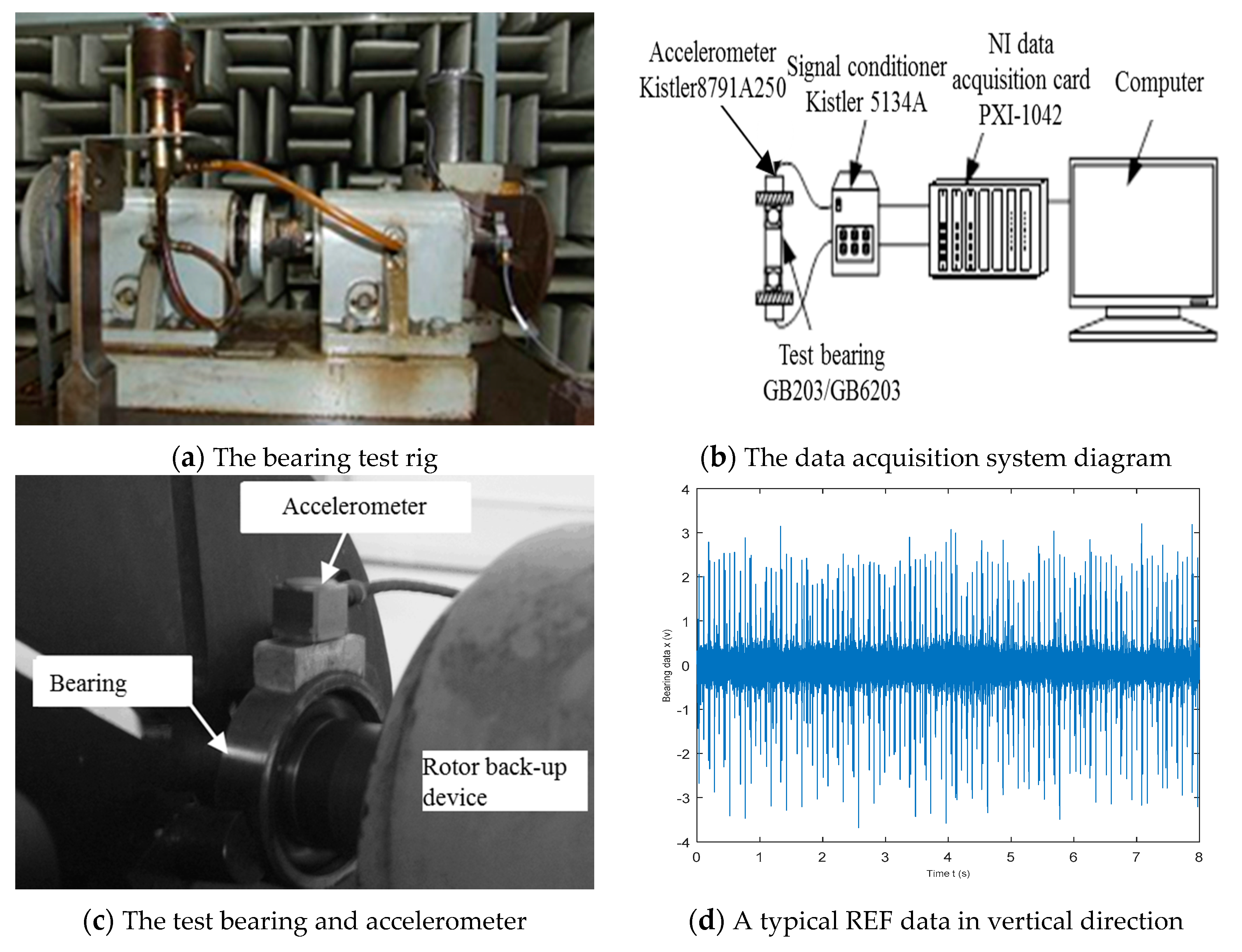
3.1. Case 1: Experimental Vibration Time Series for the Rolling Bearings

In Case 1, two types of the rolling bearings (GB203 and GB6203) are used in order to conveniently analyze them.

Table 1. Parameters of the rolling bearings in Case 1.

Type	Pitch Diameter (mm)	Ball Diameter (mm)	Ball Number	Contact Angle (o)
GB203	28.5	6.747	7	0
GB6203	28.5	6.747	8	0

shows their main parameters. The analyzed data in Case 1 are measured in the running states of the normal condition (NC), outer race fault (ORF), rolling element fault (REF) and the inner race fault (IRF). The ORF, REF and IRF are generated by single pitting on the inner race surface, outer race surface and rolling element surface of the bearings, respectively. The two-channel bearing vibration signals are collected by the data acquisition system with an accelerometer (8791A250, Kistler, Amherst, NY, USA), a signal conditioner (Kistler 5134A), a data acquisition card (PXI-1042, National Instruments, Austin, TX, USA) and a computer on the bearing test rig in the State Key Laboratory of Mechanical System and Vibration (see Figure 2) [50,51]. Channel 1 is the vertical vibration data. Figure 2d shows typical REF vibration data taken in the vertical direction. Channel 2 is the horizontal vibration data. The rotating speed is 720 r/min. The sampling frequency is 25.6 kHz. The total test number of four running states is seven NC tests, three ORF tests, six REF tests and three IRF tests, respectively (see

Table 2. Test times (TT), training set number (TrSN) and testing set number (TeSN) for the data in case 1.

Type	NC TT (TrSN/TeSN)	ORF TT (TrSN/TeSN)	REF TT (TrSN/TeSN)	IRF TT (TrSN/TeSN)
GB203	3 (36/66)	3 (36/66)	3 (36/66)	3 (36/66)
GB6203	4 (48/88)	/	3 (36/66)	/
Overall	7 (84/154)	3 (36/66)	6 (72/132)	3 (36/66)

). The sampling time length of each data is 8 s, i.e., 204,800 points. The length of the analysis data is 6000 points. For training sets, the number of the NC, ORF, REF and IRF data sets is 84, 36, 72 and 36, respectively, in training sets (see Table 2). For testing sets, the number of the NC, ORF, REF and IRF data sets is 154, 66, 132 and 66, respectively (see Table 2).

3.2. Case 2: Standard Reference Data Sets in the CWRU Bearing Database

To further test the utilities of the proposed method, the vibration data sets for 6205-2RS JEM of Svenska Kullager-Fabriken (SKF) deep-groove ball bearings from the website database of the Case Western Reserve University (CWRU) Bearing Data Center (http://csegroups.case.edu/bearingdatacenter/pages/welcome-case-western-reserve-university-bearing-data-center-website) are used [8,23,25,29,30]. These data are acceleration signals in the vertical directions on the housing of drive end (DE) bearing and on the fan end (FE) bearing housing, respectively. The rotor states include the normal condition (NC), three single-point defects (ORF, REF and IRF) at DE as well as NC at FE.

Table 3. The used CWRU bearing data set number (SN) of every classification group for 6205-2RS JEM.

Group Number	Fault Diameter (mm)	NC (SN)	IRF (SN)	REF (SN)	ORF (SN)
1	0.18	100	108	121	133 (6 o’clock)
2	0.18	100	108	121	147 (3 o’clock)
3	0.18	100	108	121	160 (12 o’clock)
4	0.36	100	172	188	200 (6 o’clock)
5	0.53	100	212	225	237 (6 o’clock)
6	0.53	100	212	225	249 (3 o’clock)
7	0.53	100	212	225	261 (12 o’clock)

gives the data set number in seven analyzed data groups with a 12 kHz sampling frequency and the 1730 r/min shaft speed for 6205-2RS JEM of SKF deep-groove ball bearings. The fault depth is 0.11 inches. The fault diameters are 0.18 mm, 0.36 mm and 0.53 mm, respectively. Meanwhile, the ORF position is located at the lowest point (6:00 o’clock), the highest point (12:00 o’clock) and horizontal point (3:00 o’clock), respectively.

4. Results and Analysis

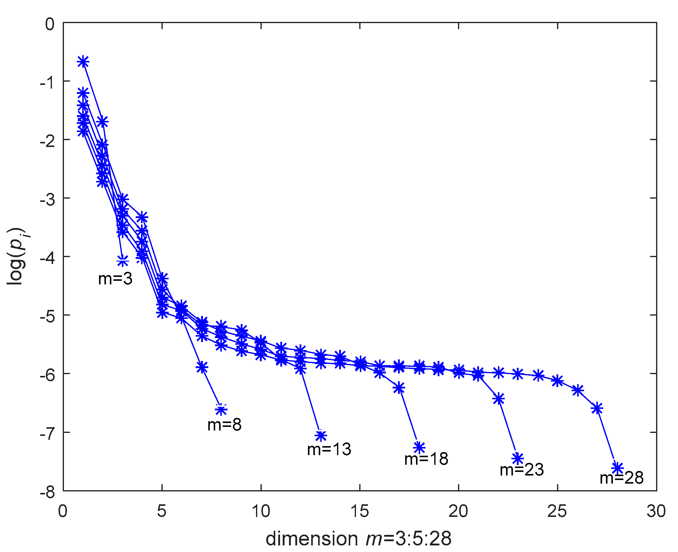
4.1. Dimension Analysis of Vibration Signals for the Rolling Bearing

Dimension estimation is often a basic and important step for the dynamical analysis of vibration time series. Takens’ embedding theorem shows that if the embedding dimension is appropriate, the n-dimension dynamics of a system can be reconstructed from a time series of an observable-measurable system. The reconstructed dynamics properties can reflect the dynamical characteristics of the measured experimental data. Based on Takens’ embedding theorem, the dimension of the bearing time series is estimated by using symplectic geometry referring to our previous study [40]. Figure 3 shows the symplectic geometry spectrums of a typical vibration time series in Figure 2d, which is the logarithm of the energy distribution in Equation (17). The embedding dimension m ranges from 3 to 28. It can be seen that symplectic geometry spectrums gradually decrease with increasing the dimension m, and tend suddenly to flatten at m = 7. Therefore, the embedding dimension is chosen as 7 for the following SymEn analysis on the bearing vibration data.

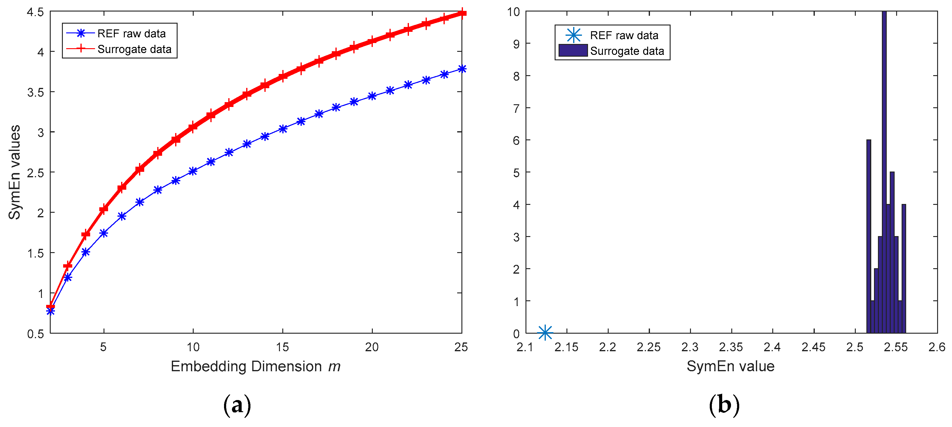
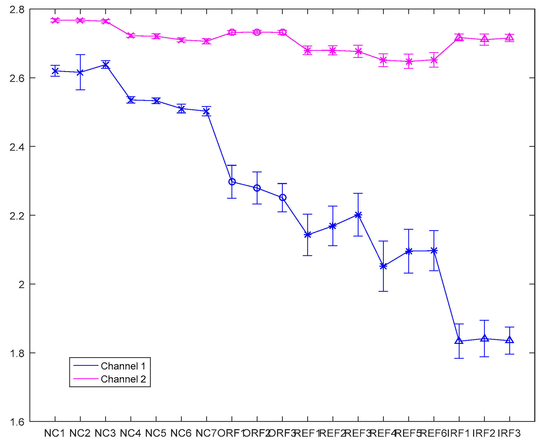
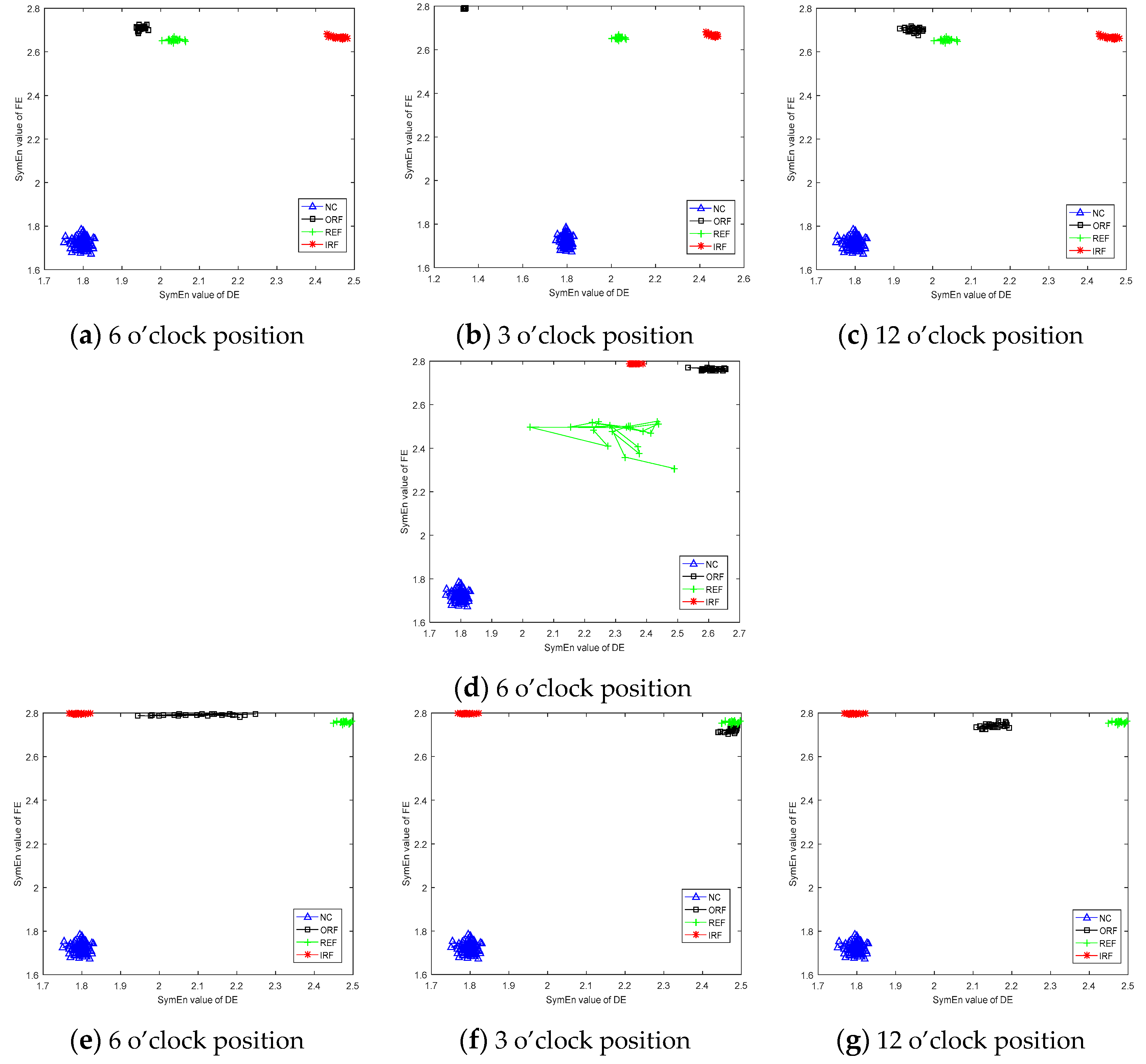
4.2. SymEn Analysis of Vibration Signals for the Rolling Bearing

The SymEn measure reflects the dynamical characteristics of a system. As an entropy estimate, the SymEn value quantifies the lack of information existing in the system by analyzing a time series in symplectic space. Here, the SymEn estimate is used as a test statistic to detect the nonlinear dynamical characteristics of the vibration signals for the rolling bearings. The null hypothesis of a Gaussian linear stochastic process is applied to generate surrogates of the raw vibration signals [52]. The aim of the null hypothesis is to test whether the dynamics of the vibration signals are consistent with a Gaussian linear noise system. According to the null hypothesis, the surrogate data generated from a Gaussian linear noise system contain the same power spectrum and empirical distribution as the raw data by using the iterated amplitude adjusted Fourier transform (IAAFT) algorithm [53]. If there is a significant difference between a test statistic value of the raw data and those of its surrogate data, the null hypothesis is rejected. It indicates that the raw data could be nonlinear. In order to give a judgement in the 95% confidence level, the generated surrogate data are 39 sets. The SymEn values are calculated according to Equation (18). For the rolling bearings, the differences between the SymEn values of the raw vibration data in Figure 2d and those of its surrogate data increases with the increase of the embedding dimension m (see Figure 4a). Figure 4b shows that there is a significant difference between the SymEn value of the raw data and those of its surrogates in m = 7. The null hypothesis can be rejected in the 95% confidence. The raw data does not come from a Gaussian linear stochastic process. The result indicates that the raw data could contain nonlinear dynamical characteristics. Subsequently, this paper furtherly investigates the fault detection of vibration signals by applying the SymEn method.

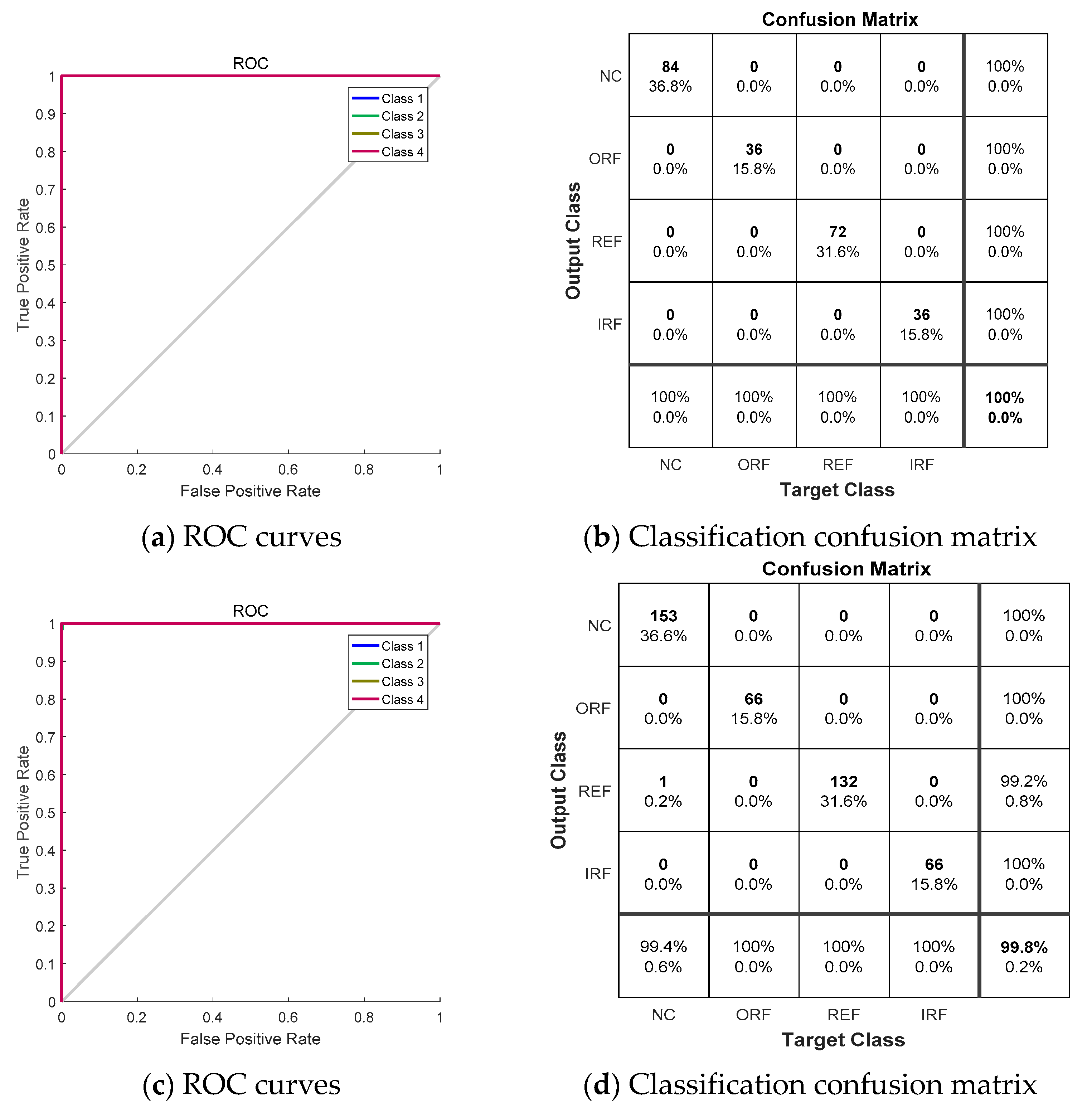
4.3. Fault Detection of Vibration Signals for the Rolling Bearing Based on SymEn

For four running states of rolling bearings in Case 1, the SymEn values of vibration data are calculated with the dimension m = 7 referring to Equation (18). Figure 5 shows the SymEn values of the vibration data for seven NC tests, three ORF tests, six REF tests, three IRF tests in Table 2. We can see that for the same running states, the SymEn values of different tests are very close although the different rolling bearings have some different SymEn values (see Figure 5).

Table 4. SymEn values of vibration signals in four running states.

SymEn	NC Mean ± std	ORF Mean ± std	REF Mean ± std	IRF Mean ± std
Channel 1	2.57 ± 0.06	2.28 ± 0.05	2.13 ± 0.08	1.84 ± 0.05
Channel 2	2.74 ± 0.03	2.73 ± 0.01	2.66 ± 0.02	2.71 ± 0.01

gives the mean and standard deviation of the SymEn values of vibration signals for four running states. The SymEn values of four running states are obviously different. The results indicate that the SymEn measure could reflect the dynamical characteristics of rolling bearings.

Moreover, this paper analyzes the effect of the analysis data length L on the proposed method in order to better detect faults of rolling bearings. The SymEn values of the vibration data in Case 1 are calculated in m = 7 and the data length L ranging from 2000 to 10,000 points. Then, the overall accuracies based on the SymEn values are given by using the radial basis function (RBF) classifier (see

Table 5. Effects of data length L on the SymEn, ApEn, SampEn and FuzzyEn methods for the rolling bearing fault diagnosis.

L	SymEn (%)		ApEn (%)		SampEn (%)		FuzzyEn (%)
	Training	Testing	Training	Testing	Training	Testing	Training	Testing
2000	95.4	93.7	93.2	92.3	90.1	87.9	91.8	90.4
3000	97.3	97.8	94.5	92.4	93.1	91.2	91.3	90.9
4000	100	98.9	97.8	95.5	93.5	92.6	94.7	94.3
5000	100	99	96.2	95.7	93.6	92.7	97.4	95.3
6000	100	99.8	96.9	95.2	93.9	94	99.6	95
7000	100	99.7	97.9	98.3	96.8	95	98.4	96.4
8000	100	99.7	99.4	98.4	94.2	96.4	100	97.7
9000	100	100	99.3	98.5	98	95.1	99.3	96.6
10,000	100	99.6	99.2	99.2	98.5	94.7	99.2	97.6

). For contrast, the ApEn, SampEn and FuzzyEn values are estimated in the dimension m = 2 as well (see Table 5). For the SymEn values, the classification rates increase with the increase of the analysis data length L and tend to a flat in the beginning of the 6000-point data length (see Table 5). For the ApEn, SampEn and FuzzyEn values, the rates tend to a flat in the beginning of the 8000-point data length and are lower than those of the SymEn in the same analysis data length L, so the length of the analysis data can be chosen as 6000 points in this paper. The rates of four running states based on the SymEn estimates are shown in

Table 6. Classification rate (%) of four classes in Case 1 by using SymEn with the RBF classifier.

	NC	ORF	REF	IRF	Overall
Training	100	100	100	100	100
Testing	99.4	100	100	100	99.8

. The above classification features are two-dimension vectors consisting of two SymEn values based on two channels. Comparing with the accuracy rates based on high-dimension features of Case II in the literature [50,51], the results show that the low dimension features based on SymEn can get higher recognition rates. The SymEn estimate could describe the characteristics of different running states for rolling bearings. The SymEn method is superior to other entropy methods. In order to furtherly verify the performance of the proposed method, the receiver operating characteristic (ROC) curves and classification confusion matrix are given in Figure 6. For the training set, the area of ROC curves is 1. For the testing set, the area is 0.9968. The results show that the proposed method can be applied to classify the four states of rolling bearings.

Here, the data in Case 2 from the CWRU database website are analyzed as well. The DE data are considered as the data of channel 1 and the FE data instead of the data of channel 2. The SymEn values are calculated with m = 7 and L = 6000 points. Figure 7 shows the scatter plots based on the SymEn values of DE and FE data for the groups in Table 3. We can see that the SymEn estimates are obviously different for different running states of the DE bearing (see Figure 7). The accuracies are all 100% by RBF classifier for the NC, ORF, REF and IRF (see

Table 7. Classification of the data in Case 2, group number corresponding to Table 3.

Group Number	1	2	3	4	5	6	7
Training (%)	100	100	100	100	100	100	100
Testing (%)	100	100	100	100	100	100	100

). Besides, for the same fault diameter (such as group 1 to 3 and group 5 to 7 in Table 3), the SymEn values are different with the different outer rolling fault positions (see Figure 7a–c,e–f). For the same outer rolling fault position (such as 6 o’clock position), the SymEn values are also different with the different fault diameters (see Figure 7a,d,e). The results indicate that the classification groups of four running states built by the same shaft speed, the same fault diameter and the same outer rolling fault position are help to investigate the dynamic characteristics of rolling bearings. For this, other data of SKF bearings for four different shaft speeds in the CWRU database are grouped into 70 sets like Table 3. The best classification rates are 100%, the worst 84.8%. The analyzed results are not all 100% classification accuracies. Comparing with Case 1, this might be caused by using the vertical direction accelerations at two different points of a horizontal rotation shaft, i.e., the housings of drive end (DE) bearing and the fan end (FE) bearing, respectively. For the normal FE bearing, the SymEn estimates of the data in FE should be very close but are obviously different due to the faults of the DE bearing and vice versa. These results demonstrate that fault bearings have a great impact on other bearings of rotary machine systems, such as fan end bearings or drive end bearings. In other words, even if a bearing is normal, it might be considered as a faulty bearing if another bearing on the same shaft is faulty. Therefore, for fault diagnosis of rolling bearings, the vertical and horizontal accelerations at a test position might better help to detect faults.

Besides, the data in the CWRU database have been widely investigated. In the previous studies, the classification features were often high-dimensional in order to get high accuracy rates [23,25,29,30,50]. By comparison, the low-dimensional features based on SymEn estimate can effectively detect the faults of rolling bearings for the data used in [23,25,29,30,50]. The results indicate that the SymEn estimate could describe the characteristics of different running states for rolling bearings. The performance of the SymEn method is better than those of other high-dimensional approaches.

5. Conclusions

The vibration signals of rolling bearings usually contain non-stationary and nonlinear characteristics. This paper introduces a novel entropy analysis method—the SymEn measure—to investigate the dynamic behavior of rolling bearings. Based on the SymEn analysis, the vibration data of the rolling bearing should be high-dimensional and nonlinear. The dimensions of the data could be chosen as 7 for the data analysis. Based on the SymEn measure, there are significant differences among the dynamic characteristics of the NC, ORF, REF and IRF conditions for the rolling bearings. For the bearing fault detection, the performance of the proposed method is better than those of the ApEn, SampEn, FuzzyEn and other high-dimensional approaches by using the radial basis function classifier. The SymEn measure as a low-dimension feature can provide a higher accuracy rate than the high-dimension features based on time-domain, frequency-domain, wavelet-domain and so on. The results show that the SymEn method better reflects the vibration characteristic information of rolling bearings, and the SymEn method can be applied to diagnose the faults of rolling bearings.

References

1. Shah, D.S.; Patel, V.N. A review of dynamic modeling and fault identifications methods for rolling element bearing. Procedia Technol. 2014, 14, 447–456. [Google Scholar] [CrossRef]
2. Sawalhi, N.; Randall, R.B. Vibration response of spalled rolling element bearings: Observations, simulations and signal processing techniques to track the spall size. Mech. Syst. Signal Process. 2011, 25, 846–870. [Google Scholar] [CrossRef]
3. Henao, H.; Capolino, G.-A.; Fernandez-Cabanas, M.; Filippetti, F.; Bruzzese, C.; Strangas, E.; Pusca, R.; Estima, J.; Riera-Guasp, M.; Hedayati-Kia, S. Trends in fault diagnosis for electrical machines: A review of diagnostic techniques. IEEE Trans. Ind. Electron. Mag. 2014, 8, 31–42. [Google Scholar] [CrossRef]
4. Ahmadi, A.M.; Petersen, D.; Howard, C. A nonlinear dynamic vibration model of defective bearings—The importance of modelling the finite size of rolling elements. Mech. Syst. Signal Process. 2015, 52–53, 309–326. [Google Scholar] [CrossRef]
5. Tadina, M.; Boltežar, M. Improved model of a ball bearing for the simulation of vibration signals due to faults during run-up. J. Sound Vib. 2011, 330, 4287–4301. [Google Scholar] [CrossRef]
6. Kankar, P.K.; Harsha, S.P.; Kumar, P.; Sharma, S.C. Fault diagnosis of a rotor bearing system using response surface method. Eur. J. Mech. A Solids 2009, 28, 841–857. [Google Scholar] [CrossRef]
7. Zheng, J.; Ma, W.; Lin, J.; Ma, L.; Jia, X. Fault diagnosis approach for rotating machinery based on dynamic model and computational intelligence. Measurement 2015, 59, 73–87. [Google Scholar] [CrossRef]
8. Boudiaf, A.; Moussaoui, A.; Dahane, A.; Atoui, I. A comparative study of various methods of bearing faults diagnosis using the Case Western Reserve University Data. J. Fail. Anal. Prev. 2016, 16, 271–284. [Google Scholar] [CrossRef]
9. Immovilli, F.; Bellini, A.; Rubini, R.; Tassoni, C. Diagnosis of bearing faults in induction machines by vibration or current signals: A critical comparison. IEEE Trans. Ind. Appl. 2010, 46, 1350–1359. [Google Scholar] [CrossRef]
10. Borghesani, P.; Pennacchi, P.; Randall, R.B.; Sawalhi, N.; Ricci, R. Application of cepstrum pre-whitening for the diagnosis of bearing faults under variable speed conditions. Mech. Syst. Signal Process. 2013, 36, 370–384. [Google Scholar] [CrossRef]
11. Abboud, D.; Antoni, J.; Eltabach, M.; Sieg-Zieba, S. Angle\time cyclostationarity for the analysis of rolling element bearing vibrations. Measurement 2015, 75, 29–39. [Google Scholar] [CrossRef]
12. Figlus, T.; Stanczyk, M. A method for detecting damage to rolling bearings in toothed gears of processing lines. Metalurgija 2016, 55, 75–78. [Google Scholar]
13. Antoni, J. Cyclic spectral analysis of rolling-element bearing signals: Facts and fictions. Mech. Syst. Signal Process. 2007, 304, 497–529. [Google Scholar] [CrossRef]
14. Straczkiewicz, M.; Czop, P.; Barszcz, T. Supervised and unsupervised learning process in damage classification of rolling element bearings. Diagnostyka 2016, 17, 71–80. [Google Scholar]
15. Tabaszewski, M. Optimization of a nearest neighbors classifier for diagnosis of condition of rolling bearings. Diagnostyka 2014, 15, 37–42. [Google Scholar]
16. Zhang, P.L.; Li, B.; Mi, S.S.; Zhang, Y.T.; Liu, D.S. Bearing fault detection using multi-scale fractal dimensions based on morphological covers. Shock Vib. 2012, 19, 1373–1383. [Google Scholar] [CrossRef]
17. Jin, X.H.; Zhao, M.B.; Chow, T.W.S.; Pecht, M. Motor bearing fault diagnosis using trace ratio linear discriminant analysis. IEEE Trans. Ind. Electron. 2014, 61, 2441–2451. [Google Scholar] [CrossRef]
18. He, Q.B.; Liu, Y.B.; Long, Q.; Wang, J. Time-frequency manifold as a signature for machine health diagnosis. IEEE Trans. Instrum. Meas. 2012, 61, 1218–1230. [Google Scholar] [CrossRef]
19. Fronsini, L.; Harlisca, C.; Szabó, L. Induction machine bearing fault detection by means of statistical processing of the stray flux measurement. IEEE Trans. Ind. Electron. 2015, 62, 1846–1854. [Google Scholar] [CrossRef]
20. Yang, J.; Zhang, Y.; Zhu, Y. Intelligent fault diagnosis of rolling element bearing based on SVMs and fractal dimension. Mech. Syst. Signal Process. 2007, 21, 2012–2014. [Google Scholar] [CrossRef]
21. Prieto, M.D.; Cirrincione, G.; Espionsa, A.G.; Ortega, J.A.; Henao, H. Bearing fault detection by a novel condition-monitoring scheme based on statistical-time features and neural networks. IEEE Trans. Ind. Electron. 2013, 30, 3398–3407. [Google Scholar] [CrossRef]
22. Wu, S.; Wu, C.; Wu, T.; Wang, C. Multi-scale analysis based ball bearing defect diagnostics using mahalanobis distance and support vector machine. Entropy 2013, 15, 416–433. [Google Scholar] [CrossRef]
23. Jiang, L.; Shi, T.; Xuan, J. Fault diagnosis of rolling bearings based on marginal fisher analysis. J. Vib. Control 2014, 20, 470–480. [Google Scholar] [CrossRef]
24. Ali, J.B.; Fnaiech, N.; Saidi, L.; Chebel-Morello, B.; Fnaiech, F. Application of empirical mode decomposition and artificial neural network for automatic bearing fault diagnosis based on vibration signals. Appl. Acoust. 2015, 89, 16–27. [Google Scholar] [CrossRef]
25. Yang, Y.; Zhang, Y.; Zhu, Y. Application of the multi-kernel non-negative matrix factorization on the mechanical fault diagnosis. Adv. Mech. Eng. 2015, 7, 1–11. [Google Scholar] [CrossRef]
26. Wang, X.; Zheng, Y.; Zhao, Z.; Wang, J. Bearing fault diagnosis based on statistical locally linear embedding. Sensors 2015, 15, 16225–16247. [Google Scholar] [CrossRef] [PubMed]
27. Mbo’o, C.P.; Hameyer, K. Fault diagnosis of bearing damage by means of the linear discriminant analysis of stator current feature from the frequency selection. IEEE Trans. Ind. Appl. 2016, 52, 3861–3868. [Google Scholar] [CrossRef]
28. Sun, Y.; Xiong, Z. An optimal weighted wavelet packet entropy method with application to real-time chatter detection. IEEE/ASME Trans. Mechatron. 2016, 21, 2004–2014. [Google Scholar] [CrossRef]
29. Xu, F.; Fang, Y.J.; Kong, Z.M. A fault diagnosis method based on MBSE and PSO-SVM for roller bearings. J. Vib. Eng. Technol. 2016, 4, 383–394. [Google Scholar]
30. Li, W.; Zhang, S.; Rakheja, S. Feature denoising and nearest-farthest distance preserving projection for machine fault diagnosis. IEEE Trans. Ind. Inform. 2016, 12, 393–404. [Google Scholar] [CrossRef]
31. Yu, J. Machinery fault diagnosis using joint global and local/nonlocal discriminant analysis with selective ensemble learning. J. Sound Vib. 2016, 382, 340–356. [Google Scholar] [CrossRef]
32. Gan, M.; Wang, C.; Zhu, C. Multiple-domain manifold for feature extraction in machinery fault diagnosis. Measurement 2015, 75, 76–91. [Google Scholar] [CrossRef]
33. Jung, U.; Koh, B. Wavelet energy-based visualization and classification of high-dimensional signal for bearing fault detection. Knowl. Inf. Syst. 2015, 44, 197–215. [Google Scholar] [CrossRef]
34. Li, J.; Li, S.; Chen, X.; Wang, L. The hybrid KICA-GDA-LSSVM method research on rolling bearing fault feature extraction and classification. Shock Vib. 2015, 2015, 512163. [Google Scholar] [CrossRef]
35. Tenenbaum, J.B.; De Silva, V.; Langford, J.C. A global geometric framework for nonlinear dimensionality reduction. Science 2000, 290, 2319–2323. [Google Scholar] [CrossRef] [PubMed]
36. Roweis, S.; Saul, L. Nonlinear dimensionality reduction by locally linear embedding. Science. 2000, 290, 2323–2326. [Google Scholar] [CrossRef] [PubMed]
37. Zhang, L.; Zhang, L.; Hu, J.F.; Xiong, G.L. Bearing fault diagnosis using a novel classifier ensemble based on lifting wavelet packet transforms and sample entropy. Shock Vib. 2016, 2016, 4805383. [Google Scholar] [CrossRef]
38. Sheng, J.L.; Dong, S.J.; Liu, Z.; Gao, H.W. Fault feature extraction method based on local mean decomposition Shannon entropy and improved kernel principal component analysis model. Adv. Mech. Eng. 2016, 8, 1–8. [Google Scholar] [CrossRef]
39. Zheng, J.D.; Cheng, J.S.; Yang, Y. Multiscale Permutation Entropy Based Rolling Bearing Fault Diagnosis. Shock Vib. 2014, 2014, 154291. [Google Scholar] [CrossRef]
40. Lei, M.; Wang, Z.Z.; Feng, Z.J. A method of embedding dimension estimation based on symplectic geometry. Phys. Lett. A 2002, 303, 179–189. [Google Scholar] [CrossRef]
41. Xie, H.; Dokos, S.; Sivakumar, B.; Mengersen, K. Symplectic geometry spectrum regression for prediction of noisy time series. Phys. Rev. E 2016, 93, 052217. [Google Scholar] [CrossRef] [PubMed]
42. Lei, M.; Meng, G. Symplectic principal component analysis: A new method for time series analysis. Math. Probl. Eng. 2011, 2011, 793429. [Google Scholar] [CrossRef]
43. Lei, M.; Meng, G.A. Noise Reduction Method for Continuous Chaotic Systems Based on Symplectic Geometry. J. Vib. Eng. Technol. 2015, 3, 13–24. [Google Scholar]
44. Lei, M.; Meng, G.; Zhang, W.M.; Wade, J.; Sarkar, N. Symplectic Entropy as a novel measure for complex systems. Entropy 2016, 18, 412–418. [Google Scholar] [CrossRef]
45. Pincus, S.M. Approximate entropy as a measure of system complexity. Proc. Natl. Acad. Sci. USA 1991, 88, 2297–2301. [Google Scholar] [CrossRef] [PubMed]
46. Richman, J.; Moorman, J. Physiological time-series analysis using approximate entropy and sample entropy. Am. J. Physiol. Heart Circ. Physiol. 2000, 278, H2039–H2049. [Google Scholar] [PubMed]
47. Zheng, J.D.; Cheng, J.S.; Yang, Y. A rolling bearing fault diagnosis approach based on LCD and fuzzy entropy. Mech. Mach. Theory 2013, 70, 441–453. [Google Scholar] [CrossRef]
48. Lin, C.-C. Analysis of abnormal Intra-QRS potentials in signal-averaged electrocardiograms using a radial basis function neural network. Sensors 2016, 1580. [Google Scholar] [CrossRef] [PubMed]
49. Haykin, S. Neural Networks: A Comprehensive Foundation, 2nd ed.; Prentice Hall: Upper Saddle River, NJ, USA, 1999. [Google Scholar]
50. Zhou, H.T.; Chen, J.; Dong, G.M.; Wang, R. Detection and diagnosis of bearing faults using shift-invariant dictionary learning and hidden Markov model. Mech. Syst. Signal Process. 2016, 72–73, 65–79. [Google Scholar] [CrossRef]
51. Yuan, H.; Chen, J.; Dong, G. Bearing fault diagnosis based on improved locality-constrained linear coding and adaptive PSO-optimized SVM. Math. Probl. Eng. 2017, 2017, 7257603. [Google Scholar] [CrossRef]
52. Theiler, J.; Eubank, S.; Longtin, A.; Galdrikian, B. Testing for nonlinearity in time series: The method of surrogate data. Phys. D 1992, 58, 77–94. [Google Scholar] [CrossRef]
53. Schreiber, T.; Schmitz, A. Improved surrogate data for nonlinearity tests. Phys. Rev. Lett. 1996, 77, 635–638. [Google Scholar] [CrossRef] [PubMed]
Figure 1. The architecture of the RBF classifier.
Entropy 19 00607 g001
Figure 2. The bearing test rig system and a typical REF data in Case 1.
Entropy 19 00607 g002
Figure 3. The symplectic geometry spectrums of the data in Figure 2d.
Entropy 19 00607 g003
Figure 4. The SymEn analysis of the data in Figure 1b and its surrogate data: (a) SymEn values with the increase of the embedding dimension m = 2:25; (b) SymEn values in m = 7.
Entropy 19 00607 g004
Figure 5. The SymEn values of two-channel vibration data for 7 NC tests, 3 ORF tests, 6 REF tests and 3 IRF tests. The abscissa denotes each test. The ordinate is the SymEn value with mean and standard deviation.
Entropy 19 00607 g005
Figure 6. The performance analysis of the proposed method for the 6000-point data in Case 1: (a,b) for the training sets; (c,d) for the testing sets.
Entropy 19 00607 g006
Figure 7. The scatter plots based on the SymEn values of DE and FE data for the groups in Table 3, outer raceway faults located at 6 o’clock, 3 o’clock and 12 o’clock, respectively: (ac) 0.007-inch fault diameter; (d) 0.014-inch fault diameter; (eg) 0.021-inch fault diameter. The abscissa is the SymEn values of DE data. The ordinate is the SymEn values of FE data.
Entropy 19 00607 g007