Article

Kovacs-Like Memory Effect in Athermal Systems: Linear Response Analysis

Física Teórica, Universidad de Sevilla, Apartado de Correos 1065, E-41080 Sevilla, Spain
*
Author to whom correspondence should be addressed.
Entropy 2017, 19(10), 539; https://doi.org/10.3390/e19100539
Submission received: 19 September 2017 / Revised: 10 October 2017 / Accepted: 11 October 2017 / Published: 13 October 2017
(This article belongs to the Special Issue Thermodynamics and Statistical Mechanics of Small Systems)

Abstract

:
We analyze the emergence of Kovacs-like memory effects in athermal systems within the linear response regime. This is done by starting from both the master equation for the probability distribution and the equations for the physically-relevant moments. The general results are applied to a general class of models with conserved momentum and non-conserved energy. Our theoretical predictions, obtained within the first Sonine approximation, show an excellent agreement with the numerical results. Furthermore, we prove that the observed non-monotonic relaxation is consistent with the monotonic decay of the non-equilibrium entropy.

1. Introduction

The equilibrium state of physical systems is characterized by the value of a few macroscopic variables, for example pressure, volume and temperature in fluids. This characterization of the equilibrium state is complete, in the sense that different samples sharing the same values of the macroscopic variables respond identically to an external perturbation. On the contrary, a system in a nonequilibrium state, even if it is stationary, is not completely characterized by the value of the macroscopic variables: the response to an external perturbation depends also on additional variables or, equivalently, on its entire thermal history. Therefore, it is often said that the response depends on the way the system has been aged.
A pioneering work in the field of memory effects in nonequilibrium systems was carried out by Kovacs [1]. The Kovacs experiment showed that pressure, volume and temperature did not completely characterize the state of a sample of polyvinyl acetate that had been aged for a long time at a certain temperature T 1 . The pressure was fixed during the whole experiment, and the time evolution of the volume was recorded. At a certain time t w , the temperature was suddenly changed to T, for which the equilibrium value of the volume equaled its instantaneous value at t w . Counterintuitively (thinking in equilibrium terms), the volume did not remain constant. Instead, it displayed a hump, passing through a maximum before tending back to its equilibrium (and initial) value.
We look into the Kovacs experiment in a more detailed way in Figure 1. In recent studies of the effect in glassy systems, the relevant physical variable is the energy instead of the volume [2,3,4,5,6,7,8]. The system is equilibrated at a “high” temperature T 0 , and at t = 0 , the temperature is suddenly quenched to a lower temperature T, after which the relaxation function ϕ ( t ) of the energy E is recorded. Specifically, ϕ ( t ) = E ( t ) E e , where E e is the average equilibrium energy at temperature T. Then, a similar procedure is followed, equilibrating the system again at T 0 , but at t = 0 , the temperature is changed to an even lower value T 1 , T 1 < T < T 0 . The system relaxes isothermally at T 1 for a certain time t w , such that E ( t = t w ) equals E e . At this time t w , the temperature is increased to T, but the energy does not remain constant: it displays the behavior that is qualitatively shown by K ( t ) . At first, K ( t ) increases from zero until a maximum is attained for t = t k , and only afterwards, it goes back to zero. Similarly to the relaxation function, we have defined K ( t ) = E ( t ) E e , for t t w . Note that K ( t ) ϕ ( t ) for all times, with the equality being only asymptotically approached in the long time limit.
For molecular (thermal) systems, the equilibrium distribution has the canonical form, and it has been shown that in linear response theory: [6]
K ( t ) = T 0 T 1 T 0 T ϕ ( t ) T T 1 T 0 T ϕ ( t t w ) ,
where the final temperature T and the waiting time t w are related by:
T T 1 T 0 T 1 = ϕ ( t w ) ϕ ( 0 ) .
In linear response, the relaxation function ϕ ( t ) decays monotonically in time because it is proportional to the equilibrium time correlation function (fluctuation-dissipation theorem) E ( 0 ) E ( t ) e E e 2 = i c i exp ( λ i t ) , with c i > 0 and λ i < 0 for all i [9].
The linear response results above make it possible to understand the crux of the observed Kovacs hump in experiments [6]: (i) the inequality 0 K ( t ) ϕ ( t ) , which assures that the hump always has a positive sign (from now on, “normal” behavior), (ii) the existence of only one maximum in the hump and (iii) the increase of the maximum height and the shift of its position to smaller times as t w is decreased. Nevertheless, it must be noted that the experiments, both real [1] and numerical [2,3,4,5,7], are mostly done out of the linear response regime: thus, it seems that the validity of these results extends beyond expectations. In fact, it has been checked in simple models that the linear approximation still gives a fair description of the hump for not-so-small temperature jumps [8].
Very recently, the investigation of Kovacs-like effects in athermal systems has been started. A granular fluid provides a prototypical example of an athermal system, which is intrinsically out-of-equilibrium [10]. A physical mechanism that inputs energy into the system and balances on average the energy loss in collisions, for instance the so-called stochastic thermostat [11], must be considered to reach a nonequilibrium steady state (NESS). Moreover, in general, fluctuations are far more important in granular systems than in molecular systems because of their smallness. The number of particles N, ranging from 10 2 to 10 4 , is large enough to make it possible to apply the methods of statistical mechanics, but definitely much smaller than Avogadro’s number.
The simplest case is that of uniformly-driven granular gases considered in [12,13]. The value of the kinetic energy (granular temperature T g ) at the NESS is controlled by the driving intensity ξ of the stochastic thermostat. Therefore, a Kovacs-like protocol can be implemented in a completely analogous way to the one described above, with the changes T ξ , E T g . One of the main differences found is the emergence of “anomalous” Kovacs behavior for large enough dissipation, when K ( t ) becomes negative and displays a minimum instead of a maximum. It must be stressed that these results have been obtained in the nonlinear regime, that is for driving jumps ξ 0 ξ , ξ 0 ξ 1 that are not small.
More recently, Kovacs-like behavior has been observed in other, more complex, athermal systems. This is the case of disordered mechanical systems [14] and also of active matter [15]. In the latter, a “giant” Kovacs hump has been reported, in the sense that the numerically observed maximum is much larger than the one predicted by the extrapolation of the linear approximation expression (1) to the considered protocol. Moreover, an alternative derivation of (1) has been provided in the supplemental material of [15]. This derivation holds for athermal systems, since it does not make use of either the explicit form of the probability distribution or the relationship between response functions and time correlations at the steady state, but is restricted to discrete-time dynamics at the macroscopic (average) level of description.
The objectives of our paper are two-fold. Firstly, we put forward a rigorous and general derivation of the linear response expression for the Kovacs hump for systems with a realistic continuous time dynamics. This is done at both the mesoscopic and macroscopic levels of description, starting from the master equation for the probability distribution and from the hierarchy of equations for the moments, respectively. Our proof is also valid for athermal systems, since no hypothesis is needed with regard to the form of either the stationary probability distribution or the fluctuation-dissipation relation. Secondly, we apply our results to a simple class of dissipative models that mimic the shear component of a granular fluid, recently introduced [16,17,18]. Therein, we obtain explicit expressions for the Kovacs hump within the first Sonine approximation and compare the theoretical predictions with numerical results. We also discuss the compatibility of the non-monotonic behavior displayed by the granular temperature in the Kovacs experiment and the monotonic approach to the NESS of the nonequilibrium entropy or H-functional [19,20,21].

2. Linear Theory for Kovacs-Like Memory Effects

2.1. General Markovian Dynamics

Here, we consider a general system, whose state is completely characterized by a vector x with M components, x = { x 1 , x 2 , , x M } . For example, in a one-dimensional Ising chain of N spins, x i = σ i = ± 1 , and M = N ; for a gas comprising N particles with positions r i and velocities v i , M = 6 N , and x = { r 1 , v 1 , , r N , v N } . As is customary and for the sake of simplicity, from now on, we use a notation suitable for systems in which the states can be labeled with a discrete index α , 1 α Ω . For example, this is the case of the Ising system above, where Ω = 2 N . The generalization for a continuous index is straightforward, by changing sums into integrals and the Kronecker delta by the Dirac delta [9].
At the mesoscopic level of description, we assume that x is a Markov process, and its dynamics is governed by a master equation for the probabilities P ( x α , t ) ,
t P ( x α , t ) = α ˜ W ( x α | x α ˜ ; ξ ) P ( x α ˜ , t ) W ( x α ˜ | x α ; ξ ) P ( x α , t ) ,
where W ( x α | x α ˜ ; ξ ) are the transition rates from state x α ˜ to state x α , and our notation explicitly marks their dependence on some control parameter ξ . Equation (3) can be formally written as:
t | P ( t ) = W ( ξ ) | P ( t ) ,
where | P ( t ) is a vector (column matrix) whose components are the probabilities P ( x α , t ) and W ( ξ ) is the linear operator (square matrix) that generates the dynamical evolution of | P ( t ) ,
W ( x α | x α ˜ ; ξ ) = W ( x α | x α ˜ ; ξ ) δ α , α ˜ α W ( x α | x α ; ξ ) .
Let us assume that the Markovian dynamics is ergodic (or irreducible [9]), that is all the states are dynamically connected through a chain of transitions with non-zero probability. Therefore, there is a unique steady solution of the master equation | P s ( ξ ) , which verifies:
W ( ξ ) | P s ( ξ ) = 0 ,
and depends on the parameter ξ controlling the system dynamics. Note that ergodicity does not imply detailed balance, so we can have non-zero currents in the steady state. In general, this means that the system approaches an NESS in the long time limit, not an equilibrium state.
Now, we consider the system evolving from a certain initial state at time t 0 , characterized by the distribution | P ( t 0 ) . The formal solution of the master equation can be written as:
| P ( t ) P s ( ξ ) = e ( t t 0 ) W ( ξ ) | P ( t 0 ) P s ( ξ ) .
This is the starting point for our derivation of the expression for the Kovacs effect in the linear response approximation, which is carried out in the next section.
The time evolution of any physical property Y is obtained right away. Let us denote the value of Y for a given configuration x by Y ( x ) : its expected or average value is given by :
Y ( t ) = α Y ( x α ) P ( x α , t ) = Y | P ( t ) ,
where | Y is a ket whose components are Y ( x α ) , and Y | its corresponding bra (row matrix with the same components. Note that we are assuming that Y is a real quantity for all the configurations. By substituting (7) into (8), it is obtained that:
Δ Y ( t ; ξ ) Y ( t ) Y s ( ξ ) = Y | e ( t t 0 ) W ( ξ ) | P ( t 0 ) P s ( ξ ) ,
in which Y s ( ξ ) is the average value at the steady state of the system corresponding to ξ .
Now, we investigate the relaxation of the system from the steady state for ξ 0 = ξ + Δ ξ to the steady state for ξ . We do so in linear response, that is Δ ξ is considered to be small, and we neglect all terms beyond those linear in Δ ξ . Thus, at t = 0 we have that the probability distribution is:
| P ( t = 0 ) = | P s ( ξ + Δ ξ ) = | P s ( ξ ) + Δ ξ | d P s ( ξ ) d ξ + O ( Δ ξ ) 2 .
Substitution of (10) into (9) yields the formal expression for the relaxation of Y in linear response,
Δ Y ( t ; ξ ) = Δ ξ Y | e ( t t 0 ) W ( ξ ) | d P s ( ξ ) d ξ .
In order to have an order of unity function, one may define a normalized relaxation function:
ϕ Y ( t ; ξ ) lim Δ ξ 0 Δ Y ( t ; ξ ) Δ ξ = Y | e ( t t 0 ) W ( ξ ) | d P s ( ξ ) d ξ .
Sometimes, the relaxation function is further normalized by considering ϕ Y ( t ) / ϕ Y ( t = t 0 ) (see for instance [6,22]), but such a multiplying factor is clearly not physically relevant and will not be introduced here.

2.2. The Kovacs Protocol: Linear Response Analysis from the Master Equation

Here, it is a Kovacs-like protocol that we introduce, by considering that the parameter ξ controlling the dynamics is changed in the following stepwise manner:
ξ ( t ) = ξ 0 , < t < 0 , ξ 1 , 0 < t < t w , ξ , t > t w .
Therefore, since ξ 0 is kept for an infinite time, at t = 0 , the system is prepared in the corresponding steady state, P ( t = 0 ) = P s ( ξ 0 ) . Our idea is to consider that the jumps ξ 1 ξ 0 and ξ ξ 1 are small, in the sense that all expressions can be linearized in the magnitude of these jumps. Note that this protocol is completely analogous to the Kovacs protocol described in the Introduction (see Figure 1), but with ξ playing the role of the temperature.
We start by analyzing the relaxation in the first time window, 0 < t < t w . Therein, we apply (7) with the substitutions t 0 0 and ξ ξ 1 , that is,
| P ( t ) P s ( ξ 1 ) = e t W ( ξ 1 ) | P s ( ξ 0 ) P s ( ξ 1 ) , 0 t t w .
The final distribution function, at t = t w , is the initial condition for the next stage, t > t w , in which the system relaxes towards the steady state corresponding to ξ . Making use again of (7) with t 0 t w ,
| P ( t ) P s ( ξ ) = e ( t t w ) W ( ξ ) | P ( t w ) P s ( ξ ) = e ( t t w ) W ( ξ ) e t w W ( ξ 1 ) | P s ( ξ 0 ) P s ( ξ 1 ) + | P s ( ξ 1 ) P s ( ξ ) , t t w .
It must be stressed that the above expressions, Equations (14) and (15), are exact, and no approximation has been made.
The linear response approximation is introduced now: we assume that both jumps ξ 0 ξ 1 and ξ ξ 1 are small, so we can expand both | P s ( ξ 0 ) P s ( ξ 1 ) and | P s ( ξ 1 ) P s ( ξ ) , similarly to what was done in Equation (10). Namely,
| P s ( ξ 0 ) P s ( ξ 1 ) = ( ξ 0 ξ 1 ) | d P s ( ξ ) d ξ + O ( ξ 0 ξ 1 ) 2 ,
| P s ( ξ 1 ) P s ( ξ ) = ( ξ 1 ξ ) | d P s ( ξ ) d ξ + O ( ξ 1 ξ ) 2 .
Note that in both (16a) and (16b), the derivatives are evaluated at ξ ; the difference introduced by evaluating them at either ξ 1 or ξ 0 is second order in the deviations. Then,
| P ( t ) P s ( ξ ) = ( ξ 0 ξ 1 ) e ( t t w ) W ( ξ ) e t w W ( ξ 1 ) | d P s ( ξ ) d ξ + ( ξ 1 ξ ) e ( t t w ) W ( ξ ) | d P s ( ξ ) d ξ .
This equation can be further simplified: since the two terms on its rhs are first order in the jumps, we can substitute W ( ξ 1 ) with W ( ξ ) , with the result:
| P ( t ) P s ( ξ ) = ( ξ 0 ξ 1 ) e t W ( ξ ) | d P s ( ξ ) d ξ ( ξ ξ 1 ) e ( t t w ) W ( ξ ) | d P s ( ξ ) d ξ .
This is the superposition of two responses: the first term on the rhs gives the relaxation from ξ 0 to ξ 1 , which starts at t = 0 , whereas the second term stands for the relaxation from ξ 1 to ξ , which starts at t = t w . We have chosen to write ( ξ ξ 1 ) in the second term because ξ > ξ 1 in the Kovacs protocol.
The same structure in Equation (18) is transferred to the average value. Taking into account Equation (9):
Δ Y ( t ) = ( ξ 0 ξ 1 ) Y | e t W ( ξ ) | d P s ( ξ ) d ξ ( ξ ξ 1 ) Y | e ( t t w ) W ( ξ ) | d P s ( ξ ) d ξ , t t w ,
in which we recognize the relaxation function in linear response, defined in Equation (12). We can also normalize the response in this experiment, by defining a function K ( t ) as follows,
K Y ( t ) lim ξ 0 ξ Δ Y ( t ) ξ 0 ξ = ξ 0 ξ 1 ξ 0 ξ ϕ Y ( t ) ξ ξ 1 ξ 0 ξ ϕ Y ( t t w ) .
It is understood that, as ξ 0 ξ 0 , both prefactors ξ 0 ξ 1 ξ 0 ξ and ξ ξ 1 ξ 0 ξ are kept of the order of unity.
A few comments on Equation (20) are in order. Hitherto, no restriction has been imposed on the state of the system at t = t w ; therefore, (20) is valid for arbitrary ( ξ 0 , ξ 1 , ξ ) , provided that the jumps are small enough and the ratio of the jumps is of the order of unity. The function K ( t ) corresponds to a Kovacs-like experiment when ξ is chosen as a function of t w in such a way that Y ( t w ) = Y s ( ξ ) or K Y ( t w ) = 0 , that is,
ξ ξ 1 ξ 0 ξ 1 = ϕ Y ( t w ) ϕ Y ( 0 ) .
Alternatively, one may consider that (21) defines t w as a function of ξ .
The complete analogy between Equations (20) and (21) and Equations (1) and (2) is apparent. Nevertheless, we have made use neither of the explicit form of the steady state distribution (in general non-canonical), nor of the relation between response functions and time correlation functions (fluctuation-dissipation relation), which were necessary in [6] to demonstrate Equation (1). Therefore, the proof developed here is more general, being valid for any steady state, equilibrium or nonequilibrium, and thus, it specifically holds in athermal systems. Furthermore, it must be noted that it can be easily extended to the Fokker–Planck, or the equivalent Langevin, equation.

2.3. Linear Response from the Equations for the Moments

In this section, we do not start from the equation for the probability distribution, but from the equations for the relevant physical properties of the considered system. For example, one may think of the hydrodynamic equations for a fluid or the law of mass action equations for chemical reactions. Of course, these equations can be derived in a certain “macroscopic” approximation [9], which typically involves neglecting fluctuations, from the equation for the probability distribution by taking moments, but this is not our approach here. Anyhow, we borrow this term to call our starting point “equations for the moments”.
We denote the relevant moments by z i , i = 1 , , J , where J is the number of relevant moments. The equations for the moments have the general form:
d d t z i = f i ( z 1 , , z J ; ξ ) ,
where f i are continuous, in general nonlinear, functions of the moments. This is a key difference between moment equations and the master (or Fokker–Planck) equation, since the latter is always linear in the probability distribution. Therefore, unlike the master equation, Equation (22) cannot be formally solved for arbitrary initial conditions. This notwithstanding, in the linear response approximation, we show here that a procedure similar to the one carried out in the previous section leads to the same expression for the Kovacs hump.
We assume that there is only one steady solution of Equation (22) that is globally stable, at which the corresponding values of the moments are z i s ( ξ ) . Linearization of the dynamical system around the steady state gives:
d d t | Δ z ( t ) = M ( ξ ) | Δ z ( t ) , | Δ z ( t ) | z ( t ) z s ( ξ ) .
We are using a notation completely similar to that in the previous section: | z is a vector, represented by a column matrix with components z i , and M ( ξ ) is a linear operator, represented by a square matrix with elements:
M i j ( ξ ) = z j f i | z = | z s ( ξ ) .
Note that the dimensions of these matrices are much smaller than those for the master equation, since J is of the order of unity and does not diverge in the thermodynamic limit. In general, M i j M j i , and the operator M is not Hermitian. However, we do not need M to be Hermitian to solve the linearized system in a formal way, as shown below.
Analogously to what was done for the master equation, the formal solution of Equation (23) is:
| Δ z ( t ) = e ( t t 0 ) M ( ξ ) | Δ z ( t 0 ) .
In particular, if the initial condition is chosen to correspond to the steady state for ξ 0 = ξ + Δ ξ , one has:
| Δ z ( t ) = Δ ξ e ( t t 0 ) M ( ξ ) | d z s ( ξ ) d ξ .
The response for any of the relevant moments can be extracted by projecting the above result onto the “natural” basis | u i , whose components are u i j = δ i j . Then, the normalized linear response function for z i can be defined by:
ϕ z i ( t ) = lim Δ ξ 0 u i | Δ z ( t ) Δ ξ = u i | e ( t t 0 ) M ( ξ ) | d z s ( ξ ) d ξ .
Note the utter formal analogy of Expression (27) with Equation (12), which was obtained from the master equation. The proof of the expression for the Kovacs hump follows exactly the same line of reasoning, and the result is exactly that in Equations (20) and (21); thus, it is not repeated here.

3. A Lattice Model with Conserved Momentum and Non-Conserved Energy

3.1. Definition of the Model: Kinetic Description

Here, we briefly put forward a class of models for the shear component of the velocity in a granular gas, focusing on the features that are needed for the discussion of memory effects. A more complete description of the model, including its physical motivation, can be found in [16,17,18,23].
The system is defined on a 1d lattice: there is a particle with velocity v l at each site l. The system configuration is thus given by v { v 1 , . . . , v N } . The dynamics proceeds through inelastic nearest-neighbor binary collisions: each pair ( l , l + 1 ) collides inelastically with a characteristic rate proportional to | v l v l + 1 | β , with β 0 . For β = 0 , nearest-neighbor particles collide independently of their relative velocity (the so-called Maxwell-molecule model [24]), whereas for β = 1 and β = 2 , we have a collision rate analogous to that of hard spheres and very hard spheres, respectively [10,25]. The pre-collisional velocities are transformed into the post-collisional ones by the operator b ^ l ,
b ^ l v l = v l 1 + α 2 v l v l + 1 ,
b ^ l v l + 1 = v l + 1 + 1 + α 2 v l v l + 1 ,
where 0 < α 1 is the normal restitution coefficient. Momentum is always conserved in collisions, ( b ^ l 1 ) ( v l + v l + 1 ) = 0 , but energy is not; in fact, ( b ^ l 1 ) ( v l 2 + v l + 1 2 ) = ( α 2 1 ) ( v l v l + 1 ) 2 / 2 0 , with equality holding only in the elastic limit α = 1 .
In order to have a steady state, a mechanism that injects energy into the system, and thus compensates on average the energy loss in collisions, must be introduced. For the sake of simplicity, we consider here that the system is “heated” by a white noise force, that is the so-called stochastic thermostat [11,26]. The velocity change introduced by the stochastic forcing is:
τ v i ( τ ) noise = ξ i ( τ ) 1 N j = 1 N ξ j ( τ ) ,
and ξ i ( τ ) are Gaussian white noises of amplitude χ :
ξ i ( τ ) noise = 0 , ξ i ( τ ) ξ j ( τ ) noise = χ δ i j δ ( τ τ ) ,
for i , j = 1 , , N . This version of the stochastic thermostat conserves total momentum, which is needed to assure the existence of a well-defined steady state [27,28].
We do not write here the master-Fokker–Planck equation for the N-particle P N ( v , τ ) probability density of finding the system in state v at time τ . Instead, we directly write the “kinetic” equation for the one-particle distribution function, namely P 1 ( v ; l , τ ) = d v P N ( v , τ ) δ ( v l v ) . Therefrom, all the one-site velocity moments, which are the relevant physical quantities for our present purposes, can be derived, v l n ( τ ) + d v v n P 1 ( v ; l , τ ) . As usual in kinetic theory, a closed equation for P 1 can be written only after introducing the molecular chaos assumption: spatial correlations at different sites are of the order of N 1 and then negligible.
We analyze here homogeneous states; if the initial state is homogeneous, the above dynamics preserves homogeneity. Moreover, we employ the usual notation in kinetic theory, f ( v , τ ) P 1 ( v , l ; τ ) and consider the quasi-elastic limit, that is ϵ 1 α 2 1 . This allows us to write a simpler expression for the inelastic collision term. Proceeding along the same lines as in [17,21], it is obtained that [29]:
τ f ( v , τ ) = ω ϵ 2 v + d v ( v v ) | v v | β f ( v , τ ) f ( v , τ ) + χ 2 v 2 f ( v , τ ) .
We can define a dimensionless time scale, t = ω ϵ τ , over which:
t f ( v , t ) = 1 2 v + d v ( v v ) | v v | β f ( v , t ) f ( v , t ) + ξ 2 v 2 f ( v , t ) ,
where ξ is the rescaled strength of the noise, ξ = χ ω ϵ . Note that this kinetic equation is, like Boltzmann’s or Enskog’s, nonlinear in f ( v , t ) .
The main physical magnitude is the granular temperature T, which we define as:
T v 2 = + d v v 2 f ( v , t ) .
We used the notation T g for the granular temperature in the Introduction, to differentiate it from the usual thermodynamic temperature T. Since the latter plays no role in our system, we employ the usual notation T for the granular temperature hereafter. It is also customary to define the thermal velocity v 0 = 2 T to make v dimensionless, with the change:
v = v 0 c , f ( v , t ) d v = φ ( c , t ) d c φ ( c , t ) = v 0 f ( v , t ) .
Taking moments in (32) and making the change of variables above, one gets:
d d t T = ζ T 1 + β 2 + ξ , ζ = 2 β 2 + d c + d c | c c | 2 + β φ ( c , t ) φ ( c , t )
The first term on the rhs stems from collisions and cools the system, in the sense that it always makes the granular temperature decrease. The second term stems from the stochastic thermostat and heats the system, and thus, in the long time limit, an NESS is attained in which both terms counterbalance each other.

3.2. First Sonine Approximation

The equation for the granular temperature is not closed in general, and then an expansion in Sonine (or Laguerre) polynomials is typically introduced,
φ ( c , t ) = e c 2 π 1 + k = 2 a k ( t ) L k 1 2 ( c 2 ) ,
where L k ( m ) ( x ) are the associated Laguerre polynomials [30]. In kinetic theory, m = d 2 1 , with d being the spatial dimension, and often, the notation S k ( x ) L k d 2 1 is used. Here, we mainly use the so-called first Sonine approximation, in which (i) only the term with k = 2 is retained and (ii) nonlinear terms in a 2 are neglected. The coefficient a 2 is the excess kurtosis, c 4 = 3 ( 1 + a 2 ) / 4 .
Although the linearization in a 2 is quite standard in kinetic theory, we derive firstly the evolution equations considering just Step (i) of the first Sonine approximation, that is we truncate the expansion for the scaled distribution (36) after the k = 2 term. Henceforth, we call this approximation the nonlinear first Sonine approximation. Afterwards, in the numerical results, we will discuss how both approximations, nonlinear and standard, give almost indistinguishable results.
In the nonlinear first Sonine approximation, the evolution equation for the temperature is readily obtained [29]:
d d t T = ζ 0 T 1 + β 2 1 + β ( 2 + β ) 16 a 2 + β ( 2 + β ) ( 2 β ) ( 4 β ) 1024 a 2 2 + ξ ,
where ζ 0 = π 1 / 2 2 1 + β Γ 3 + β 2 . Unless β = 0 (Maxwell molecules), the equation for the temperature is not closed. Then, we write down the equation for a 2 : again, after a lengthy, but straightforward calculation, we derive:
T d d t a 2 = 2 ξ a 2 ζ 0 3 β T 1 + β 2 × 1 + 56 + β ( 6 + β ) 16 a 2 ( 2 + β ) [ 384 + ( 2 β ) β ( 4 + β ) ] 1024 a 2 2 3 ( 4 β ) ( 2 β ) ( 2 + β ) 512 a 2 3 .
The evolution equations in the standard first Sonine approximation are easily reached just neglecting nonlinear terms in a 2 in Equations (37), that is:
d d t T = ζ 0 T 1 + β 2 1 + β ( 2 + β ) 16 a 2 + ξ ,
T d d t a 2 = ζ 0 3 β T 1 + β 2 1 + 56 + β ( 6 + β ) 16 a 2 2 ξ a 2 .
For ξ 0 , the steady solution of these equations is:
T s = ξ ζ 0 1 + β ( 2 + β ) 16 a 2 s 2 2 + β , a 2 s = 16 β 96 + 56 β + 6 β 2 + β 3 .
Note that (i) 0 | a 2 s | 0.133 for 0 β 2 , which makes it reasonable to use the first Sonine approximation, and (ii) a 2 s is independent of the driving intensity ξ . This will be useful in the linear response analysis, to be developed below, because a sudden change in the driving only changes the stationary value of the temperature, but not that of the excess kurtosis. If ξ = 0 , the system evolves towards the homogeneous cooling state, in which the excess kurtosis tends to the value:
a 2 HCS = 16 56 + β ( 6 + β ) ,
as predicted by Equation (38b) and the temperature decays following Haff’s law, d T / d t T 1 + β 2 .
From now on, we use reduced temperature and time,
θ = T T s , s = ζ 0 T s β / 2 t .
The steady temperature T s plays the role of a natural energy (or granular temperature) unit. In reduced variables, the evolution equations are:
d d s θ = 1 θ 1 + β 2 + β ( 2 + β ) 16 a 2 s a 2 θ 1 + β 2 ,
θ d d s a 2 = κ 1 a 2 a 2 HCS 1 θ 1 + β 2 κ 2 a 2 a 2 s ,
where we have introduced two parameters of the order of unity,
κ 1 = β 3 a 2 HCS , κ 2 = β 3 a 2 s ,
0 κ 1 3 and 2 κ 2 5 for 0 β 2 .
The evolution equations in the first Sonine approximation, (38) or (42), are the particularization of the equations for the moments (22) to our model: J = 2 , and z 1 = T (or θ ), z 2 = a 2 . Consistently, they are nonlinear, although here, due to the simplifications introduced in the first Sonine approximation, only nonlinear in θ . When the system is close to the NESS, Equation (42) can be linearized around it by writing θ = 1 + Δ θ , a 2 = a 2 s + Δ a 2 ,
d d s Δ θ Δ a 2 = M · Δ θ Δ a 2 , M = 2 ( 2 + β ) ( 12 + β ) 48 + 4 β + β 2 β ( 2 + β ) 16 κ 1 1 + β 2 a 2 s a 2 HCS κ 2 .
Of course, the general solution of this linear system for arbitrary initial conditions Δ θ ( 0 ) and Δ a 2 ( 0 ) can be immediately written, but we omit it here.

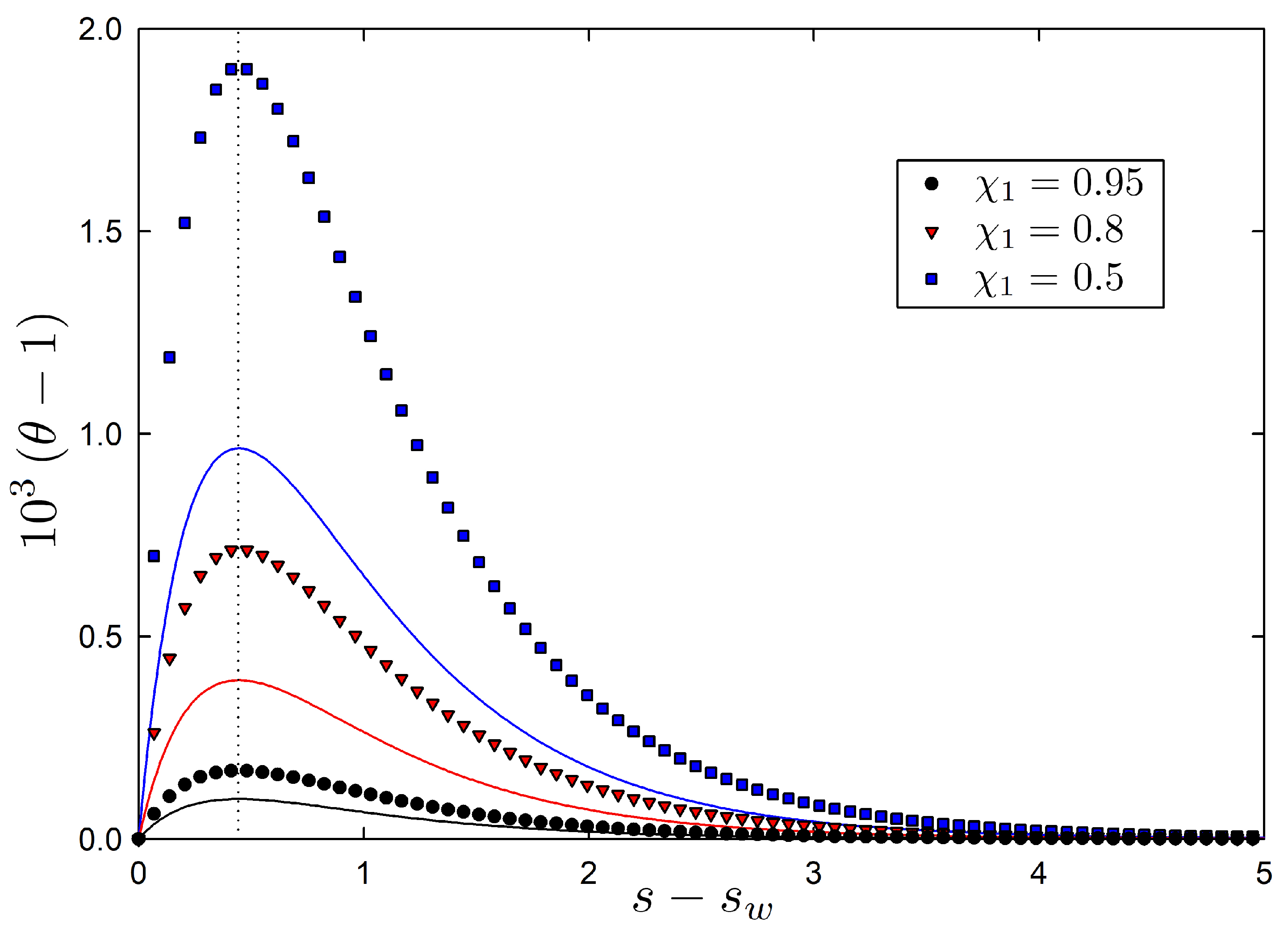
3.3. Kovacs Hump in Linear Response

Now, we look into the Kovacs hump in the linear response approximation. Following the discussion leading to Equation (20), first we have to calculate the relaxation function ϕ T for the granular temperature. The system is at the steady state corresponding to a driving ξ 0 for t < 0 ; at t = 0 , the driving is instantaneously changed to ξ , and only the linear terms in Δ ξ = ξ ξ 0 are retained. We choose the normalization of ϕ T ( s ) in such a way that ϕ T ( 0 ) = 1 , that is:
ϕ T ( s ) lim Δ T ( 0 ) 0 Δ T ( s ) Δ T ( 0 ) = lim Δ θ ( 0 ) 0 Δ θ ( s ) Δ θ ( 0 ) .
Since T s changes with ξ , but a 2 does not, we have to solve Equation (44) for Δ a 2 ( 0 ) = 0 and arbitrary (small enough) Δ θ ( 0 ) . The solution is:
ϕ T ( s ) = c + e λ + s + c e λ s ,
c + = M 11 λ λ + λ , c = λ + M 11 λ + λ ,
where M i j is the ( i , j ) element of the matrix M and λ ± its eigenvalues,
λ ± = T r M ± ( T r M ) 2 4 det M 2 = T r M ± ( M 11 M 22 ) 2 + 4 M 12 M 21 2 .
Both eigenvalues λ ± are negative, since T r M < 0 and det M > 0 for all β > 0 . Therefore, | λ + | < | λ | , and it is λ + that dominates the relaxation of the granular temperature for long times. Moreover, c ± > 0 , and thus, the linear relaxation function ϕ T ( s ) is always positive and decays monotonically to zero.
Next, we consider a Kovacs-like experiment: the system was at the NESS corresponding to a driving ξ 0 , with granular temperature T s , 0 for t < 0 ; the driving is suddenly changed to ξ 1 at t = 0 so that the system starts to relax towards a new steady temperature T s , 1 for 0 t t w , and this relaxation is interrupted at t = t w , because the driving is again suddenly changed to the value ξ such that the stationary granular temperature T s equals its instantaneous value at t w . The time evolution of the granular temperature for t t w is given by the particularization of Equations (20) and (21) to our situation, that is,
K T ( s ) = ξ 0 ξ 1 ξ 0 ξ ϕ T ( s ) ξ ξ 1 ξ 0 ξ ϕ T ( s s w ) , ξ ξ 1 ξ 0 ξ 1 = ϕ T ( s w ) ,
where we have made use of the normalization ϕ T ( 0 ) = 1 . In the linear response approximation, the jumps in the driving values can be substituted by the corresponding jumps in the stationary values of the granular temperature.
The structure of the linear relaxation function ϕ T ( s ) , as a linear combination of decreasing exponentials exp ( λ ± t ) , λ ± < 0 , with positive weights c ± , assures that the Kovacs behavior is normal: (i) K T ( s ) is always positive and bounded from above by ϕ T ( s ) and (ii) there is only one maximum at a certain time s k > s w [6]. The anomalous behavior found in the uniformly heated hard-sphere granular for large enough inelasticity is thus not present here. This is consistent with the quasi-elastic limit we have introduced to simplify the collision operator.

3.4. Nonlinear Kovacs Hump

Here, we consider the Kovacs hump for arbitrary large driving jumps. In our model, we can make use of the smallness of a 2 , which is assumed in the first Sonine approximation, in order to introduce a perturbative expansion of Equations (42) in powers of a 2 s . The procedure is completely analogous to that performed in [12,13] for a dilute gas of inelastic hard spheres, and thus, we omit the details here.
We start by writing a 2 = a 2 s A 2 , with A 2 of the order of unity, and:
θ ( s ) = θ 0 ( s ) + a 2 s θ 1 ( s ) + , A 2 ( s ) = A 20 ( s ) + a 2 s A 21 ( s ) + .
These expansions are inserted into Equations (42), which have to be solved with initial conditions θ ( s w ) = 1 , A 2 ( s w ) = A 2 ini . To the lowest order, θ 0 ( s ) = 1 , whereas A 20 ( s ) decays exponentially to one,
A 20 ( s ) 1 A 2 ini 1 e κ 2 s s w .
In order to describe the Kovacs hump, we compute θ 1 ( s ) that verifies the differential equation:
d θ 1 d s = 1 + β 2 θ 1 + β ( 2 + β ) 16 A 20 1 ,
which can be immediately integrated to give:
θ ( s ) 1 a 2 ini a 2 s β ( 2 + β ) 8 ( 2 + β 2 κ 2 ) e κ 2 s s w e 1 + β 2 s s w , s s w ,
The structure of this result is completely analogous to those in [12,13], and thus, the conclusions can also be drawn in a similar way. In particular, we want to highlight that (i) the factor that controls the size of the hump is proportional to a 2 ini a 2 s and (ii) the shape of the hump is codified in the factor between brackets that only depends on β . Note that ( a 2 ini a 2 s ) > 0 for the cooling protocols ( ξ 1 < ξ < ξ 0 ) considered here, and thus, no anomalous Kovacs hump is expected in the nonlinear regime either.

4. Numerical Results

Here, we compare the theoretical approach above to numerical results of our model. Specifically, we focus on the case β = 1 that gives a collision rate similar to that of hard-spheres. All simulations have been carried out with a restitution coefficient α = 0 . 999 , which corresponds to the quasi-elastic limit in which our simplified kinetic description holds. Furthermore, we set ω = 1 without loss of generality.

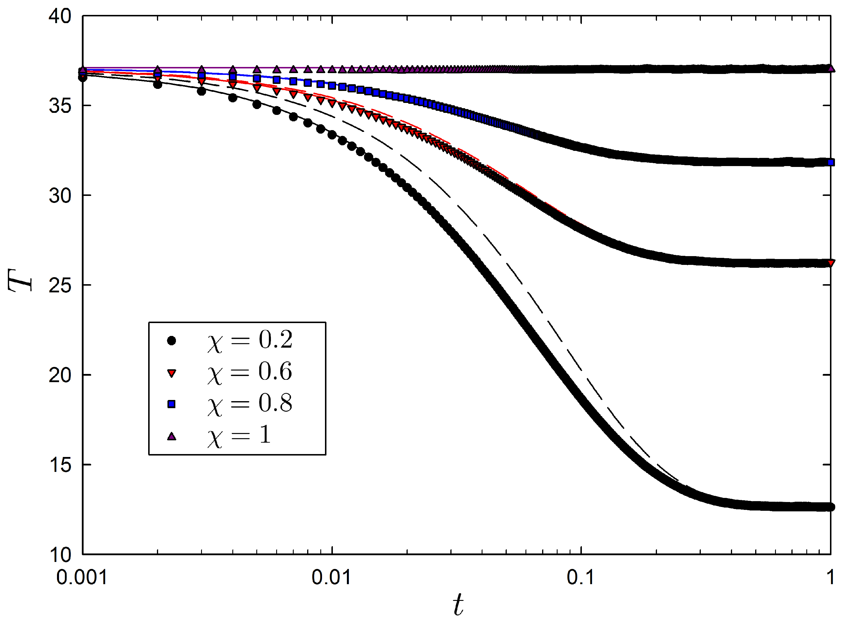
4.1. Validation of the Evolution Equations and Linear Relaxation
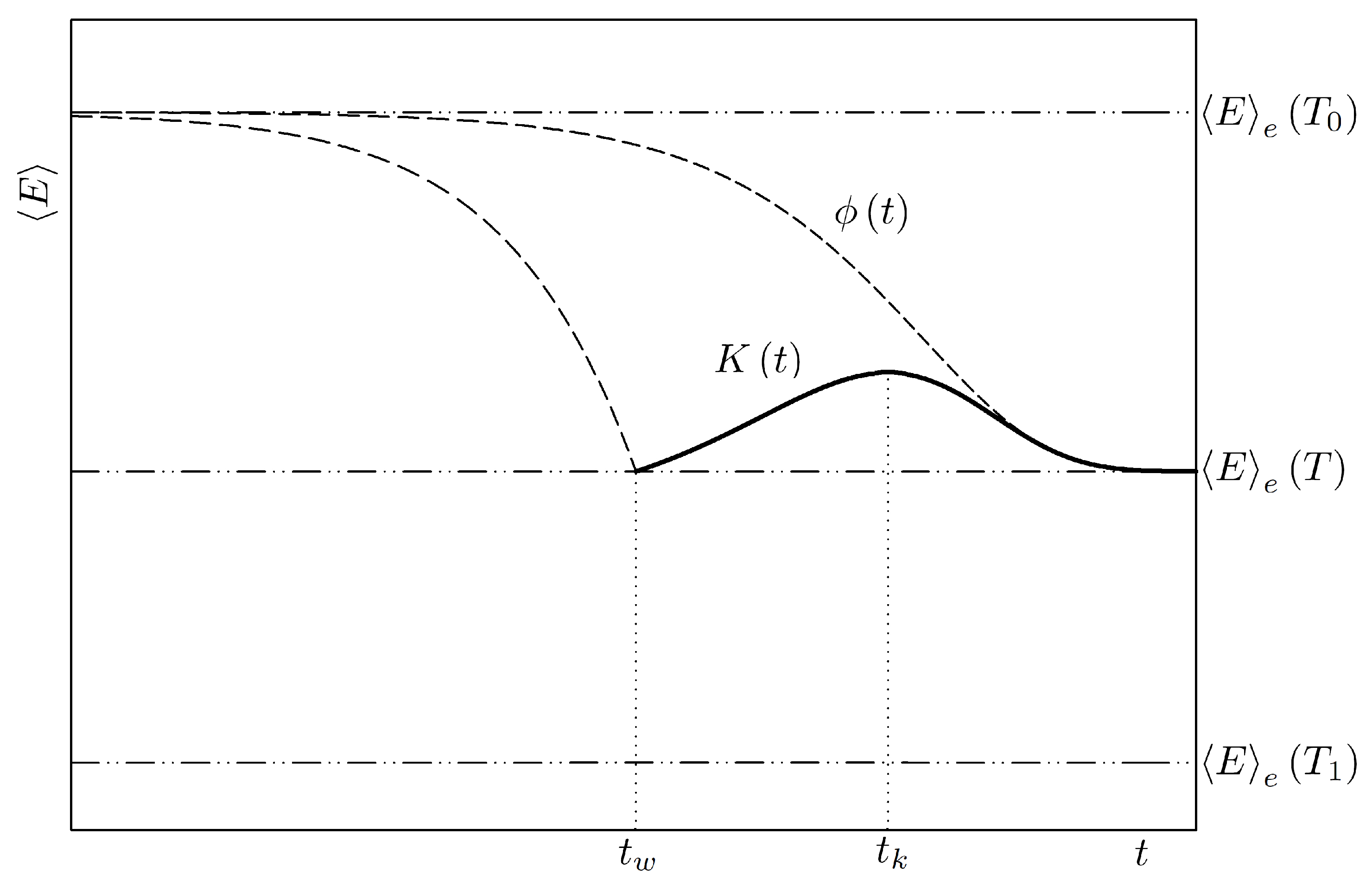
First of all, we check the validity of the first Sonine approximation, as given by Equations (38), to describe the time evolution of our system. In order to do so, we compare several relaxation curves between the NESS corresponding to two different noise strengths. In particular, we always depart from the stationary state corresponding to χ 0 = 1 and afterwards let the system evolve with χ = { 0.2 , 0.6 , 0.8 , 1 } for t > 0 . In Figure 2, we compare the Monte Carlo simulation (see Appendix A for details) of the system with the numerical solution of the evolution equations in the first Sonine approximation (38). In addition, we also have plotted the analytical solution of the linear response system, Equation (44). The agreement is complete between simulation and theory, and it can be observed how the linear response result becomes more accurate as the temperature jump decreases.
In order not to clutter the plot in Figure 2, we have not shown the results for the nonlinear first Sonine approximation, Equation (37). The relative error between their numerical solution and that of the standard first Sonine approximation (38) is at most of order 0.1 % , for all the cases we have considered. Henceforth, we always use the latter, which is the usual approach in kinetic theory.

4.2. Kovacs Hump

Since the numerical integration of the first Sonine approximation perfectly agrees with Monte Carlo simulations, we compare the analytical results for the Kovacs hump with the former. Specifically, we work in reduced variables, and therefore, we integrate numerically Equations (42).

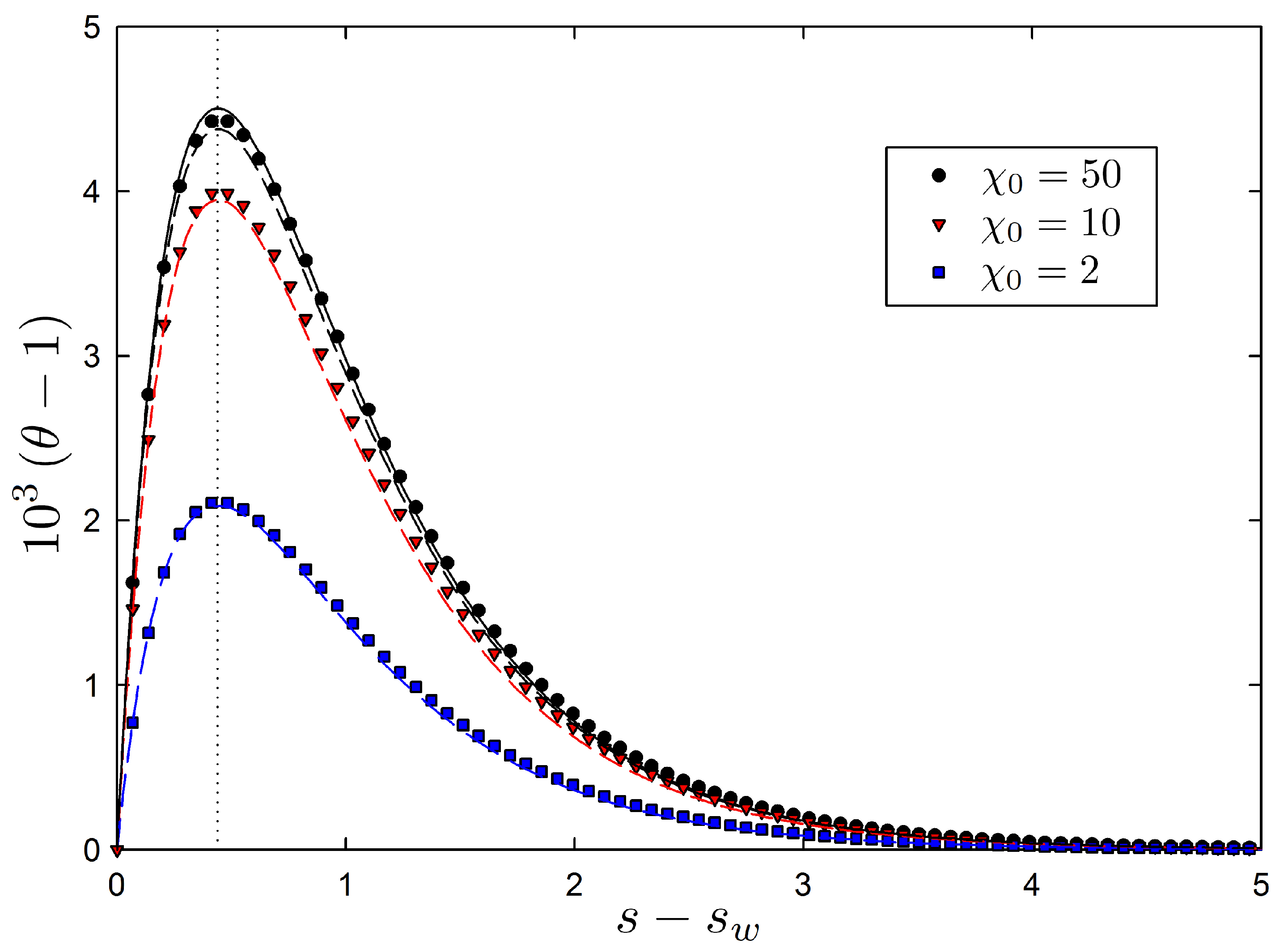
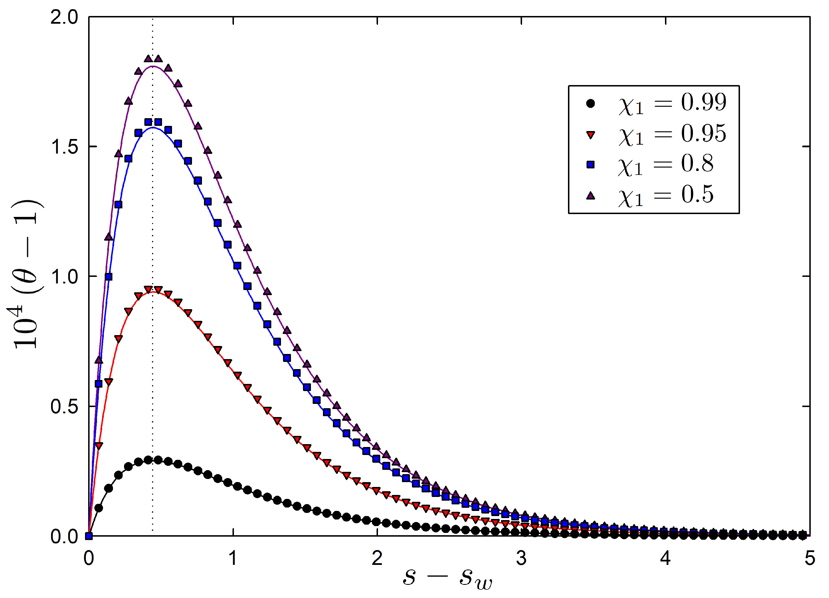
4.2.1. Linear Response

It is convenient to rewrite the expression for the Kovacs hump in an alternative form to compare our theory to numerical results. We take advantage of the simple structure of the relaxation function in the first Sonine approximation, which is the sum of two exponentials, to introduce the factorization [6]:
K T ( s ) = K 0 ( s w ) K 1 ( s s w ) ,
where:
K 0 ( s w ) = c + c e λ + s w e λ s w 1 ϕ T ( s w ) , K 1 ( s s w ) = e λ + ( s s w ) e λ ( s s w ) .
Firstly, this factorization property shows that the position s k of the maximum relative to the waiting time s w , that is, s k s w , is controlled by the function K 1 . Thus, s k s w does not depend on the waiting time, but only on the two eigenvalues λ ± . Namely,
s k s w = 1 λ + λ ln λ λ + β = 1 0.442 .
Secondly, the height of the maximum K max does depend on the waiting time s w due to the factor K 0 ( s w ) . Specifically, it can be shown that K max is a monotonically decreasing function of the waiting time s w that vanishes in the limit as s w .
In order to check the above results, we have fixed the initial and final drivings in the Kovacs protocol χ 0 and χ and changed the intermediate driving value χ 1 . We do so to simplify the comparison, because the time scale s involves the steady value of the temperature; see Equation (41). Note that the smaller χ 1 is, the shorter the waiting time becomes. Therefore, one expects to get a Kovacs hump whose maximum remains at s s w 0.44 , but raises as χ 1 decreases. This is shown in Figure 3, where the numerical solution of the first Sonine approximation equations (42) and the analytical result (53) are compared. Their agreement is almost perfect for the two lowest curves, corresponding to χ 1 = 0.99 and χ 1 = 0.95 , as expected, but is still remarkably good for the two topmost ones, corresponding to the not-so-small jumps for χ 1 = 0.8 and χ 1 = 0.5 .

4.2.2. Nonlinear Regime

Furthermore, we explore the Kovacs effect out of the linear regime. Figure 4 is similar to Figure 3, but for larger temperature (or driving) jumps. We have also fixed the initial and final values of the driving, χ 0 = 10 and χ = 1 . The intermediate values of the driving are the same as in the linear case except for the largest one, χ 1 = 0.99 , which we have omitted for the sake of clarity (its hump is too small in the scale of the figure). Now, the linear response theory results just provide the qualitative behavior of the hump, correctly predicting the position of the maximum, but not its height. On the one hand, and consistent with the numerical results in an active matter model [15], the Kovacs hump out of the linear response regime is larger than the prediction of linear response theory. On the other hand, the position of the maximum remains basically unchanged, and its height still increases as χ 1 decreases.
We also compare our analytical expansion in a 2 s with the numerical solutions of Equations (42) for large jumps. Specifically, in order to make things as simple as possible, we choose χ 1 = 0 . If the waiting time is long enough, the system reaches the homogeneous cooling state and a 2 ( s w ) = a 2 HCS , which is then the initial condition for the final stage of the Kovacs protocol. Moreover, we can compute the location of the maximum of the hump from Equation (52), obtaining:
s k s w = 2 κ 2 2 β ln 2 κ 2 2 + β β = 1 0.437 .
This result is numerically indistinguishable from that of linear response, as given by Equation (54), since the relative error is around 1 % .
In Figure 5, we put forward a comparison between the Kovacs hump obtained from the numerical solution of the first Sonine approximation equations and our theoretical expression for the nonlinear regime, Equation (52). Fixing ξ 1 = 0 and ξ = 1 , as ξ 0 increases (as the waiting time is increased), the hump approaches Equation (52) with a 2 ini = a 2 HCS . Moreover, our theory perfectly reproduces all the numerical curves when we substitute the actual values of a 2 ini into Equation (52).

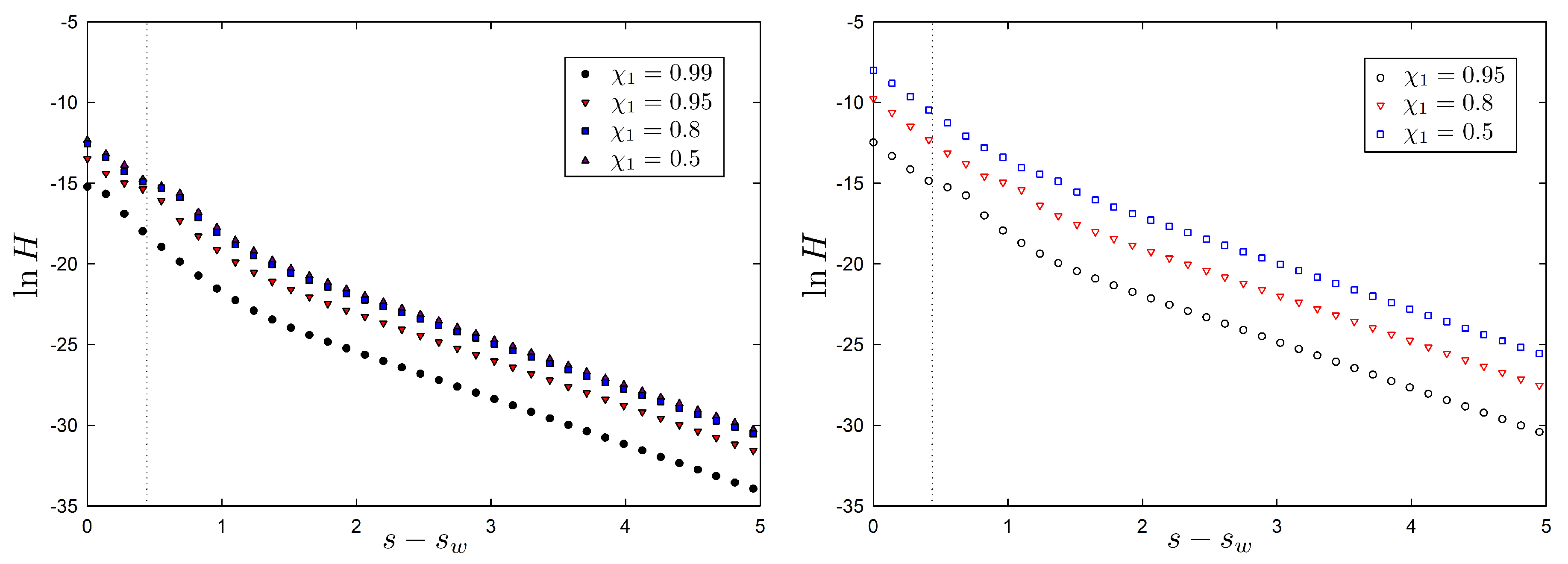
4.3. Monotonicity of an H-Functional

The non-monotonicity in the relaxation of the granular temperature that is brought about by the Kovacs protocol is not automatically transferred to other relevant physical magnitudes. Specifically, here, we deal with the H-functional:
H ( t ) = + d v f ( v , t ) log f ( v , t ) f s ( v ) ,
There is strong numerical evidence about H ( t ) being a Lyapunov functional for granular fluids, thus allowing it to be considered as an out-of-equilibrium entropy relative to that of the NESS, in this context [19,20]. Moreover, it has been analytically proven that H ( t ) is a Lyapunov functional in our system for the Maxwell collision rule β = 0 [21].
We have computed H ( t ) numerically from Equation (56) within the first Sonine approximation (that is, we have substituted both f ( v , t ) and f s ( v ) by their expressions in the first Sonine approximation and calculated the integral numerically) for the Kovacs protocols considered in Figure 3 and Figure 4. Once more, we have taken β = 1 , for which the analytical proof in [21] does not hold. The results are shown in Figure 6 and make it clear that H ( t ) still monotonically decreases for the Kovacs-like protocols, in both the linear (left panel) and nonlinear (right panel) regimes. At the time of the maximum in the hump, s s w 0.44 , no special signature is observed in the entropy.

5. Discussion

One of the main results in our paper is the extension of the linear response expression for the Kovacs hump in thermal systems, as given by Equations (1) and (2), to the realm of athermal systems, Equations (20) and (21). This extension is (i) not trivial, since athermal systems tend in the long time limit to an NESS, not to an equilibrium state, and (ii) very general, since it can be done starting from the evolution equations at either the mesoscopic or the macroscopic level of description. Therefore, it means that a Kovacs-like effect is to be expected for a very wide class of physical properties Y in a very wide class of systems, basically as long as the relaxation function ϕ Y ( t ) to the NESS is monotonic.
This theoretical result has been checked in a class of systems that mimic the dynamics of the shear component of the velocity of a granular fluid. In the linear response regime, we have found a good agreement between the theoretical prediction and the numerical results. Furthermore, we have investigated how the linear response result extends to the nonlinear regime. In this region, the linear response theory results remain useful at a qualitative level, but the actual values for the hump lie well above the linear prediction. Interestingly, this kind of giant Kovacs hump has been recently reported in active systems [15]. In addition, the nonlinear Kovacs hump can be theoretically explained by an expansion in the excess kurtosis.
Our work also opens new interesting perspectives for future research. Remarkably, the Kovacs-like memory effects analyzed here involve only jump protocols for the control parameter, which is time-independent both in the waiting time window 0 < t < t w (value ξ 1 ) and in the return to stationarity region t > t w (value ξ ). Very recently, the response of the system to continuous perturbations [31,32] has been studied, which raises the interesting question of building up a theory, similar to ours, in which the control is continuously varied up to t w in a first stage and then abruptly changed to the value that corresponds to the stationary value of the relaxing physical observable. To the best of our knowledge, a thorough study of this kind of response is lacking. Moreover, the analysis of the nonlinear response in light of generalized fluctuation-dissipation relations [33] is worthy of consideration.
On another note, our analysis of the Kovacs effect in the model, being restricted to the quasi-elastic limit, has not found the anomalous behavior shown by a gas of inelastic hard spheres for large enough inelasticity in the nonlinear regime [12,13]. The possibility of such a behavior in linear response, either in the model or in the granular gas, deserves further investigation. In addition, our work clearly shows the compatibility of the non-monotonic decay of the granular temperature (or the corresponding relevant physical variable) and the monotonic decay of the nonequilibrium entropy or H-functional [19,20,21,34]. In this respect, to elucidate if the hump leaves some signature in the decay of the nonequilibrium entropy is compelling.

Acknowledgments

We acknowledge the support of the Spanish Ministerio de Economía y Competitividad through Grant FIS2014-53808-P. Carlos A. Plata also acknowledges the support from the FPUFellowship Programme of the Spanish Ministerio de Educación, Cultura y Deporte through Grant FPU14/00241.

Author Contributions

All authors contributed equally to this work. All authors have read and approved the final manuscript.

Conflicts of Interest

The authors declare no conflict of interest. The founding sponsors had no role in the design of the study; in the collection, analyses or interpretation of data; in the writing of the manuscript; nor in the decision to publish the results.

Appendix A. Simulation Algorithm

We have made use of a residence time algorithm that gives the numerical integration of a master equation in the limit of infinite trajectories [35,36]. The basic numerical recipe is as follows:
  • At time τ , a random “free time” τ f > 0 is extracted with an exponential probability density Ω ( v ) exp [ Ω ( v ) τ f ] , where Ω ( v ) = l ω | v l v l + 1 | β depends on the state of the system v ;
  • Time is advanced by such a free time τ τ + τ f ;
  • A pair ( l , l + 1 ) is chosen to collide with probability ω | v l v l + 1 | β / Ω ( v ) ;
  • All particles are heated by the stochastic thermostat, by adding independent Gaussian random numbers of zero mean and variance χ τ f to their velocities;
  • In order to conserve momentum, the mean value of the random numbers generated in the previous step is subtracted from the velocities of all particles;
  • The process is repeated from Step 1.

References

  1. Kovacs, A.J.; Aklonis, J.J.; Hutchinson, J.M.; Ramos, A.R. Isobaric volume and enthalpy recovery of glasses. II. A transparent multiparameter theory. J. Polym. Sci. 1979, 17, 1097–1162. [Google Scholar] [CrossRef]
  2. Bertin, E.M.; Bouchaud, J.P.; Drouffe, J.M.; Godreche, C. The Kovacs effect in model glasses. J. Phys. A 2003, 36, 10701. [Google Scholar] [CrossRef]
  3. Buhot, A. Kovacs effect and fluctuation–dissipation relations in 1D kinetically constrained models. J. Phys. A 2003, 36, 12367. [Google Scholar] [CrossRef]
  4. Mossa, S.; Sciortino, F. Crossover (or Kovacs) effect in an aging molecular liquid. Phys. Rev. Lett. 2004, 92, 045504. [Google Scholar] [CrossRef] [PubMed]
  5. Aquino, G.; Leuzzi, L.; Nieuwenhuizen, T.M. Kovacs effect in a model for a fragile glass. Phys. Rev. B 2006, 73, 094205. [Google Scholar] [CrossRef]
  6. Prados, A.; Brey, J.J. The Kovacs effect: A master equation analysis. J. Stat. Mech. 2010, 2010, 368–369. [Google Scholar] [CrossRef]
  7. Diezemann, G.; Heuer, A. Memory effects in the relaxation of the Gaussian trap model. Phys. Rev. E 2011, 83, 031505. [Google Scholar] [CrossRef] [PubMed]
  8. Ruiz-García, M.; Prados, A. Kovacs effect in the one-dimensional Ising model: A linear response analysis. Phys. Rev. E 2014, 89, 012140. [Google Scholar] [CrossRef] [PubMed]
  9. Van Kampen, N.G. Stochastic Processes in Physics and Chemistry; North-Holland: Amsterdam, The Netherlands, 1992. [Google Scholar]
  10. Pöschel, T.; Luding, S. Granular Gases Vol. 564 of Lecture Notes in Physics; Springer: Berlin/Heidelberg, Germany, 2001. [Google Scholar]
  11. Van Noije, T.P.C.; Ernst, M.H. Velocity distributions in homogeneous granular fluids: The free and the heated case. Granul. Matter 1998, 1, 57–64. [Google Scholar] [CrossRef]
  12. Prados, A.; Trizac, E. Kovacs-Like Memory Effect in Driven Granular Gases. Phys. Rev. Lett. 2014, 112, 198001. [Google Scholar] [CrossRef] [PubMed]
  13. Trizac, E.; Prados, A. Memory effect in uniformly heated granular gases. Phys. Rev. E 2014, 90, 012204. [Google Scholar] [CrossRef] [PubMed]
  14. Lahini, Y.; Gottesman, O.; Amir, A.; Rubinstein, S.M. Nonmonotonic Aging and Memory Retention in Disordered Mechanical Systems. Phys. Rev. Lett. 2017, 118, 085501. [Google Scholar] [CrossRef] [PubMed]
  15. Kürsten, R.; Sushkov, V.; Ihle, T. Giant Kovacs-Like Memory Effect for Active Particles. Phys. Rev. Lett. 2017, in press. [Google Scholar]
  16. Lasanta, A.; Manacorda, A.; Prados, A.; Puglisi, A. Fluctuating hydrodynamics and mesoscopic effects of spatial correlations in dissipative systems with conserved momentum. New J. Phys. 2015, 17, 083039. [Google Scholar] [CrossRef]
  17. Manacorda, A.; Plata, C.A.; Lasanta, A.; Puglisi, A.; Prados, A. Lattice Models for Granular-Like Velocity Fields: Hydrodynamic Description. J. Stat. Phys. 2016, 164, 810–841. [Google Scholar] [CrossRef]
  18. Plata, C.A.; Manacorda, A.; Lasanta, A.; Puglisi, A.; Prados, A. Lattice models for granular-like velocity fields: Finite-size effects. J. Stat. Mech. 2016, 2016, 093203. [Google Scholar] [CrossRef]
  19. Marconi, U.M.B.; Puglisi, A.; Vulpiani, A. About an H-theorem for systems with non-conservative interactions. J. Stat. Mech. 2013, 2013, 114–124. [Google Scholar] [CrossRef]
  20. García de Soria, M.I.; Maynar, P.; Mischler, S.; Mouhot, C.; Rey, T.; Trizac, E. Towards an H-theorem for granular gases. J. Stat. Mech. 2015, 2014, P11009. [Google Scholar] [CrossRef]
  21. Plata, C.A.; Prados, A. Global stability and H-theorem in lattice models with nonconservative interactions. Phys. Rev. E 2017, 95, 052121. [Google Scholar] [CrossRef] [PubMed]
  22. Brey, J.J.; Prados, A. Stretched exponential decay at intermediate times in the one-dimentional Ising model at low temperatures. Physica A 1993, 197, 569–582. [Google Scholar] [CrossRef]
  23. Prasad, V.V.; Sabhapandit, S.; Dhar, A.; Narayan, O. Driven inelastic Maxwell gas in one dimension. Phys. Rev. E 2017, 95, 022115. [Google Scholar] [CrossRef] [PubMed]
  24. Ben-Naim, E.; Krapivsky, P.L. The inelastic Maxwell model. In Granular Gas Dynamics; Pöschel, T., Brilliantov, N., Eds.; Lecture Notes in Physics; Springer: Berlin/Heidelberg, Germany, 2003; Volume 624, pp. 65–94. [Google Scholar]
  25. Ernst, M.H.; Trizac, E.; Barrat, A. The rich behavior of the Boltzmann equation for dissipative gases. EPL 2006, 76, 56–62. [Google Scholar] [CrossRef]
  26. Montanero, J.M.; Santos, A. Computer simulation of uniformly heated granular fluids. Granul. Matter 2000, 2, 53–64. [Google Scholar] [CrossRef]
  27. Maynar, P.; García de Soria, M.I.; Trizac, E. Fluctuating hydrodynamics for driven granular gases. Eur. Phys. J. Spec. Top. 2009, 179, 123–139. [Google Scholar] [CrossRef]
  28. Prasad, V.V.; Sabhapandit, S.; Dhar, A. High-energy tail of the velocity distribution of driven inelastic Maxwell gases. EPL 2013, 104, 54003. [Google Scholar] [CrossRef]
  29. Plata, C.A.; Prados, A. Kinetic description of a class of systems with non-conservative interactions. 2018; unpublished. [Google Scholar]
  30. Abramowitz, M.; Stegun, I.A. Handbook of Mathematical Functions; Dover: New York, NY, USA, 1972. [Google Scholar]
  31. Falasco, G.; Baiesi, M. Temperature response in nonequilibrium stochastic systems. EPL 2016, 113, 20005. [Google Scholar] [CrossRef]
  32. Falasco, G.; Baiesi, M. Nonequilibrium temperature response for stochastic overdamped systems. New J. Phys. 2016, 18, 043039. [Google Scholar] [CrossRef]
  33. Lippiello, E.; Corberi, F.; Sarracino, A.; Zannetti, M. Nonlinear response and fluctuation-dissipation relations. Phys. Rev. E 2008, 78, 041120. [Google Scholar]
  34. Brey, J.J.; Prados, A. Normal solutions for master equations with time-dependent transition rates: Application to heating processes. Phys. Rev. E 1993, 47, 1541. [Google Scholar] [CrossRef]
  35. Bortz, A.B.; Kalos, M.H.; Lebowitz, J.L. A new algorithm for Monte Carlo simulation of Ising spin systems. J. Comput. Phys. 1975, 17, 10–18. [Google Scholar] [CrossRef]
  36. Prados, A.; Brey, J.J.; Sánchez-Rey, B. A dynamical Monte Carlo algorithm for master equations with time-dependent transition rates. J. Stat. Phys. 1997, 89, 709–734. [Google Scholar] [CrossRef]
Figure 1. Scheme of the Kovacs experiment described in the text. The dashed curve on the right, labeled by ϕ ( t ) , represents the direct relaxation from T 0 to T. The dashed curve on the left stands for the part of the relaxation from T 0 to T 1 that is interrupted at t = t w by the second temperature jump, changing abruptly the temperature from T 1 to T. After this second jump, the system follows the non-monotonic response K ( t ) (solid line), which reaches a maximum at t = t k and, afterwards, approaches ϕ ( t ) for very long times.
Entropy 19 00539 g001
Figure 2. (Color online) Direct relaxation of the granular temperature T for different final noise amplitudes. All curves start from the stationary state corresponding to χ 0 = 1 . We compare Monte Carlo simulation results for a system of N = 100 sites (symbols) with the numerical solution of the first Sonine approximation, Equation (38) (solid lines), and the analytic solution of the linear response system, Equation (44) (dashed lines).
Entropy 19 00539 g002
Figure 3. (Color online) Kovacs hump in linear response. We have fixed the initial and final drivings, χ 0 = 1.05 and χ = 1 , and considered four values for the intermediate driving χ 1 = { 0.5 , 0.8 , 0.95 , 0.99 } . The linear response theory result (53) (solid line) perfectly agrees with the numerical solution of the first Sonine approximation (symbols), Equation (42). Furthermore, the theoretical prediction for the maximum (54), which again agrees with the numerical results, is plotted (dotted line).
Entropy 19 00539 g003
Figure 4. (Color online) Kovacs hump out of the linear regime. The initial driving is much higher than that in Figure 3, χ 0 = 10 , whereas the final and intermediate values of the driving are again χ = 1 and χ 1 = { 0.5 , 0.8 , 0.95 } . The linear response theoretical expression (48) (solid line) remains quite below the numerical solutions of the first Sonine approximation (42) (symbols). The theoretical expression for the maximum in linear response (54) (dotted line) still gives a good description thereof; see also Figure 5.
Entropy 19 00539 g004
Figure 5. (Color online) Kovacs hump in the nonlinear regime and prediction of the perturbative expansion in a 2 s . We have considered the following values of the drivings: χ 0 = { 2 , 10 , 50 } , χ 1 = 0 and χ = 1 . Symbols stand for the numerical solutions of the first Sonine approximation (42), whereas lines correspond to the theoretical expression (52). For the solid line, a 2 ini = a 2 HCS , while for the dashed lines, we have used the value of a 2 ini in the numerical solution. A perfect agreement is observed. Finally, we have plotted the theoretical expression for the maximum position in nonlinear response (dotted line), Equation (55), which also shows an excellent agreement with numerics.
Entropy 19 00539 g005
Figure 6. (Color online) Time evolution of the H-functional. The relaxation of H is shown to be monotonic even for Kovacs-like experiments. The left and right panels correspond to the protocols in Figure 3 (filled symbols) and Figure 4 (open symbols), that is to the linear and nonlinear regimes. The vertical dotted line marks the theoretical position of the maximum in the corresponding regime.
Entropy 19 00539 g006

