1. Introduction
Often, one needs in studies in nonlinear dynamics and statistical physics to investigate the dynamical properties of a many-body interacting Hamiltonian system evolving under the condition of a constant temperature. For example, one might be interested in studying the dynamical properties of the system in canonical equilibrium at a certain temperature
T, with the temperature being proportional to the average kinetic energy of the system by virtue of the Theorem of Equipartition (In this work, we measure temperatures in units of the Boltzmann constant). To this end, one may devise a dynamics having a temperature
as a dynamical parameter that is designed to relax an initial configuration of the system to canonical equilibrium at temperature
, and then make the choice
. A common practice is to employ a Langevin dynamics, i.e., a
noisy, dissipative dynamics that mimics the interaction of the system with an external heat bath at temperature
in terms of a deterministic frictional force and an uncorrelated, Gaussian-distributed random force added to the equation of motion [
1]. In this approach, one then tunes suitably the strength of the random force such that the Langevin dynamics relaxes at long times to canonical equilibrium at temperature
. The presence of dissipation renders the dynamics to be
irreversible in time. A complementary approach to such a noisy, dissipative dynamics was pioneered by Nosé and Hoover, in which the dynamics is fully
deterministic and
time-reversible, while achieving the same objective of relaxing the system to canonical equilibrium at the desired temperature
[
2,
3]; for a review, see [
4,
5]. The time evolution under the condition of relaxation at long times to canonical equilibrium at a given temperature is said to represent isokinetic ensemble dynamics when taking place according to the Nosé–Hoover equation of motion and to represent Langevin/canonical ensemble dynamics when taking place following the Langevin equation of motion.
To illustrate in detail the distinguishing feature of the Nosé–Hoover vis-à-vis Langevin dynamics, consider an interacting
N-particle system characterized by the set
of canonical coordinates and conjugated momenta. The particles, which we take for simplicity to have the same mass
m, interact with one another via the two-body interaction potential
. In the following, we consider
’s and
’s to be one-dimensional variables for reasons of simplicity. Our analysis, however, extends straightforwardly to higher dimensions. The Hamiltonian of the system is given by
where the first term on the right-hand side stands for the kinetic energy of the system.
In the approach due to Langevin, the dynamical equations of the system are given by
where
t denotes time,
is the dissipation constant, while
is a Gaussian, white noise satisfying
Here, the overbars denote averaging over noise realizations, while
characterizes the strength of the noise. The dynamics (
2) are evidently not time-reversal invariant. Choosing
ensures that the dynamics (
2) relaxes at long times to the canonical distribution at
given by [
1]
in which the kinetic energy density of the system fluctuates around the average value
.
In the approach due to Nosé and Hoover, a degree of freedom
s augmenting the set
is introduced, which is taken to characterize an external heat reservoir that interacts with the system through the momenta
’s. The Hamiltonian of the combined system is given by
where
Q is the mass and
is the conjugated momentum of the additional degree of freedom. The dynamics of the system is given by the following Hamilton equations of motion:
It may be easily checked that unlike dynamics (
2), dynamics (
6) is invariant under time reversal. In terms of new variables
and rescaled time
one obtains from the Hamilton Equations (
6) the following dynamics:
where
is the kinetic energy, while we have defined
From Equations (
9)–(
12), we observe that a complete description of the time evolution of the system is given in terms of Equations (
9), (
10), and (
12), without any reference to Equation (
11) for
s, so that, as far as the description of the system is concerned, the variable
s is an irrelevant one that may be ignored. We note in passing that a different, but closely related, Hamiltonian giving directly the Nosé-Hoover equations of motion but without any time scaling, as in Equation (
8), is discussed in [
6]. We will from now on drop the tilde over time in order not to overload the notation. Let us note that, in terms of the variables
’s, the Hamiltonian (
5) takes the form
From Equation (
12), we find that, in the stationary state
), the kinetic energy of the system equals
(the extra factor of unity takes care of the presence of the additional degree of freedom
s). For large
, we then have the desired result: an ensemble of initial conditions under the evolution given by Equations (
9), (
10), and (
12) evolves at long times to a stationary state in which the average kinetic energy density has the value
. The quantity
in Equation (
12) denotes a relaxation timescale over which the kinetic energy relaxes to its target value. Beyond the average kinetic energy, it has been demonstrated by invoking the phase space continuity equation that the distribution
is a stationary state of the Nosé–Hoover dynamics [
3]. It then follows that the corresponding stationary distribution for the system variables
is the canonical equilibrium distribution:
normalized as
. Thus, the dynamics (
9)–(
12) that includes the additional dynamical variable
s nevertheless preseves the canonical equilibrium distribution of the system. A general formalism for constructing modified Hamiltonian dynamical systems that preserve a canonical equilibrium distribution on adding a time evolution equation for a single additional thermostat variable is discussed in [
7].
Equation (
16) implies that the single-particle momentum distribution
, defined such that
gives the probability that a randomly chosen particle has its momentum between
p and
, is a Gaussian distribution with mean zero and width equal to
:
Consequently, the moments
, with
, satisfy
.
In the above backdrop, the principal objective of this work is to answer the question: what is the effect of inter-particle interactions on the relaxation properties of the Nosé–Hoover dynamics? More specifically, considering a system embedded in a d-dimensional space, we ask: do systems with long-range interactions, in which the inter-particle interaction decays slower than , behave in a similar way to short-range systems that have the inter-particle interaction decaying faster than ? How does the timescale over which the phase space distribution relaxes to its canonical equilibrium form behave in the two cases, and, in particular, is there a system-size dependence in the timescale for long-range systems with respect to short-range ones? Studying these issues is particularly relevant and timely in the wake of recent surge in interest across physics in long-range interacting (LRI) systems.
LRI systems may display a notably distinct thermodynamic behavior with respect to short-range ones [
8,
9,
10,
11,
12]. These systems are characterized by a two-body interaction potential
that decays asymptotically with inter-particle separation
r as
, with
in
d spatial dimensions. The limit
corresponds to the case of mean–field interaction. Examples of LRI systems are self-gravitating systems, plasmas, fluid dynamical systems, and some spin systems. One of the striking dynamical features resulting from long-range interactions is the occurrence of non-equilibrium quasi-stationary states (QSSs) during relaxation of LRI systems towards equilibrium. These states have lifetimes that diverge with the number of particles constituting the system, so that, in the thermodynamic limit, the system remains trapped in QSSs and does not attain equilibrium. Only for a finite number of particles do the QSSs eventually evolve towards equilibrium. Even in equilibrium, LRI systems may exhibit features such as ensemble inequivalence and a negative heat capacity in the microcanonical ensemble that are unusual for short-range systems.
In this work, we address our aforementioned queries within the ambit of a model system comprising classical
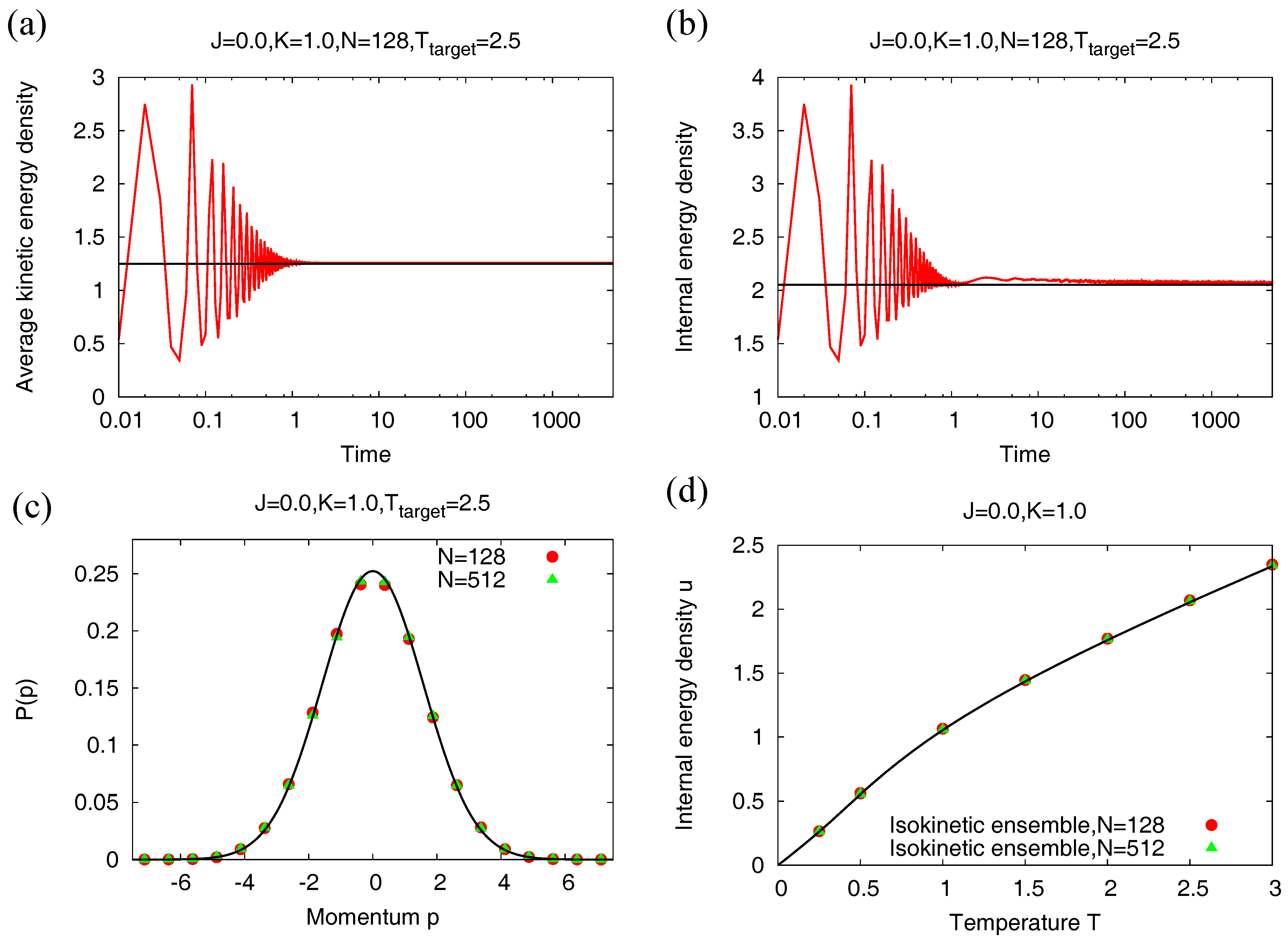
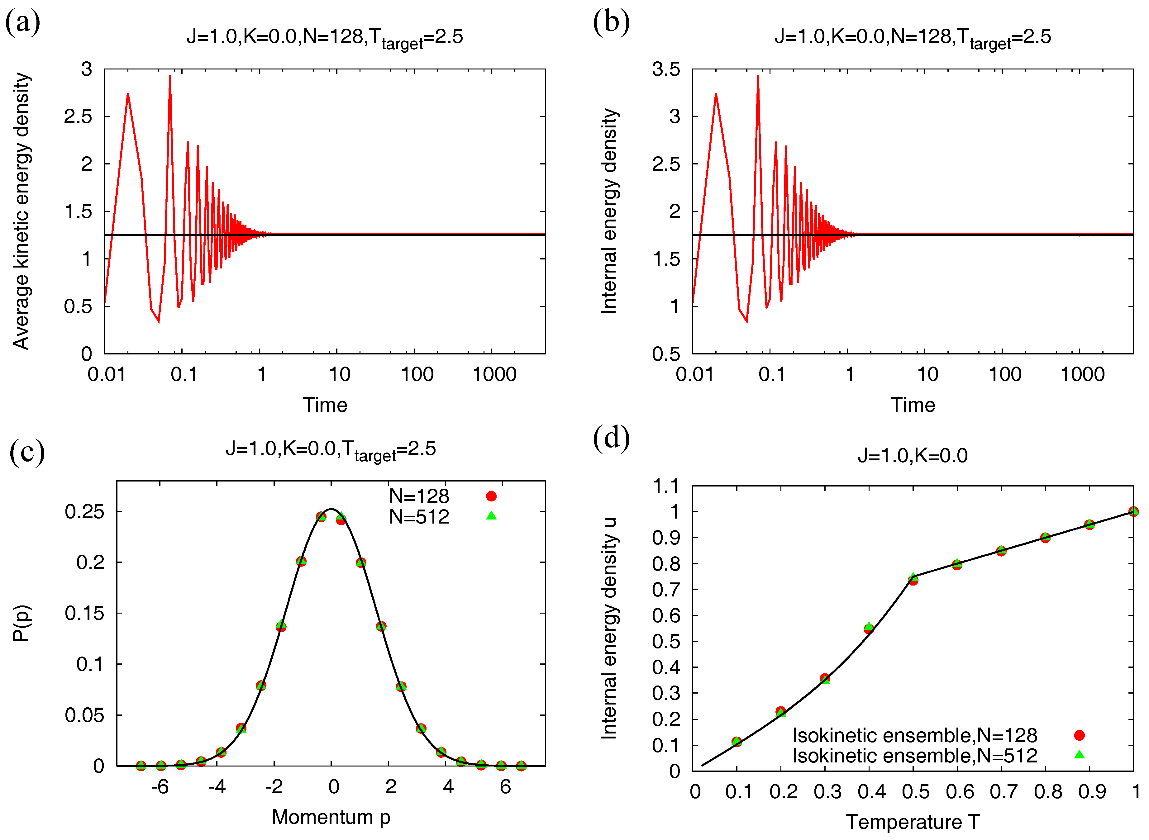
-spins occupying the sites of a one-dimensional periodic lattice and interacting via a long-range (specifically, a mean–field interaction in which every spin interacts with every other and a short-range (specifically, a nearest-neighbor interaction in which every spin interacts with its left and right neighbors) interaction. With an aim to study the equilibrium properties as well as relaxation towards equilibrium, we simulate the Nosé–Hoover dynamics of the model by integrating the corresponding equations of motion in time. A signature of canonical equilibrium is a single-particle momentum distribution that is Gaussian (see Equation (
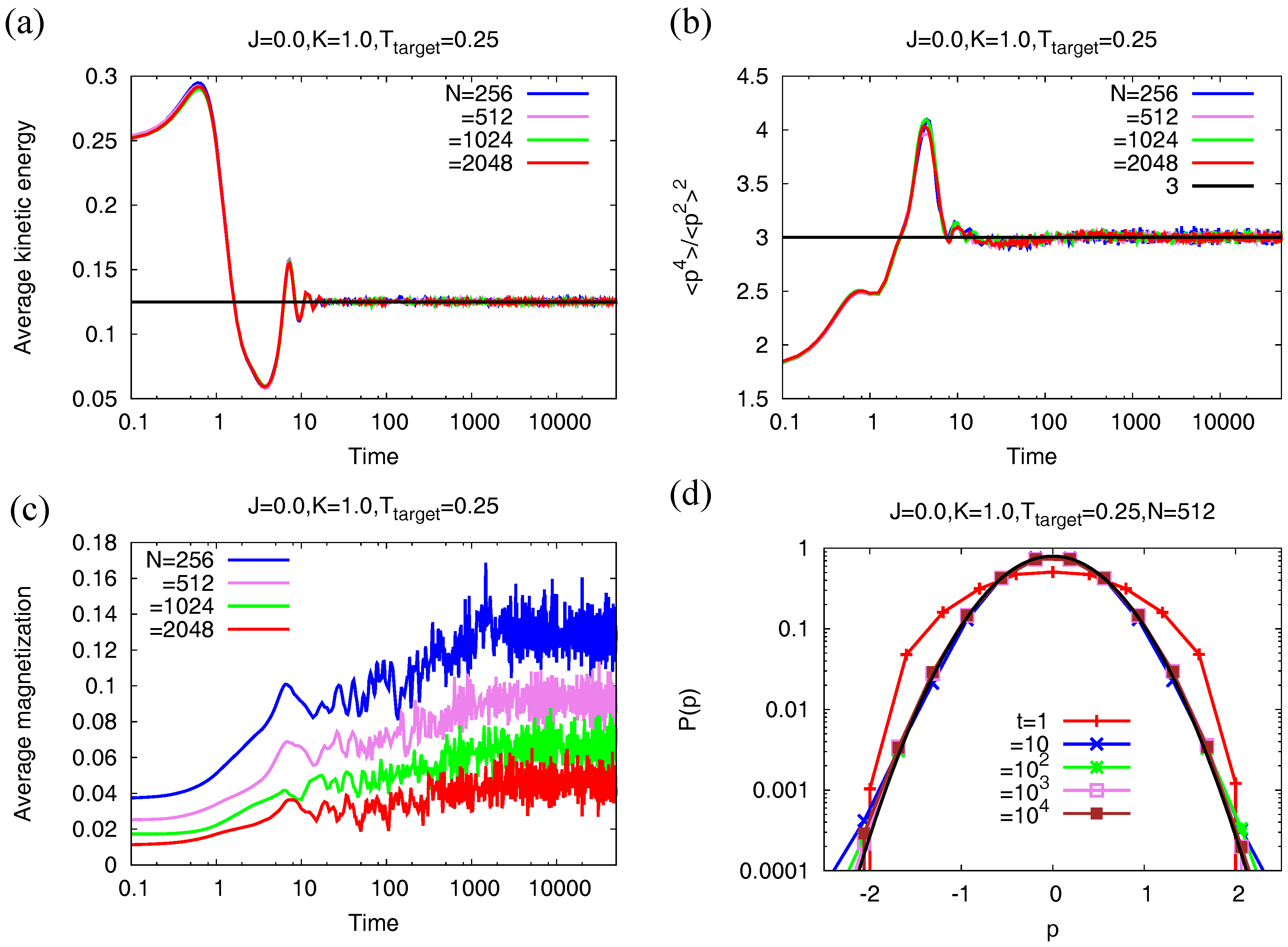
17)). We find that the equilibrium properties of our model system evolving under the Nosé–Hoover dynamics coincide with those within the canonical ensemble. As regards relaxation towards canonical equilibrium, we observe that starting from out-of-equilibrium initial conditions, the average kinetic energy of the system relaxes to its target canonical-equilibrium value over a
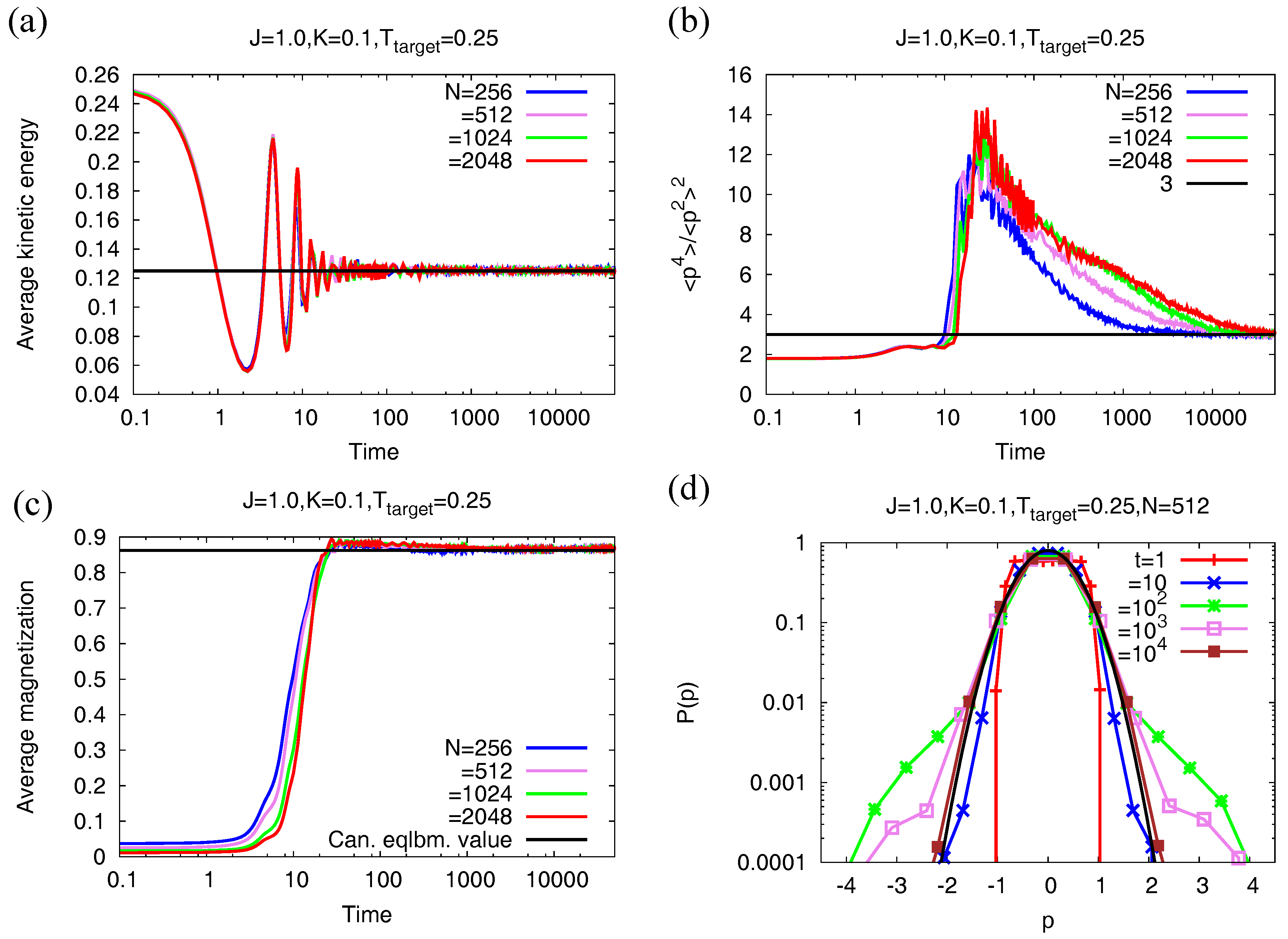
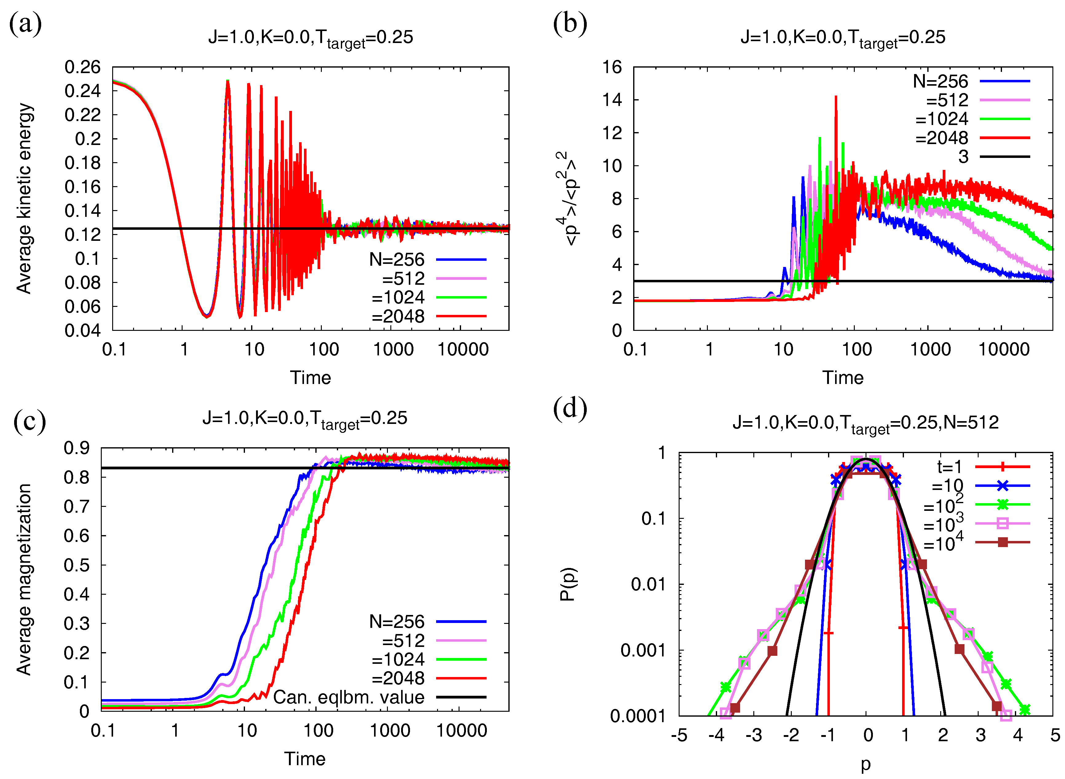
size-independent timescale. However, quite surprisingly, our results indicate that under the same conditions and with only long-range interactions present in the system, the momentum distribution relaxes to its Gaussian form in equilibrium over a scale that
diverges with the system size. On adding short-range interactions, the relaxation is found to occur over a timescale that has a much weaker dependence on system size. This system-size dependence vanishes when only short-range interactions are present in the system. An implication of such an ultra-slow relaxation when only long-range interactions are present in the system is that macroscopic observables other than the average kinetic energy when estimated in the Nosé–Hoover dynamics may take an unusually long time to relax to its canonical equilibrium value. Our work underlines the crucial role that interactions play in deciding the equivalence between Nosé–Hoover and canonical equilibrium.
The paper is organized as follows. In
Section 2, we describe the model of study. In
Section 3, we obtain the so-called caloric curve of the model within the canonical ensemble, which we eventually invoke in later parts of the paper to decide on the equivalence of the equilibrium properties of the Nosé–Hoover dynamics and canonical equilibrium. In
Section 4, we present results from simulations of the Nosé–Hoover dynamics of the model, and discuss the implications and relevance of the results. The paper ends with conclusions in
Section 5.
2. Model of Study
Our system of study comprises a one-dimensional periodic lattice of
N sites. Each site of the lattice is occupied by a unit-inertia rotor characterized by its angular coordinate
and the corresponding conjugated momentum
, with
. One may also think of the rotors as representing classical
-spins. Note that both of the
’s and the
’s are one-dimensional variables. There exist both a long-range (specifically, a global or a mean–field) coupling and a short-range (specifically, nearest-neighbor) coupling between the rotors. Thus, a rotor on site
j interacts with strength
with rotors on all the other sites and with strength
K with the rotor occupying the
-th and the
-th site. The Hamiltonian of the system is given by [
13,
14]
Note that, for
, the Hamiltonian (
18) reduces to that of the widely-studied Hamiltonian mean–field (HMF) model [
15], which is regarded as a paradigmatic model to study statics and dynamics of LRI systems [
10]. On the other hand, for
, the model (
18) reduces to a short-ranged
model in one dimension.
In the following, we take both the mean–field coupling J and the short-range coupling K to be positive, thereby modeling ferromagnetic global and nearest-neighbor couplings. Consequently, both the long-range and the short-range coupling between the rotors favor an ordered state in which all the rotor angles are equal, thereby minimizing the potential energy contribution to the total energy. Such a tendency is, however, opposed by the kinetic energy contribution whose average in equilibrium may be characterized by a temperature by invoking the Theorem of Equipartition. Noting that, for a given N, the total potential energy is bounded from above while the total kinetic energy is not, one expects the system to show in equilibrium an ordered/magnetized phase at low energies/temperatures and a disordered/unmagnetized phase at high energies/temperatures. This scenario holds even with .
The amount of order in the system is characterized by the
magnetization
which is a vector whose length
m has the thermodynamic value in equilibrium denoted by
that is nonzero in the ordered phase and zero in the disordered phase. For
, the corresponding HMF model is known to display a second-order phase transition between a high-temperature unmagnetized phase and a low-temperature magnetized phase at the critical temperature
, with the corresponding critical energy density being
[
10]. On the other hand, invoking the Landau’s argument for the absence of any phase transition at a finite temperature in a one-dimensional model with only short-range interactions, one may conclude for
that the corresponding short-ranged
model does not display any phase transitions, though it has been shown to have interesting dynamical effects [
16]. For general
, when both long-range and short-range interactions are present, the model displays a second-order phase transition between an ordered and a disordered phase [
13,
14]. Note that all the mentioned phase transitions are continuous. Although ensemble equivalence is not guaranteed for LRI systems, it has been argued that inequivalence arises when one has a first-order phase transition in the canonical ensemble, and not when one has a second-order transition [
17]. Consequently, we may regard the phase diagram of model (
18) to be equivalent within microcanonical and canonical ensembles. For an explicit demonstration of ensemble equivalence for the model (
18), one may refer to [
14].
In the following section, we will obtain the caloric curve of model (
18) that relates the equilibrium internal energy with the equilibrium temperature of the system.
5. Conclusions
In this paper, we investigated the relaxation properties of the Nosé–Hoover dynamics of many-body interacting Hamiltonian systems, with an emphasis on the effect of inter-particle interactions. The dynamics aim to generate the canonical equilibrium distribution of a system at the desired temperature by employing time-reversible, deterministic dynamics. To pursue our study, we considered a representative model comprising N classical -spins occupying the sites of a one-dimensional periodic lattice. The spins interact with one another via both a long-range interaction, modelled as a mean–field interaction in which every spin interacts with every other, and a short-range one, modelled as a nearest-neighbor interaction in which every spin interacts with its left and right neighboring spins. We studied the Nosé–Hoover dynamics of the model through N-body integration of the corresponding equations of motion. Canonical equilibrium is characterized by a momentum distribution that is Gaussian. We found that the equilibrium properties of our model system evolving according to Nosé–Hoover dynamics are in excellent agreement with exact analytic results for the equilibrium properties derived within the canonical ensemble. Moreover, while starting from out-of-equilibrium initial conditions, the average kinetic energy of the system relaxes to its target value over a size-independent timescale. However, quite unexpectedly, we found that under the same conditions and with only long-range interactions present in the system, the momentum distribution relaxes to its Gaussian form in equilibrium over a scale that grows with N. The N-dependence gets weaker on adding short-range interactions, and vanishes when the latter are the only inter-particle interactions present in the system.
Viewed from the perspective of LRI systems, the slow relaxation observed within the Nosé–Hoover dynamics allows for drawing an analogy with a similar slow relaxation observed within the microcanonical dynamics of isolated LRI systems, a phenomenon that leads to the occurrence of nonequilibrium quasistationary states (QSSs) that have lifetimes diverging with the system size [
10,
21]. Within a kinetic theory approach, the QSSs are understood as stable, stationary solutions of the so-called Vlasov equation that governs the time evolution of the single-particle phase space distribution. The Vlasov equation is obtained as the first equation of the Bogoliubov–Born–Green–Yvon–Kirkwood (BBGKY) hierarchy by neglecting the correlation between particle trajectories, with corrections that decrease with an increase of
N. For large but finite
N, the eventual relaxation of QSSs towards equilibrium is understood as arising due to these finite-
N corrections, the so-called collisional terms, to the Vlasov equation. In models in which the momentum variables are one-dimensional, it has been shown by analyzing the behavior of the dominant collisional term that Vlasov-stable phase-space distributions that are homogeneous in the coordinates evolve on times much larger than
N, thereby leading for the distributions to characterize QSSs that have lifetimes diverging with
N [
8,
11,
22]. In light of the foregoing discussions, it is evidently pertinent and of immediate interest to invoke a kinetic theory approach and investigate in the context of the Nosé–Hoover dynamics of long-range systems whether additional short-range interactions play the role of collisional dynamics that speed up the relaxation of the system towards canonical equilibrium. Work in this direction is in progress and will be reported elsewhere.
The agreement reported in this paper in the value of the average kinetic energy computed in canonical equilibrium and within the Nosé–Hoover dynamics is reminiscent of a similar agreement in the large-system limit between ensemble and time averages predicted by Khinchin for the so-called sum-functions, that is, functions such as the kinetic energy that are sums of single-particle contributions [
23]. The result was obtained for rarefied gases, which was later observed to also hold for systems with short-range interactions [
24,
25]. Our work hints at the validity of such a result even for long-range systems, as is evident from the agreement in the value of the average kinetic energy computed within the Nosé–Hoover dynamics and in canonical equilibrium (see
Figure 4a). This point warrants a more detailed investigation that will be left for future studies.


