
Local Entropy Generation in Compressible Flow through a High Pressure Turbine with Delayed Detached Eddy Simulation

Abstract
:1. Introduction
2. Review of an Experimental Test Rig
3. Numerical Methods
3.1. Governing Equations
3.2. Turbulence Model
3.3. Delayed Detached Eddy Simulation
3.4. Low-Dissipation Numerical Scheme
3.5. Entropy Generation Rate
3.5.1. Viscous Losses and Thermal Losses
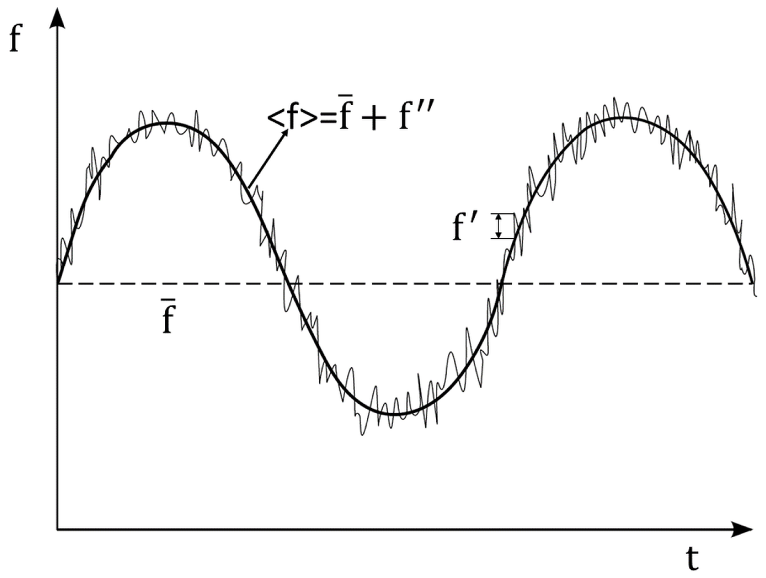
3.5.2. Losses Due to Steady Effects and Unsteady Effects
3.5.3. Discussion of the Losses Obtained by Different Simulation Methods
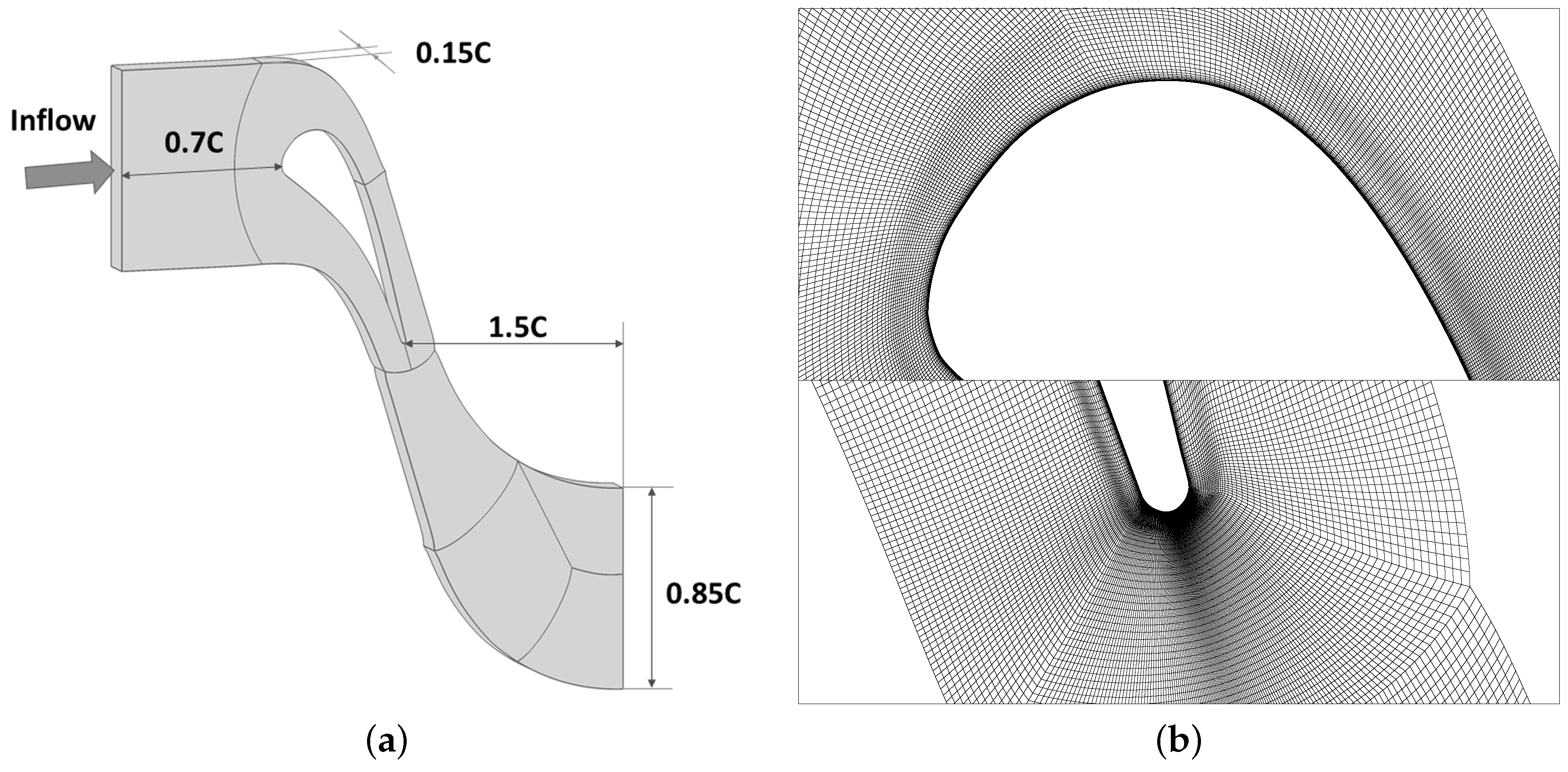
4. Computational Setup
5. Results and Discussions
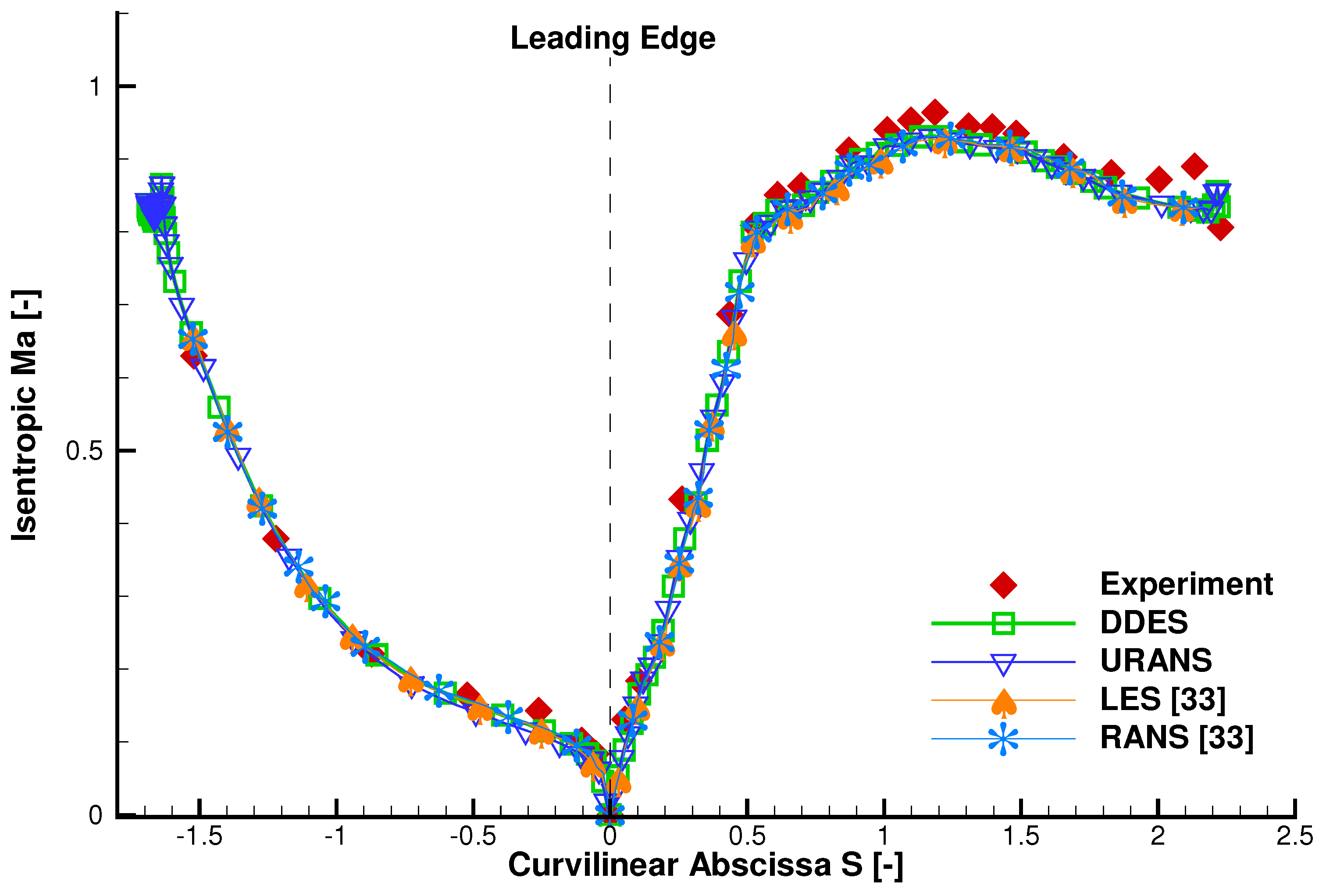
5.1. Validation and Comparison of the Results
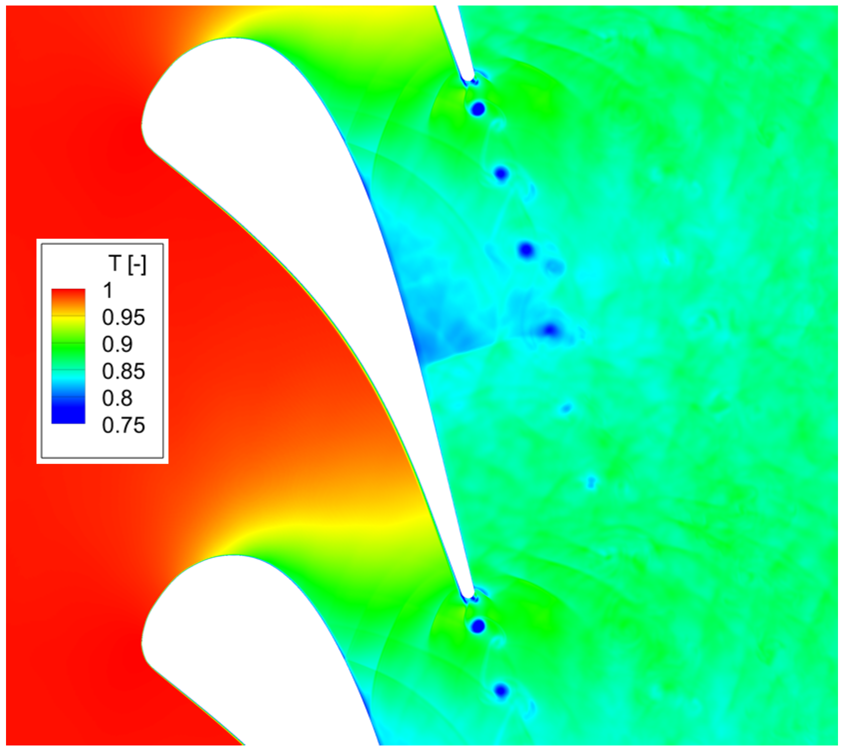
5.2. Flow Field in a High Pressure Turbine Vane Passage
5.3. Loss Analysis
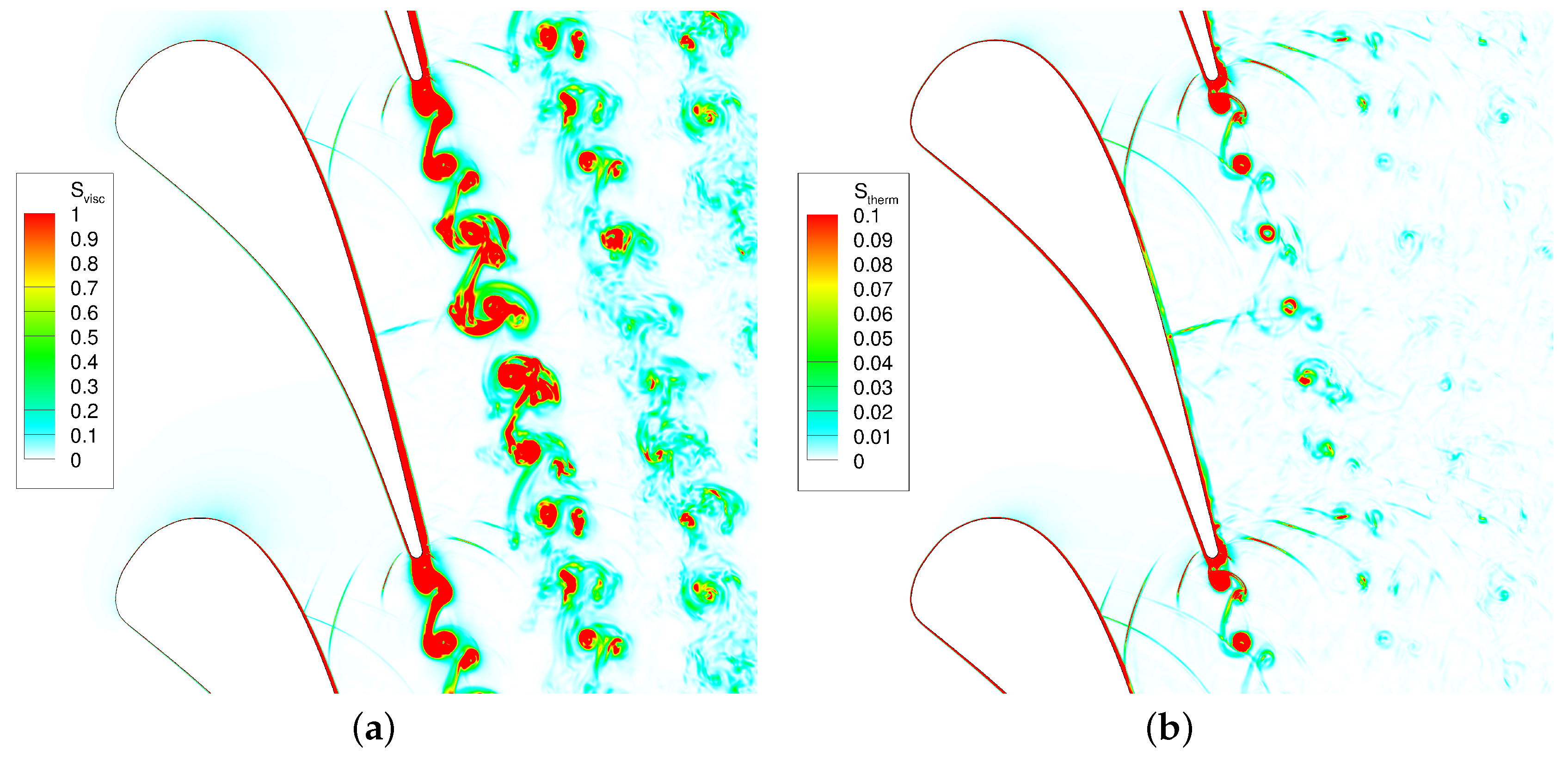
5.3.1. Viscous Losses and Thermal Losses
5.3.2. Losses Due to Steady and Unsteady Effects
5.3.3. Loss Analysis in the Wake Area
6. Conclusions
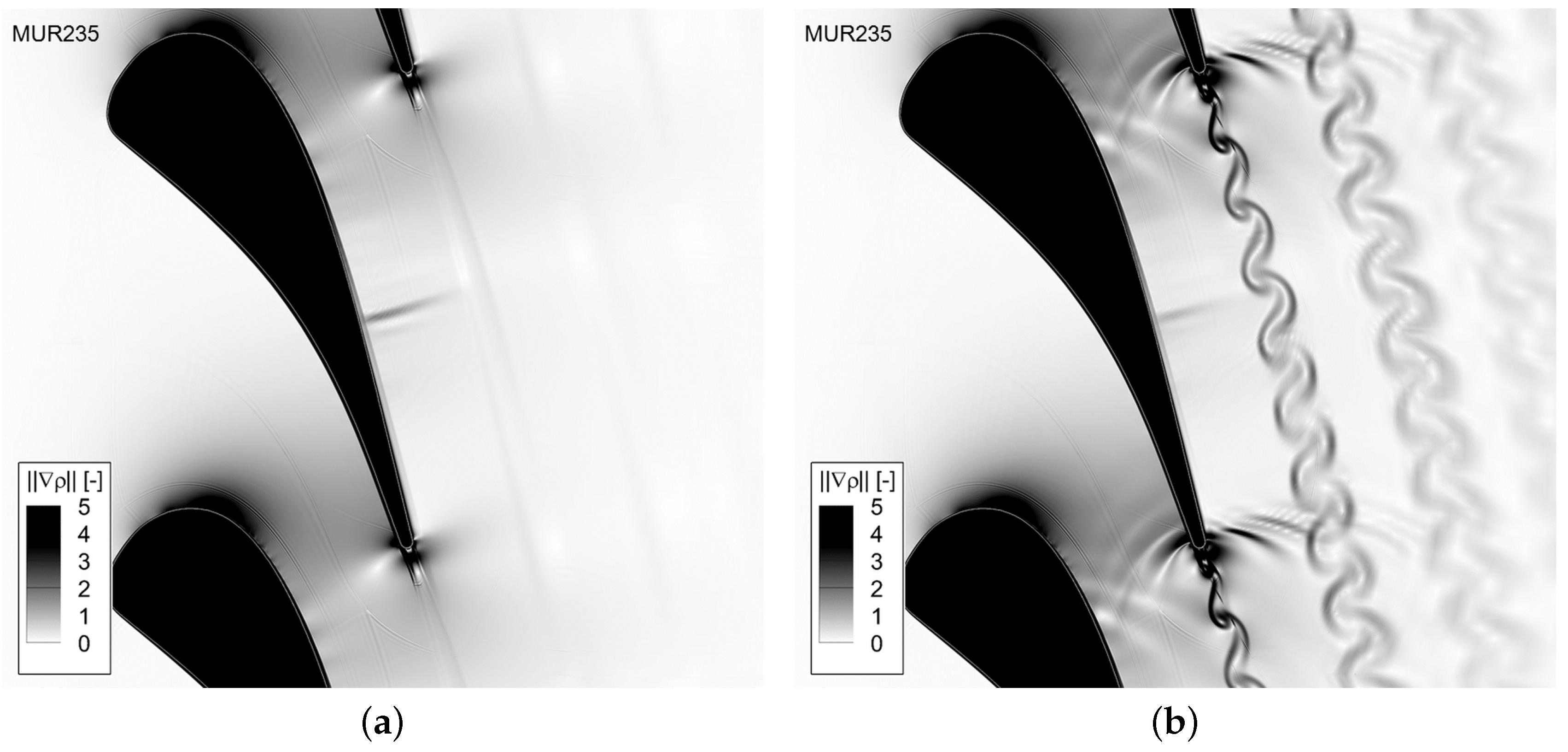
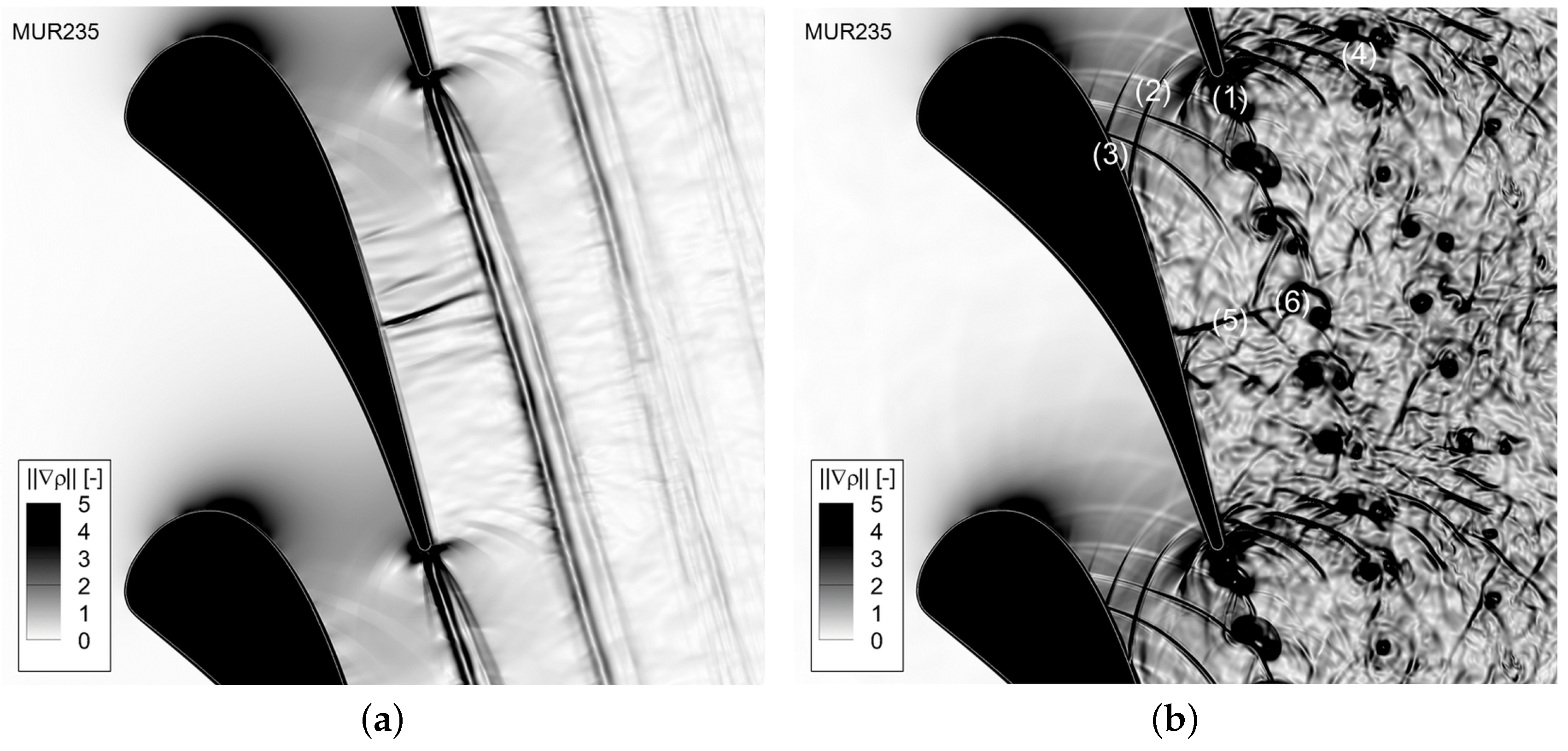
- The accuracy of flow modeling and details of flow structures are the cornerstone of accurate local loss analysis. URANS fails to accurately capture the length characteristics of the wake vortex due to its incapability in modeling such flow. DDES can accurately produce the flow structures with abundant details that are comparable to LES results. The DDES method is validated by several previous experimental findings. This establishes a solid foundation of accurate losses prediction. The local loss analysis based on DDES is more reliable than that based on URANS for complex flows inside the high-pressure turbine vane.
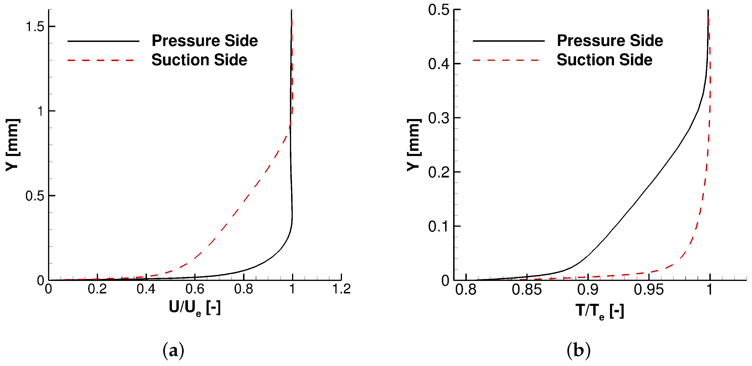
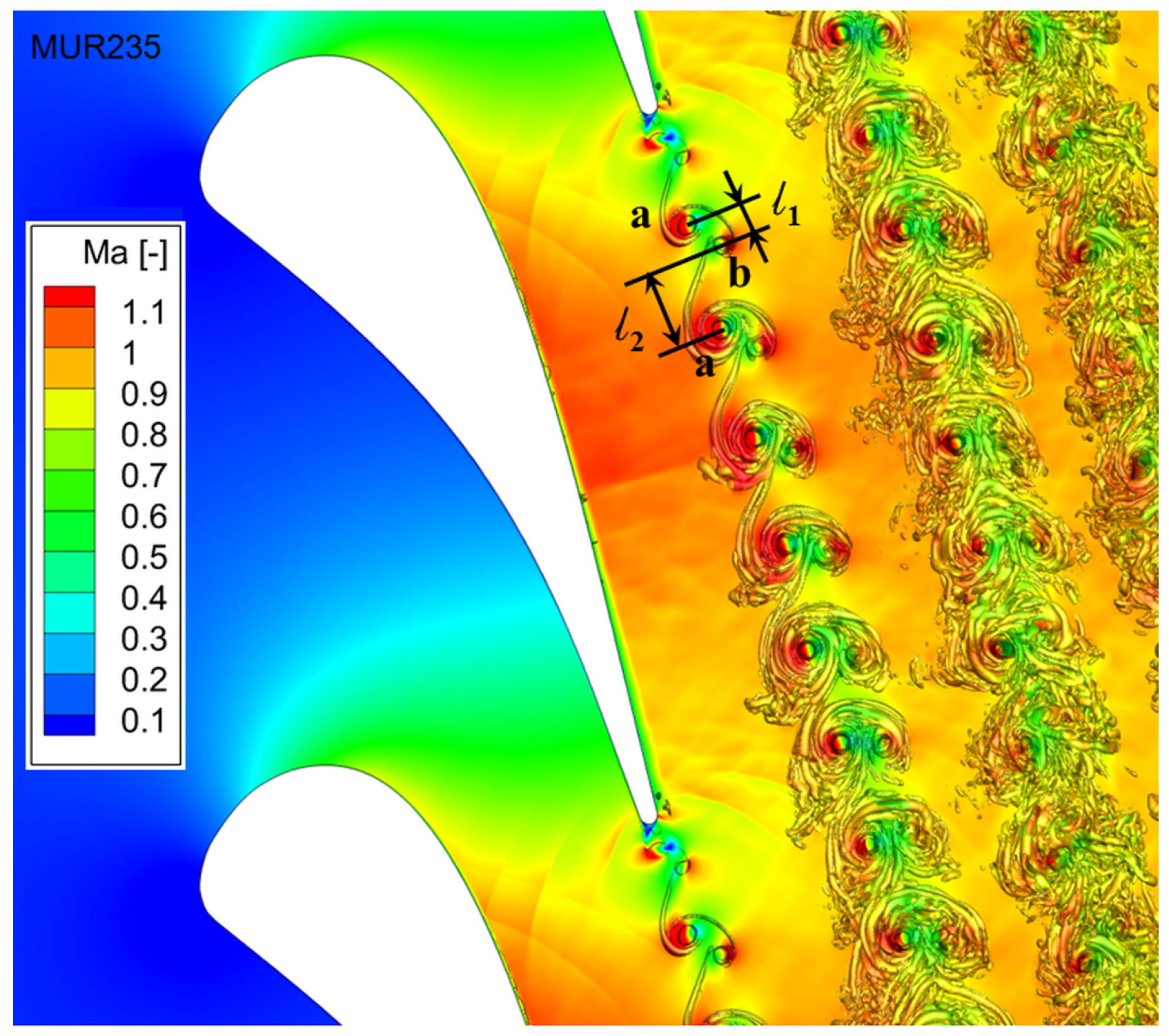
- In the high-pressure turbine vane, the viscous irreversibility is the main contributor to the total losses, while the heat transfer irreversibility accounts for less than 10% for both instantaneous and time-averaged field. The boundary layer, wake vortex, shock wave and pressure waves give rise to high losses. The suction side of the vane has a thicker high layer than the pressure side because the suction side has a thicker momentum boundary than the pressure side, while the high layers over the two sides have comparable thickness resulting from similar temperature boundary layer thicknesses. The wake vortex is the main origin of both unsteadiness and losses.
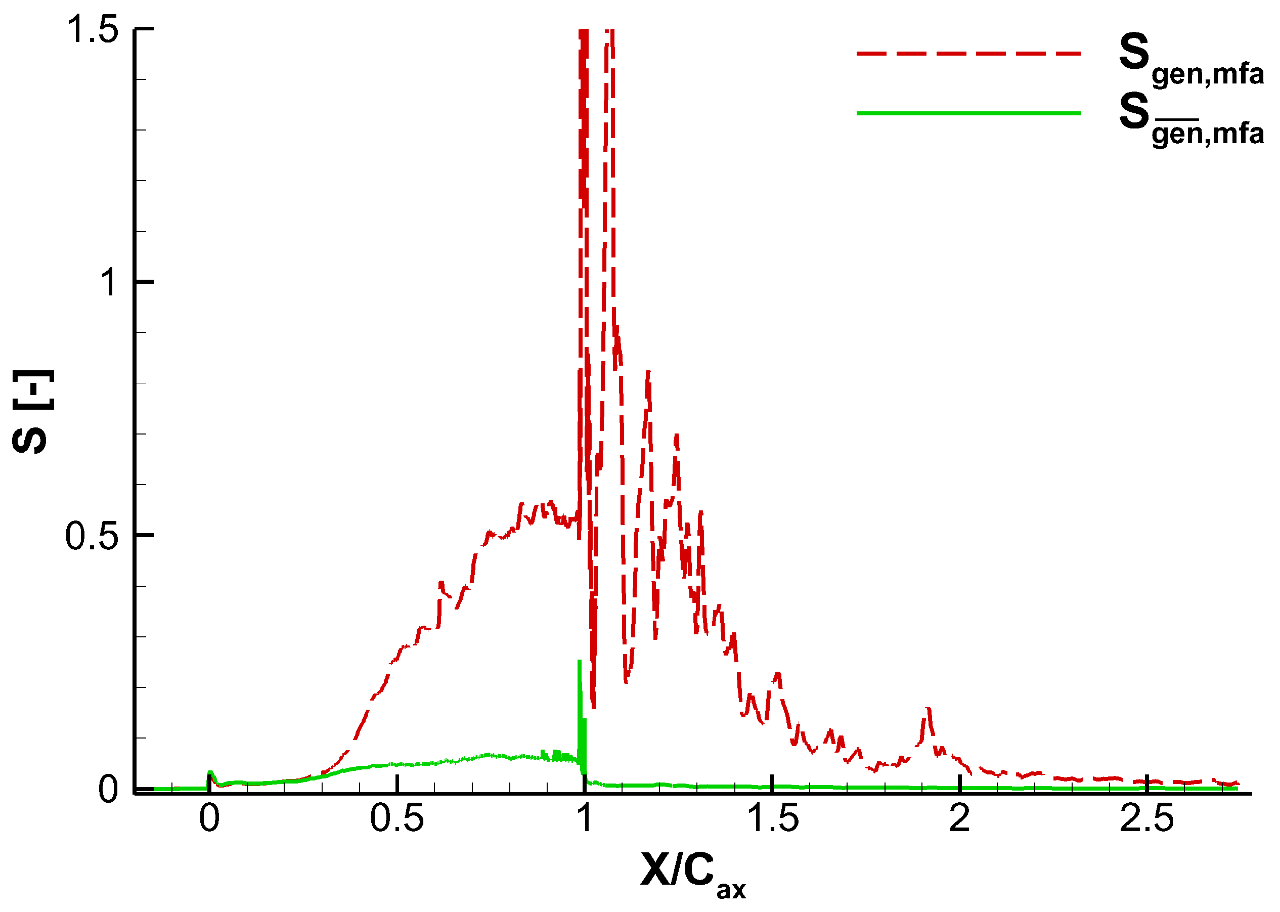
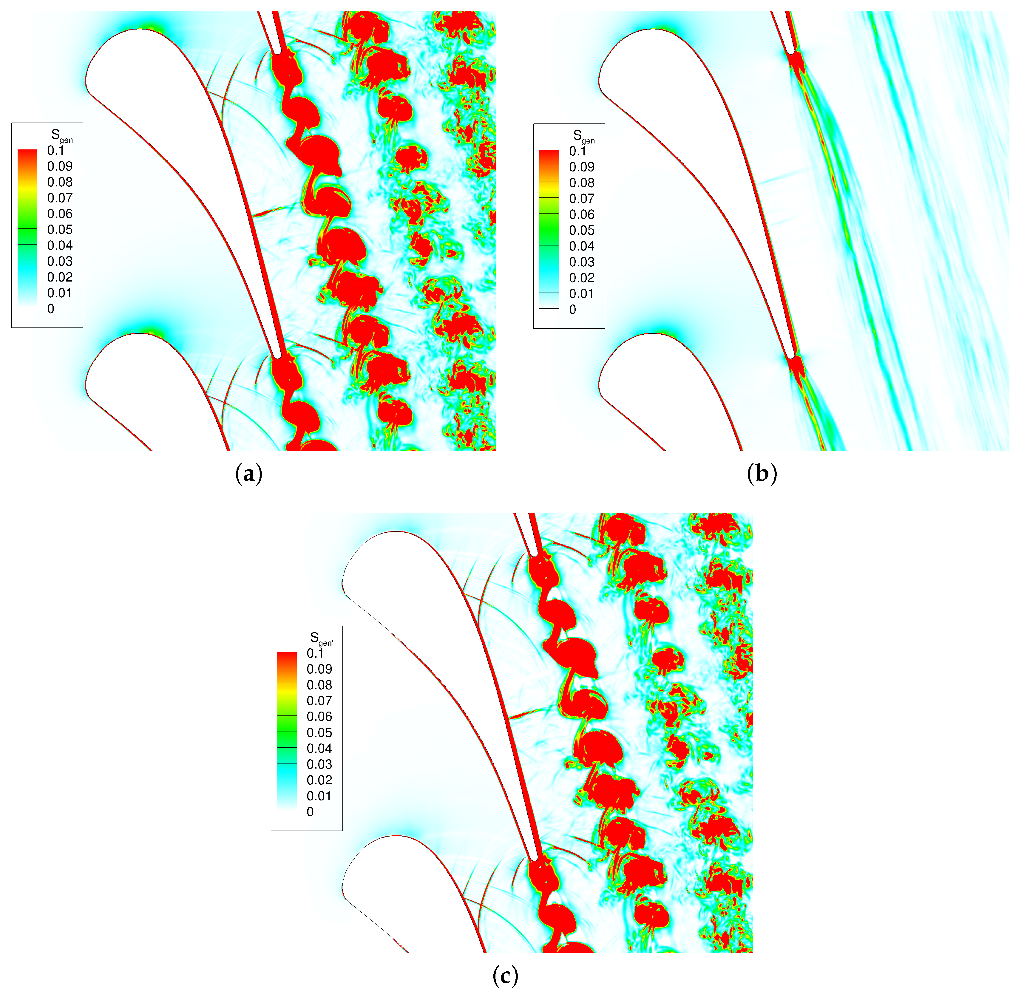
- Losses due to unsteady effects are much higher than that due to steady effects. The unsteadiness propagates upstream by the pressure waves and downstream by the motion of the vortex. The unsteadiness in the flow passage is with different strengths at different positions. The unsteadiness before the axial position is not significant and becomes very strong in the rear part of the vane and downstream of the trailing edge. This points out that the unsteady effects are very important and should not be omitted in the design system.
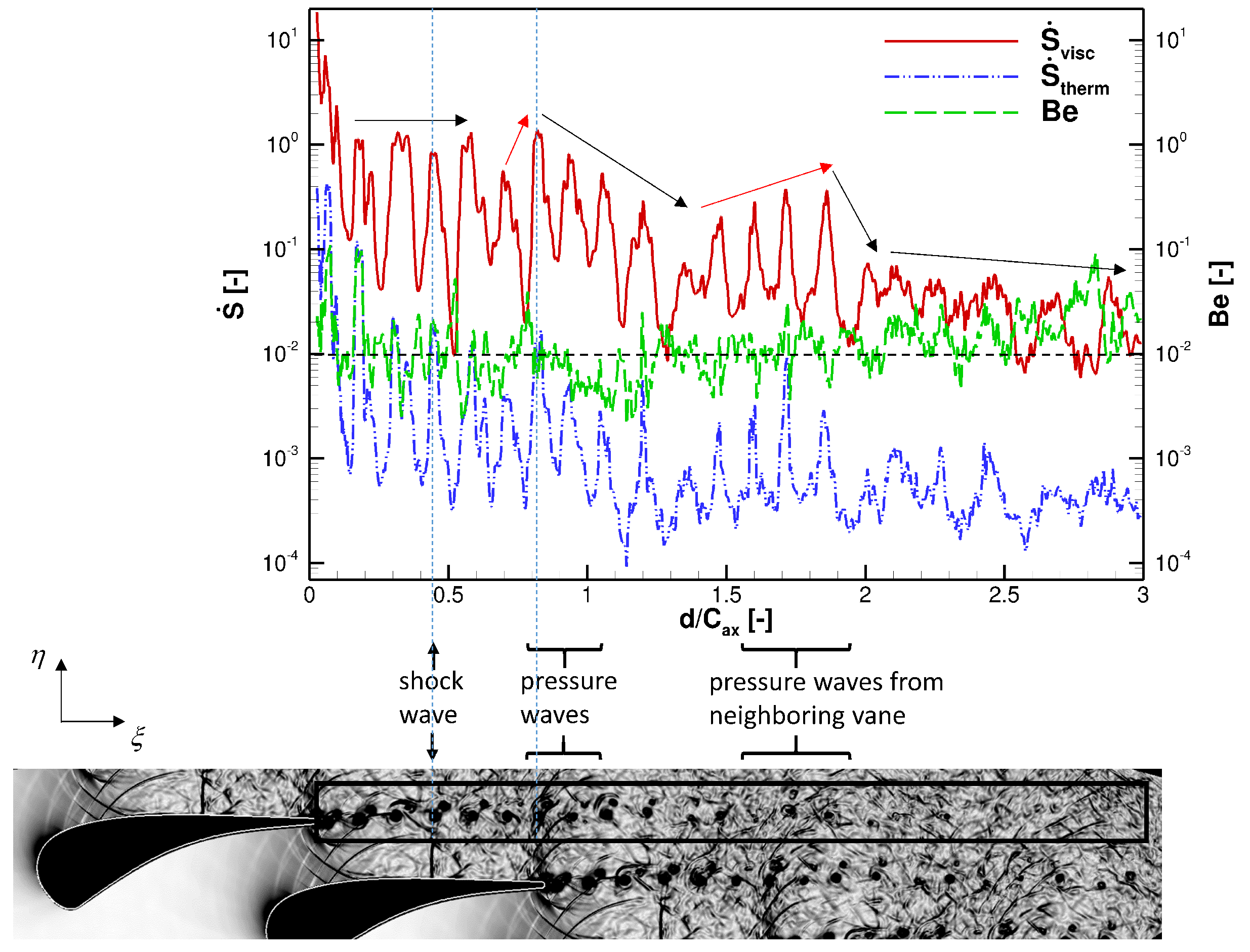
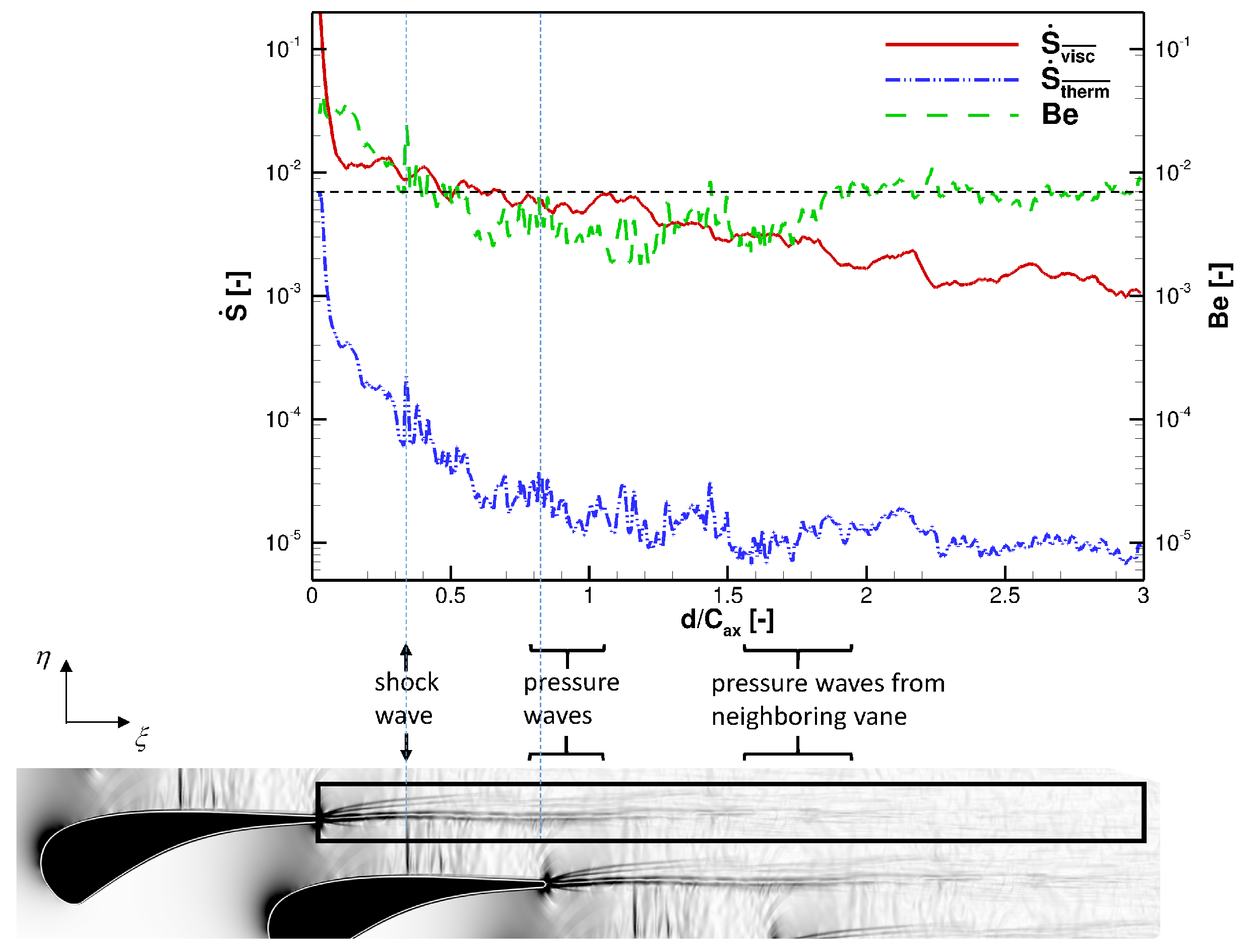
- The entropy generation rate analysis in the wake area also finds that the interaction between the wake vortex and pressure waves is stronger than the interaction between the wake vortex and shock wave in terms of loss generation. In the wake region, the thermal irreversibility and the viscous reversibility decrease at slightly different speeds. In general, thermal and viscous losses in the wake region have positive correlation, and this is good for losses reduction since they can be reduced simultaneously.
Acknowledgments
Author Contributions
Conflicts of Interest
Nomenclature
| Be | Bejan number |
| C | chord, stagnation pressure loss coefficient |
| f | any flow variable |
| h | enthalpy |
| k | thermal conductivity |
| Ma | Mach number |
| P | pressure |
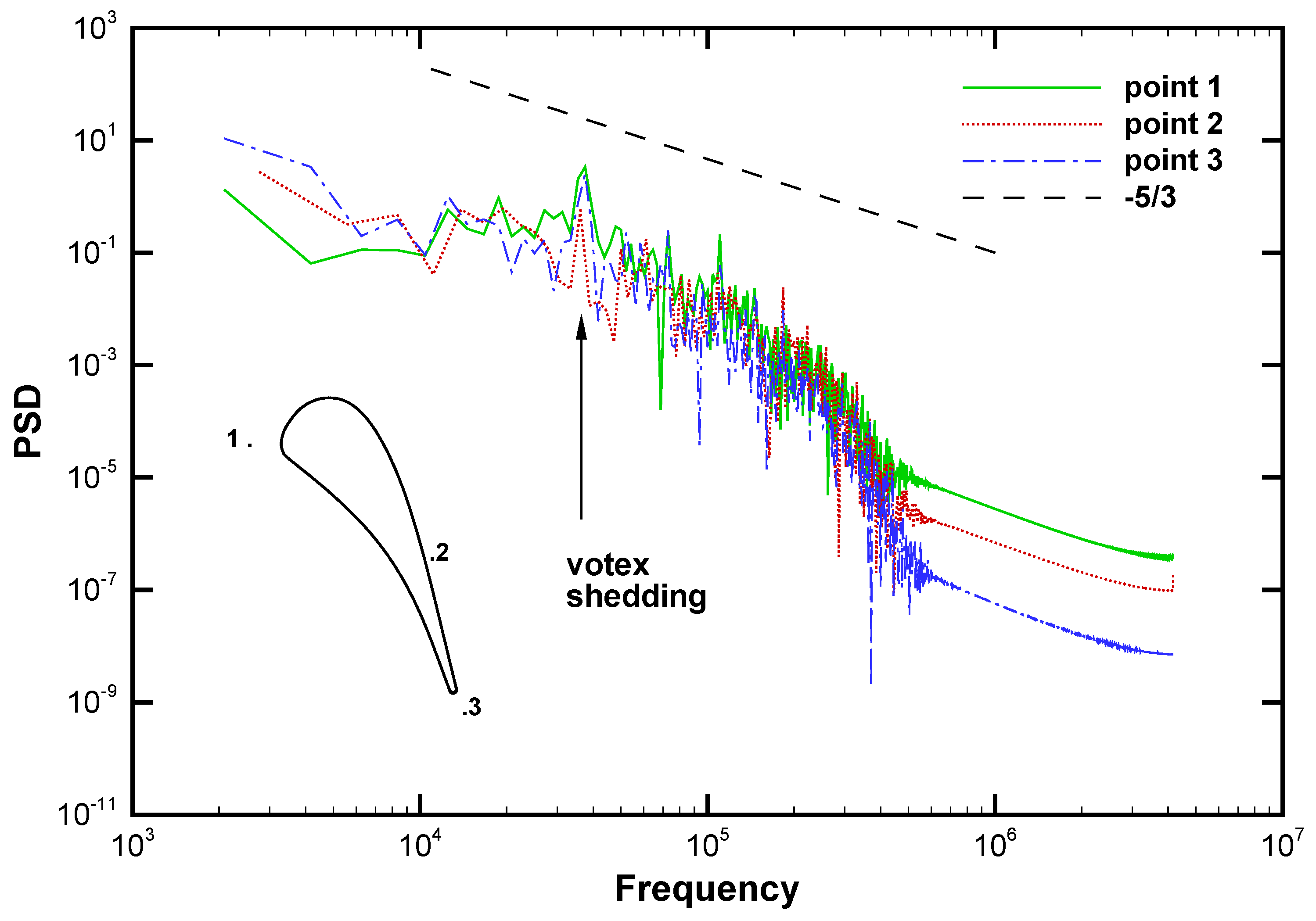
| PSD | power spectral density |
| R | gas constant |
| r | radius, mixing length |
| Re | Reynolds number |
| S | mean strain, curvilinear abscissa |
| s | entropy |
| T | temperature |
| τ0 | characteristic convective time |
| u | axial velocity |
| v | tangential velocity |
| w | span-wise velocity |
Greek Letters
| τ | viscous stress tensor |
| κ | von Karman constant |
| μ | viscosity |
| ν | kinematic viscosity |
| ρ | density |
| Ω | rotation rate, vorticity |
| ζ | loss coefficient |
Subscripts
| is | isentropic |
| ax | axial |
| inl | inlet |
| LE | leading edge |
| mfa | mass flow averaged variables |
| out | outlet |
| TE | trailing edge |
| ref | reference condition |
| t | turbulent |
| vortex | vortex shedding |
| wall | wall |
Superscripts
| * | total |
References
- Padurean, A.; Cormos, C.C.; Agachi, P.S. Pre-combustion carbon dioxide capture by gas–liquid absorption for integrated gasification combined cycle power plants. Int. J. Greenh. Gas Control 2012, 7, 1–11. [Google Scholar] [CrossRef]
- Brown, L. Axial flow compressor and turbine loss coefficients: A comparison of several parameters. J. Eng. Power 1972, 94, 193–201. [Google Scholar] [CrossRef]
- Denton, J.D. Loss mechanisms in turbomachines. In Proceedings of the ASME 1993 International Gas Turbine and Aeroengine Congress and Exposition, Cincinnati, OH, USA, 24–27 May 1993; p. V002T14A001.
- Winterbone, D.; Turan, A. Advanced Thermodynamics for Engineers; Butterworth-Heinemann: Oxford, UK, 2015. [Google Scholar]
- Dixon, S.L.; Hall, C. Fluid Mechanics and Thermodynamics of Turbomachinery; Butterworth-Heinemann: Oxford, UK, 2013. [Google Scholar]
- Moran, M.J.; Shapiro, H.N.; Boettner, D.D.; Bailey, M.B. Fundamentals of Engineering Thermodynamics; John Wiley & Sons: Hoboken, NJ, USA, 2010. [Google Scholar]
- Herwig, H.; Schmandt, B. How to determine losses in a flow field: A paradigm shift towards the second law analysis. Entropy 2014, 16, 2959–2989. [Google Scholar] [CrossRef]
- Bejan, A. A study of entropy generation in fundamental convective heat transfer. J. Heat Trans. 1979, 101, 718–725. [Google Scholar] [CrossRef]
- Ko, T.; Ting, K. Entropy generation and optimal analysis for laminar forced convection in curved rectangular ducts: A numerical study. Int. J. Therm. Sci. 2006, 45, 138–150. [Google Scholar] [CrossRef]
- Yapici, H.; Kayatas, N.; Kahraman, N.; Bastürk, G. Numerical study on local entropy generation in compressible flow through a suddenly expanding pipe. Entropy 2005, 7, 38–67. [Google Scholar] [CrossRef]
- Adeyinka, O.; Naterer, G. Entropy-based metric for component-level energy management: Application to diffuser performance. Int. J. Energy Res. 2005, 29, 1007–1024. [Google Scholar] [CrossRef]
- Hassan, M.; Sadri, R.; Ahmadi, G.; Dahari, M.B.; Kazi, S.N.; Safaei, M.R.; Sadeghinezhad, E. Numerical study of entropy generation in a flowing nanofluid used in micro-and minichannels. Entropy 2013, 15, 144–155. [Google Scholar] [CrossRef]
- Denton, J.; Pullan, G. A numerical investigation into the sources of endwall loss in axial flow turbines. In Proceedings of the ASME Turbo Expo 2012: Turbine Technical Conference and Exposition, Copenhagen, Denmark, 11–15 June 2012; pp. 1417–1430.
- Zlatinov, M.B.; Tan, C.S.; Montgomery, M.; Islam, T.; Harris, M. Turbine hub and shroud sealing flow loss mechanisms. J. Turbomach. 2012, 134, 061027. [Google Scholar] [CrossRef]
- Jin, Y.; Herwig, H. From single obstacles to wall roughness: Some fundamental investigations based on DNS results for turbulent channel flow. Z. Angew. Math. Phys. 2013, 64, 1337–1351. [Google Scholar] [CrossRef]
- Jin, Y.; Herwig, H. Turbulent flow and heat transfer in channels with shark skin surfaces: Entropy generation and its physical significance. Int. J. Heat Mass Transf. 2014, 70, 10–22. [Google Scholar] [CrossRef]
- Tucker, P.G. Computation of unsteady turbomachinery flows: Part 1–Progress and challenges. Prog. Aerosp. Sci. 2011, 47, 522–545. [Google Scholar] [CrossRef]
- Im, H.S.; Zha, G.C. Delayed detached eddy simulation of airfoil stall flows using high-order schemes. J. Fluids Eng. 2014, 136, 111104. [Google Scholar] [CrossRef]
- Tucker, P.G. Computation of unsteady turbomachinery flows: Part 2—LES and hybrids. Prog. Aerosp. Sci. 2011, 47, 546–569. [Google Scholar] [CrossRef]
- Kopriva, J.E.; Laskowski, G.M.; Sheikhi, M.R.H. Computational assessment of inlet turbulence on boundary layer development and momentum/thermal wakes for high pressure turbine nozzle and blade. In Proceedings of the ASME 2014 International Mechanical Engineering Congress and Exposition, Montreal, QC, Canada, 14–20 November 2014; p. V08BT10A006.
- Spalart, P.; Jou, W.; Strelets, M.; Allmaras, S. Comments on the feasibility of LES for wings, and on a hybrid RANS/LES approach. Adv. DNS/LES 1997, 1, 4–8. [Google Scholar]
- Bhaskaran, B. Large Eddy Simulation of High Pressure Trbine Cascade; Stanford University: Stanford, CA, USA, 2010. [Google Scholar]
- Laskowski, G.M.; Kopriva, J.; Michelassi, V.; Shankaran, S.; Paliath, U.; Bhaskaran, R.; Wang, Q.; Talnikar, C.; Wang, Z.; Jia, F. Future directions of high-fidelity CFD for aero-thermal turbomachinery research, analysis and design. In Proceedings of the 46th AIAA Fluid Dynamics Conference, Washington, DC, USA, 13–17 June 2016.
- Sieverding, C. Sample calculations—Turbine tests. Transonic Flows Turbomach. 1973. [Google Scholar]
- Sieverding, C. Workshop on Two Dimensional and Three Dimensional Flow Calculations in Turbine Bladings. Numer. Meth. Flows Turbomach. Bladings 1982. [Google Scholar]
- Arts, T.; De Rouvroit, M.L.; Rutherford, A. Aero-thermal Investigation of A Highly Loaded Transonic Linear Turbine Guide Vane Cascade; von Karman Institute for Fluid Dynamics: Sint-Genesius-Rode, Belgium, 1990. [Google Scholar]
- Spalart, P.R.; Allmaras, S.R. A one equation turbulence model for aerodinamic flows. In Proceedings of the 30th Aerospace Sciences Meeting and Exhibit, Reno, NV, USA, 6–9 January 1992.
- Coronado, P.; Wang, B.; Zha, G.C. Delayed detached eddy simulation of shock wave/turbulent boundary layer interaction. In Proceedings of the 48th AIAA Aerospace Sciences Meeting Including the New Horizons Forum and Aerospace Exposition, Orlando, FL, USA, 4–7 January 2010; pp. 4–6.
- Spalart, P.R.; Deck, S.; Shur, M.; Squires, K.; Strelets, M.K.; Travin, A. A new version of detached-eddy simulation, resistant to ambiguous grid densities. Theor. Comput. Fluid Dyn. 2006, 20, 181–195. [Google Scholar] [CrossRef]
- Strelets, M. Detached eddy simulation of massively separated flows. In Proceedings of the 39th Aerospace Sciences Meeting and Exhibit, Reno, NV, USA, 8–11 January 2001.
- Liu, J.; Xiao, Z.; Fu, S. Unsteady flow around two tandem cylinders using advanced turbulence modeling method. In Computational Fluid Dynamics 2010; Springer: Berlin/Heidelberg, Germany, 2011; pp. 879–881. [Google Scholar]
- Roe, P.L. Approximate Riemann solvers, parameter vectors, and difference schemes. J. Comput. Phys. 1981, 43, 357–372. [Google Scholar] [CrossRef]
- Su, X.; Yamamoto, S.; Yuan, X. On the accurate prediction of tip vortex: Effect of numerical schemes. In Proceedings of the ASME Turbo Expo 2013: Turbine Technical Conference and Exposition, San Antonio, TX, USA, 3–7 June 2013; p. V06BT37A013.
- Su, X.; Sasaki, D.; Nakahashi, K. On the efficient application of Weighted Essentially Nonoscillatory scheme. Int. J. Numer. Meth. Fluids 2013, 71, 185–207. [Google Scholar] [CrossRef]
- Bejan, A. Entropy Generation through Heat and Fluid Flow; Wiley: New York, NY, USA, 1982. [Google Scholar]
- Morata, E.C.; Gourdain, N.; Duchaine, F.; Gicquel, L. Effects of free-stream turbulence on high pressure turbine blade heat transfer predicted by structured and unstructured LES. Int. J. Heat Mass Transf. 2012, 55, 5754–5768. [Google Scholar] [CrossRef]
- Cicatelli, G.; Sieverding, C. A review of the research on unsteady turbine blade wake characteristics. In Proceedings of the Loss Mechanisms and Unsteady Flows in Turbomachines, Propulsion and Energetics Panel 85th Symposium, Derby, UK, 8–12 May 1995.
- Sieverding, C.H.; Ottolia, D.; Bagnera, C.; Cimadoro, A.; Desse, J.M. Unsteady turbine blade wake characteristics. In Proceedings of the ASME Turbo Expo 2003, collocated with the 2003 International Joint Power Generation Conference, Atlanta, GA, USA, 16–19 June 2003; pp. 1081–1092.


| Parameter | Unit | Value |
|---|---|---|
| Chord length | (mm) | 67.647 |
| Pitch to chord ratio | (-) | 0.85 |
| Throat to chord ratio | (-) | 0.2207 |
| Flow inlet angle | (degree) | 0 |
| Stagger angle | (degree) | 55.0 (from axial direction) |
| (-) | 0.061 | |
| (-) | 0.0105 |
| Parameter | Unit | Case MUR129 | Case MUR235 |
|---|---|---|---|
| (-) | 0.840 | 0.927 | |
| (Pa) | 184900 | 182800 | |
| (Pa) | 116500 | 104900 | |
| (K) | 409.2 | 413.3 | |
| (K) | 298 | 301 |
© 2017 by the authors; licensee MDPI, Basel, Switzerland. This article is an open access article distributed under the terms and conditions of the Creative Commons Attribution (CC-BY) license (http://creativecommons.org/licenses/by/4.0/).
Share and Cite
Lin, D.; Yuan, X.; Su, X. Local Entropy Generation in Compressible Flow through a High Pressure Turbine with Delayed Detached Eddy Simulation. Entropy 2017, 19, 29. https://doi.org/10.3390/e19010029
Lin D, Yuan X, Su X. Local Entropy Generation in Compressible Flow through a High Pressure Turbine with Delayed Detached Eddy Simulation. Entropy. 2017; 19(1):29. https://doi.org/10.3390/e19010029
Chicago/Turabian StyleLin, Dun, Xin Yuan, and Xinrong Su. 2017. "Local Entropy Generation in Compressible Flow through a High Pressure Turbine with Delayed Detached Eddy Simulation" Entropy 19, no. 1: 29. https://doi.org/10.3390/e19010029
APA StyleLin, D., Yuan, X., & Su, X. (2017). Local Entropy Generation in Compressible Flow through a High Pressure Turbine with Delayed Detached Eddy Simulation. Entropy, 19(1), 29. https://doi.org/10.3390/e19010029