Article

An Urban Cellular Automata Model for Simulating Dynamic States on a Local Scale

Urban Planning, School of Architecture, Tampere University of Technology, Korkeakoulunkatu 5, Tampere 33720, Finland
Entropy 2017, 19(1), 12; https://doi.org/10.3390/e19010012
Submission received: 30 September 2016 / Revised: 13 December 2016 / Accepted: 20 December 2016 / Published: 28 December 2016
(This article belongs to the Special Issue Entropy for Sustainable and Resilient Urban Future)

Abstract

:
In complex systems, flexibility and adaptability to changes are crucial to the systems’ dynamic stability and evolution. Such resilience requires that the system is able to respond to disturbances by self-organizing, which implies a certain level of entropy within the system. Dynamic states (static, cyclical/periodic, complex, and chaotic) reflect this generative capacity, and correlate with the level of entropy. For planning complex cities, we need to develop methods to guide such autonomous progress in an optimal manner. A classical apparatus, cellular automaton (CA), provides such a tool. Applications of CA help us to study temporal dynamics in self-organizing urban systems. By exploring the dynamic states of the model’s dynamics resulting from different border conditions it is possible to discover favorable set(s) of rules conductive to the self-organizing dynamics and enable the system’s recovery at the time of crises. Level of entropy is a relevant measurement for evaluation of these dynamic states. The 2-D urban cellular automaton model studied here is based on the microeconomic principle that similar urban activities are attracted to each other, especially in certain self-organizing areas, and that the local dynamics of these enclaves affect the dynamics of the urban region by channeling flows of information, goods and people. The results of the modeling experiment indicate that the border conditions have a major impact on the model’s dynamics generating various dynamic states of the system. Most importantly, it seemed that the model could simulate a favorable, complex dynamic state with medium entropy level which may refer to the continuous self-organization of the system. The model provides a tool for exploring and understanding the effects of boundary conditions in the planning process as various scenarios are tested: resulting dynamics of the system can be explored with such “planning rules” prior to decisions, helping to identify planning guidelines that will support the future evolution of these areas.

1. Introduction

Theories of complex adaptive systems provide a foundation for a better understanding of cities: cities are complex as regards their trans-scalarity, non-equilibrium nature and inter-connected actors and networks [1,2]. Self-organization is an essential mechanism in the way complex cities organize: Cities are built as a result of bottom-up actions by individual actors within the frame of regulations and laws. Urban self-organization which promotes economic viability and fosters innovation is a dynamic process per se; the new layer of urbanity emerges on the premises of the existing one recursively, implying that the relations and dynamics become even more important than the entities as such. Hence, the study of the dynamics resulting from such interaction in urban system becomes essential. Theories of complex systems suggest that the systems’ constant transitions between more and less predictable, mathematically chaotic phases enable their evolution [3,4,5]. Similarly, within resilience theory, the capacity of the system to absorb disturbances and settle into another qualitative state in time of crises is essential for the continuity of the system [6]. Both mechanisms are based on self-organization [6,7]. This capacity is at its greatest near the edge of instabilities, in which the entropy is typically between the two extremes [3,8,9].
Dynamic models such as CA provide popular tools for studying emergent systems with many interacting parts producing a dynamic, higher level order. In the urban context, modeling such temporal dynamics could help us to pinpoint how changing the conditions for lower level actions (for example rules concerning interaction between actors) impacts the global dynamics (the state of the system and level of complexity). This could lead to a better understanding of which features of urbanity the plan should restrict, leaving the rest of the system intact enabling the necessary self-organization [8]. In mathematics and computation dynamic states (static, dynamic) resulting from variance in the rule sets has been studied widely with one-dimensional CA (e.g., [8,10,11,12,13]), and they also provide a robust framework for evaluating urban modeling.
Since the 1940s, CA has developed from simple theoretical models into an extensive family of relaxed spatial models exploring many economic or societal processes. In recent decades, urban CA applications have expanded, exploring myriads of phenomena, such as urban growth or land use dynamics (e.g., [14,15,16,17,18,19,20,21,22]). Many of these models operate on a regional scale. Local scale applications are still fairly limited and mainly address social dynamics, see for example Schelling [23] and Portugali [5].
Many studies within the field of agglomeration economics reveal that synergetic or competitive actors form clusters on various scales (e.g., [24,25,26]). These studies often suggest that the dynamic nature of the location principles is worth supporting, especially within the context of the current innovation economy [27,28]. These studies concentrate mainly on single industry agglomerations. The research on clustering of several coexisting industries in a single area is limited. Such approaches, however, are necessary given that according to many studies certain special local scale demarcated and self-organizing areas constantly emerge in the city, impacting on urban dynamics on a regional level and with great potential for cultural and economic life in the city [5,29,30,31,32]. On complex, resilient trajectory, these areas support the cultural and economic viability of the whole city, hence making it important to explore means of supporting their self-organization. Dynamic micro-simulations are a useful tool for exploring which factors should be encouraged or restricted to support the successful and continuous dynamics.
Therefore, I ask what kind of dynamic states can be simulated with a 2-D cellular automaton based on real world case of a self-organizing area. As regards the level of entropy, which states are preferable and how to encourage these in planning?
In this paper I first frame the theoretical foundation for the study and scrutinize previous research on the cellular automaton, along with its urban applications. Secondly, I introduce a specific modified CA model for studying dynamic states. The rules of the proposed model are based on empirical data on the agglomeration of similar activities. The model is relaxed by means of the irregular cell space and gradually changing, quantitatively and qualitatively defined transition rules based on probabilities for a better correspondence with reality. With this model, I explore how the changing weights on the transition rules representing various “planning decisions” affect the dynamics in a model representing a self-organizing area with a documented clustering tendency. The aim is to discover sets of rules which would support or impede the self-organization of the area in order to make better planning decisions.
Thirdly, I elaborate the results—static, periodic and complex states—validating them against entropy levels proving that complex state is indeed located between the two extremes as regards the degree of entropy. Finally, I discuss how such a model might assist communication between stakeholders, planners, and designers in the planning processes. Different scenarios can be simulated and evaluated to eliminate only the conditions resulting in undesirable outcomes, leaving enough freedom for the urban evolution.
The performance of the model was explored in the Nekala industrial area and in the Vaasa old garrison area in Finland. The Vaasa project was implemented as a part of the actual planning process. The empirical data of the mechanism are mainly from the mature Nekala area, since the garrison area was only recently released from military use and none but embryonic signs of self-organizing behavior of the activities were discernible.

2. Theoretical Background

2.1. Urban Models

Urban micro simulation has been used since the 1990s to study bottom-up emerging phenomena in cities and regions. These applications are often based on interacting cellular structures in space (CA), free moving agents (agent based models), networks, or combinations of these. Considering the intrinsic characteristics of complex systems (constantly shifting between dynamically stable and chaotic transition phases) these micro-simulations are not able to predict the future very far (not beyond the qualitative change after tipping points), but their value lies in educational use: with models we can learn about the dynamics of the system we study, and especially how the changing weights for rules impact the outcome. For this the model is run exhaustively, using all potential weights and pinpointing resulting “attractors”—the probabilities of the system’s state shifting to another dynamic state as the weights are changed [33]. (In mathematics, attractors refer to the system’s probabilities to behave in a certain manner persistently, e.g., periodically or in a complex manner. The system is stable while on the attractor, but could be pushed to another one with a substantial effort.) Dynamic urban models operate often on the regional level, simulating large scale phenomena such as land use, population dynamics or economics [15,17], exploring patterns resulting from various conditions between urban actors [34], or, as in this study, exploring the dynamic states of an urban system [21]. However, relatively rare smaller scale models (see for example [5]) are also used implying that the local dynamics is interlinked with higher level dynamics, considering cities as complex nested system of networks consisting of other sub-network throughout the scales [35].

2.2. The Scale

The fractality and trans-scalarity of cities [21,36] and movement [37] imply intrinsic dependencies across the scales, also revealing the role of smaller scale phenomena. As regards the neighborhood interaction, a smaller target scale may support the exploration of features based on informal information sharing [38]; in a qualitative sense, lower scale nodes, such as economic or cultural concentrations, can be of great importance on a regional, national or even global scale [30].
Several urban studies contemplate self-organizing local scale enclaves of such trans-scalar importance [5,29,30]. Developing Foucault’s concept, Shane [30] considers a certain type of “islands”, the heterotopias of illusion as a dominant element in today’s multi-nodal city. These areas are self-organizing and flexible formations within porous boundaries, with the ability to organize society through flexible and norms generated from bottom-up. Oswald and Baccini [31] introduce the term urban fallow for areas emerging from sudden changes in society, such as a transition in modes of production, suggesting that areas form important resources in a city, by forming self-organizing breeding grounds for cultural or economic actors. A certain degree of freedom is required for maintaining and supporting the adaptability dynamic, and diversity of these actors [5,29,30,31].
In this study, the scale was adjusted to optimize the observance of the pattern formation—an increase in scale would not have yielded more information due to the surrounding, stable housing areas.

2.3. Clustering

Regional-scale clustering is considered an important location principle in agglomeration economies and has been extensively studied (see e.g., [24,26,39,40]). These studies often explore the location principles of a single activity.
Similar agglomeration mechanisms have also been observed locally, but systematic studies of simultaneous clustering of different activity types within one area are limited. A documented simultaneous agglomeration tendency of several activities revealed less than four percent of activities outside the clusters in all the time series for 1971, 1986 and 2007, while large concentrations of activities were also rare [32]. This study was carried out in Nekala old industrial area in Tampere, Finland. The premises of the model in this paper are based on these results.

2.4. Dynamic Cellular States and Entropy

The dynamics of a city or a simulation plays a crucial role in evaluating the complexity and self-organization. The type of such trajectory can be evaluated against the concept of dynamic states. The concept of a dynamic state is based on the work of Wolfram, Langton and others mostly studying artificial computational systems such as CA [8]. According to this approach, a dynamic system can remain relatively resiliently on a highly organized, predictable (cyclical/periodic) level, or fall into a state of disorder and chaos. The transition between the two implies a certain radical phase transition. The ability to reorganize after this jump is intertwined with the resilience of the system: the system reorganizes itself to form a qualitatively different order on a new steady state [6].
Such autonomous computation requires of the system sufficient capacity for the storage and transmission of information. Information storage involves lowering entropy, while transmission involves raising it. For maximal computing capacity, the system must be both, and this optimal state is near the transition point [8,41]. Actually, many complex systems appear to stay in the vicinity of this threshold analogical to systems on a successful adaptive cycle of resilient systems. Therefore, the systems’ level of entropy in a complex dynamic state is by default between the two extremes.
The theory of dynamic states has been applied in the real world [8], but mainly studied with artificial systems: Starting from the 1980s the dynamic states of one-dimensional cellular automata have been studied in detail in the mathematical and computational sciences [10,11,12,42]. Since Wolfram’s classic categorization of the dynamic states of CA in the 1980s, several classifications have been proposed, aiming at increasingly precise methods of measurement [43,44]. Wolfram’s classification (Table 1) has been widely applied (see e.g., [12,45]), although more formalized representations have also been proposed [11].
Based on a state predicting algorithm, Braga and colleagues [11] propose a more precise classification of CA based on pattern growth (Table 2).
Since the CA model introduced in this paper is rather relaxed and complex compared to one- or even two-dimensional formal CA, no such algorithm is used here. The approaches by Braga et al. [11] and Wolfram [10] provide a frame for interpreting the results: first, with a more (formally) robust perspective, and secondly, with an analogy to Langton’s classes of system states, referring to states near a phase transition (Table 3).
Langton used Shannon’s approach to calculate the entropy of the resulting CA patterns, discovering that complex states appear only with a limited set of intermediate entropy values. Following Langton, Wuenche [13] proposes a method for classifying the resulting dynamics according to the degree of entropy in the system, and another simple classification with reference to this (Table 4).
Here, I applied these partly overlapping classifications and re-formulated a two-fold classification of preferable, continuous, dynamic states (complex or periodic/cyclical), and of stagnating states (infinitely oscillating or completely stagnating states). Langton’s and Wuenche’s concept of entropy provides a measure of the unpredictability implying the dynamics applicable in an analogical manner.

2.5. Modifying CA

Cellular automata are much used in urban studies for their spatial, intrinsically dynamic structure and detailed resolution, and they often outperform other models in representing realistic land use change. Formal CA is based on simple principles: the dynamics depends on the state of the cell (on/off) and the state of neighboring cells (for example, a cell is on only if 2–3 of its neighbors are on). Traditional CA is able to produce surprisingly diverse dynamics, including self-replicable structures [46]. However, in an urban context CA needs to be somewhat modified to better correspond to the urban reality. Moreover, the modifications may help to overcome the typical challenges to classical CA, i.e., the limited interaction with the outside world, the lack of feedback from the higher level [47] and the inability of an arbitrary regular grid to represent the heterogeneity of land uses due to the stochastic location of grid borders [34]. According to Santé et al. [48], typical relaxations of CA to enable the accommodation of external factors, trans-scalar feedback, accuracy of land uses, and realistic performance of the model, are irregular cell space, e.g., real world grids [34], voronoi polygons [49], and graphs [50]; various neighborhood configurations, e.g., more complex or adaptive transition rules; and growth constraints or irregular time steps.
The level of modification is a trade-off between realistic representation and preserving the essential features of CA, depending on the purpose of the model. The accuracy requirements vary for pure educational or theoretical models, the models roughly exploring policies in decision-making, and for (short-term) predictive models. The rule of thumb states that dependencies between transition rules and model dynamics need to be easily perceived despite the modification (e.g., [51,52,53]).

3. The Proposed Model

Here, I study the dynamic states of the model in the pattern formation processes on the neighborhood scale using a modified cellular automaton that operates in GIS environment. I assume that the self-organization of activities occurring in specific areas with high generative capacity enhances the innovations and creativity required in all industries today [27,28]. Self-organization refers here to individual location choices for activities resulting from their decision-making in a certain regulatory framework adequately supporting their autonomous choices. I assume that a complex dynamic state would be preferable, and reflect the system’s adaptability in time: the system is able to renew itself.
Since I explore the actual complexity of the system implying phase transitions, such a process cannot be predicted even with a micro-simulation. Instead the model presented here aims at exploring the shifting points in dynamic states of the model during the simulation. Variety depends on different weight values in the transformation rules representing planning decisions. The aim is to learn from the possible interdependencies between rules/border conditions and the resulting dynamic states what type of attractors emerge within the phase space.

3.1. The Conceptual Framework

Figure 1 presents the conceptual framework of the model. The system of interacting urban actors (“agents”, integrated into cells) is represented as variables and their relations. The structure of the model follows this schema. The main dynamics in the case area result from four types of temporal interactions between six types of variables. The variables are a cell (agent) (independent variable (iv)), pattern (dependent variable (dv)), land use (dv), volume (dv), border (intermediate variable) and plan (iv) (Table 5). The directions of interactions in this approach are top-down (plan, border), bottom-up (from agent by land use/volume to pattern), feedback (from pattern to agent), uniform level (between agents). Following the principles of agglomeration economics and empiria, the actors seek favorable locations in the proximity of similar actors in the area. A static border resulting from the plan surrounds the area.
The typology of urban actors includes firms, public and other services, grouped into six categories—housing (U1), retail (U2), services (U3), offices (U4), light industry (U5) and warehouses (U6)—following an estimated degree of interaction with the environment (Figure 2). (This classification was used in data processing to group the individual activities instead of using ready-made classifications. For the sake of simplicity, precise numerical values are not coded; these relations serve as a conceptual mental frame in the modeling experiments, which are based on the tolerance between adjacent activities.) The actor’s future type and volume depend on those in the neighborhood. Following the principles of cyclical urban change, the sites transform gradually within the limits of the building efficiency indicated by the plan.
The initial state and the input for the model are the actual configuration of activities at the time of data collection for all simulation runs.

3.2. The Model Configurations

3.2.1. Relaxation

The proposed CA was relaxed in terms of the irregular grid, qualitatively (the type of activity) and quantitatively (the floor area of each activity) defined cell spaces, and more complex transition rules based on probabilities. The rules are modified to overcome the typical limitations of CA and to better reflect real-world micro-scale economic geography while still remaining simple and legible. Several limitations still persist: The model interacts with the outer world by an externally defined growth factor and user interface matrix providing an opportunity to control desired proximities between actors. However, the model’s interaction with the outside world during the simulation is lacking. Furthermore, clustering of similar activities until overcrowded imply the feedback from pattern formation to the individual cell’s level.

3.2.2. The Neighborhood and Cell States

The cell space of the model follows the legal site division. The neighborhood of each cell contains all parcels within a certain distance of the central cell (Figure 3). The distance of the interaction was set at 24 m, following the traditional block size in the area. One block was considered the optimal distance for pedestrians, implying benefits for similar activities due to competition or synergy. A 24-m buffer around the site was used to define the radius.
In the model the floor area of each activity (U1–U6) was integrated into the property of a cell. The qualitative state of the cell resulted from combining six activities—the number of actors on each site could range from zero to six, depending on the states of the neighbors and the former state of the site itself. The quantitative cell states were defined following the utilization rate, defined as the ratio of the used floor area to the current building right at the site (Equation (1)).
R j = F A j , u ( e j   ×   A j )
where Rj is the utilization rate of the site j, simply presenting how many percentages of permitted floor area are built on a specific site at the time of observation. ∑FAi,u is the total floor area for all uses (U1–U6) on the site j, and ej is the floor area ratio (ratio of the total floor area of the building to the size of the site) on the site j. Aj is the total area of the site j.
Each cell was unique as regards form, number and type of neighbors, and quantity and quality of activities. The floor area ratio followed the current plan, varying between 0.5 and 1.25. Cells were classified into four categories according to the utilization rate reflecting the share of utilized building right (see Equation (1)), namely empty, nearly-empty, nearly-full and full (Figure 4). The quantitative cell state affected the site’s future mode of transformation following the probabilities presented in the Figure 4 for each case. The utilization rate varied at each iteration.
The plan and the surrounding cells were static, reflecting the resistance to change in the surrounding residential area resulting from the plan, site and building morphology, and fragmented land ownership.

3.2.3. Transformation Rules

The basic mechanism behind the transformation rules was the neighborhood’s documented shifting between agglomeration and deglomeration. Similar activities gravitate close to each other, until the clustering causes “overpopulation”, leading to the relocation of some of the activities. For example, a site with a lot of retail and services in its proximity would most probably change or be filled with these activities. Other activities with less volume in the surroundings (e.g., warehouses) are possible on the site with lower probabilities. The emergence of a random activity on the site is small, yet exists. Basically, the progress produces clusters of certain activities, which disappear as the cluster becomes overpopulated, and the cycle starts again. The process is observed for each activity separately.
First, to define the site’s mode of transformation, sites were grouped into four categories according to the current cell state according to their utilization rates (P-1 to P-4, (see Figure 4)) indicating the probability of changes. Next, the categories defined the type of change: The site may remain as it is (RM), it may fill up (F) according to the user defined growth rate (GR), activities may change (C) while volume remains the same, or the volume and activities may be reconstructed (RC) (Figure 5). The premises were that, first, new actors filling the vacant sites are likely similar to the neighbors. Second, the sites were built to use the building right efficiently, and, finally, that eventually the buildings would be replaced as the demolition/construction costs became theoretically profitable (Table 6.). Due to lacking data, exact measurements for real world correspondence were limited (no data were available on the actual demolition costs or life cycles of the buildings).

4. Cases and Data

4.1. The Case of Nekala

The model was built and tested in a case area of the Nekala industrial area in the city of Tampere, Finland. This area of approximately 80 sites was planned for heavy industry and the processing of agricultural products in the late 1930s. Today, the formerly peripheral location has become relatively central due to urban growth, and the area forms a unique enclave within the urban fabric surrounded by mostly residential areas. Nekala has a proven capacity for self-organization, and the ability to adjust itself to the current mode of production, from mainly industrial to a gradually more complex mixture of service, information technology, and cultural industry.

4.2. The Case of Vaasa

The second case study for developing the model further was an old garrison area in the Finnish town of Vaasa, Finland. In this area located within the central area of old Vaasa, the transition from military use had occurred quite recently. The area consisted of different types of gradually filled or historically valuable buildings, large empty sites and buildings beyond repair. A wide range of temporary and permanent actors, such as flea markets, artisans, daycare facilities, leisure activities and storage facilities, had started to settle in to the affordable old buildings: an original and vital bottom-up culture had started to emerge in the area.
In Nekala, several indicators for self-organization potential were discovered in addition to the enclave form: high accessibility, increasing diversity and self-organization of certain actors [32]. In Vaasa, characteristics indicating similar behavior were perceived, but these were less marked than in the more mature Nekala.
In Vaasa, the model was used as a communication tool in a planning process. The resulting implications are discussed below.

4.3. Data

The sample size was the overall number of actors in the area. Statistical data on actors and digital maps were obtained from the City of Tampere and the Town of Vaasa. Numerical spreadsheet data were combined with location information using GIS.
Due to the fragmentation of the plans, data on specific years were unavailable. Some of the actors were multi-functional in the database and classified into several categories: the cell might simultaneously accommodate multiple uses. This reflects the area’s diversity, and provides a realistic representation of self-organization.
In Nekala, the actual site division was used, but in the Vaasa case the main target area—a large empty military field—was divided into hypothetical “sites” following the site division of the existing built area to enable the CA performance.
In Nekala, all non-residential sites were active, whereas in Vaasa sites with historically valuable buildings were “protected” and static in the model, with the existing, probably most suitable uses. The surrounding housing area with minor services was also static.

5. Simulation Runs

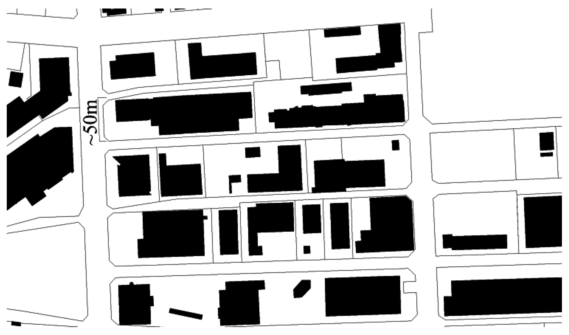
The first test simulations were run in Nekala with a first, preliminary version of the model controlled by stable parameters in the code defining the relative shares of activities on the sites. These values varied according to the number of uses on the site and the site’s current mode of transformation. The resulting pattern formation process was relatively dynamic, but it was difficult to observe how changes in the code affected these patterns.
For the Vaasa case a user interface, preference matrix (Table 7) was introduced. Here it was hypothesized that it could be possible to regulate (and “plan”) on the level of the actors’ interactions, and leaving the global level largely intact. Such an approach would presumably encourage the existing self-organizing mechanism—small scale clustering. Consequently, weight values on each matrix row—for example U1 (housing)—were applied to each activity pair—for example U1 × U1 (housing next to housing). The larger weights and thus more tolerant allocation logics created more heterogeneous spatial configurations. Heavy weights between similar uses increased the degree of agglomeration of this activity. In this experiment the weight values ranged from one to 20, and they were iterated exhaustively by trial and error, simulating various planning decisions. For example, with the matrix the “virtual planner” could experiment with how the high tolerance between housing and all other activities, or low tolerance between housing and industrial uses impacted the model’s dynamics, building overall scenarios or “possible worlds” in a bottom-up manner.
The aim was to explore potential state transitions in the system. Therefore, formal calibration considering the “ruptures” was not possible. The model was calibrated to fit the conditions using visual parameter test echoing Clarke et al. [18]. The weight values were static during the iterations. The time steps were in this case considered hypothetical, since in Vaasa the area’s transformation was not traceable and even manual calibration was not feasible to adjust the computing time steps to reality.
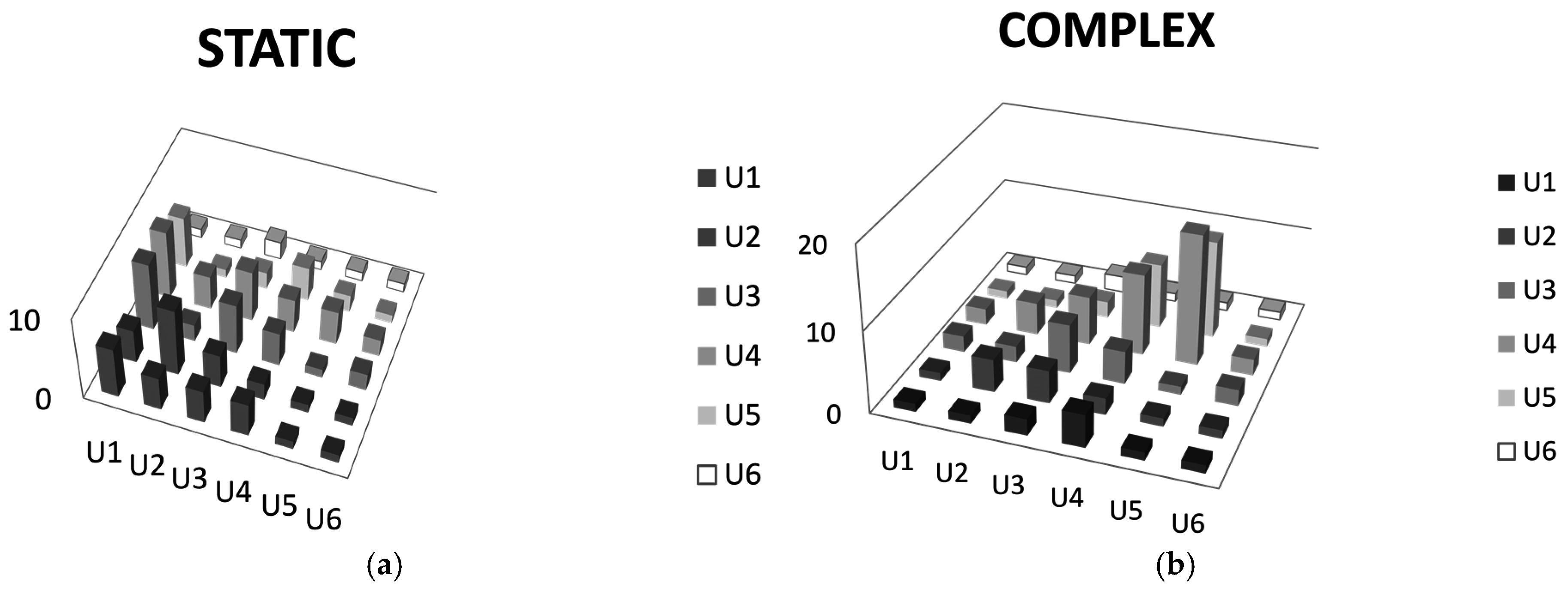
As a result of a negotiation among stakeholders in the planning process, two sets of rules were chosen for simulation. The amount of new housing in the area became a crucial question in the meetings, along with the diversity of other activities, and the first scenario was to support new housing (highest matrix values between housing, U1 × U1). The second one was based on lower weight for housing, implying more mixed uses. However, the static, preserved sites produced a certain diversity in all cases.
The objective was to observe shifts in dynamics resulting from various weight values for each activity pair. The lengths of the runs ranged from 100 to 500 iterations, but extremely long runs (1000 to 2000) were also computed for the potential temporal resilience of the dynamics.

5.1. Performance of the Model

The temporal dynamics and the changes in volumes of activity groups were observed separately for each activity and simulation. The resulting dynamics varied from run to run, depending heavily on the initial matrix values. Different classes of dynamics emerged, and they might occur within a run for different activities simultaneously. For example, the dynamic state of housing might differ from the state of industry with the same initial values. The emerging dynamics were classified into two main categories according the end state, and two sub-categories describing the behavior in more detail (Table 8).

5.1.1. Static States

For the simulations that ended up in a certain end state, two types of static behavior were perceived. In the first case, the system might progress gradually until one use/volume configuration became dominant: The system ended up in a permanent end state. This stagnation might happen simultaneously to one or more activities, and the spatial configuration of sites might vary. In the second case, a dynamic phase in the beginning led to infinite oscillation between only a couple of values on specific sites. The general progress ceased despite these “blinking” (a ”blinker” refers to a well-known case in CA dynamics, oscillation, in the famous Game of Life—see more in [46]) cells; the dynamics can likewise be considered static.
These states were the most common findings. They seemed to correlate with unrestricted, high impact from surrounding housing. In that sense the model appeared to have reflected the urban reality well, as politically the location and surrounding land use caused pressure towards housing development. The static state seemed a plausible, yet not desirable, future for the area.

5.1.2. Dynamic States

As the emphasis was shifted in the matrix from interaction between housing and other uses (U1 × Un(1–6)) towards interaction between office/industrial uses (U4–U5) (see Figure A1 in Appendix A), the behavior of the model changed. First, the volumes started to gradually increase and decrease over time for all activities, resulting in a certain type of coherent yet unpredictable pulse emerging from phases of higher and lower utilization rate on the sites. A certain order seemed to emerge within the system, with measurable cycle length. The changes in the rule set (matrix values) have a marked influence over the dynamics of these periods: With certain rule sets (see the optimum configurations in Table 9) the system gravitated towards a periodic, non-uniform state. The period length was in flux, mostly oscillating between 10 and 12 time steps, revealing dynamics far more diverse than before. Some of these cyclical states started with a stochastic phase, soon settling onto predictable periods (see, e.g., Simulations 207, 212; Supplementary material, Figures S3–S8).
With a very particular set of matrix values (Table 9) the model’s behavior changed radically again. The uses except housing remained periodic, but the lengths of the cycles and degree of predictability seemed to change slightly for different activities. For example, in some cases retail gravitated to a somewhat mixed state with both periodic and more unpredictable phases. The most remarkable shift towards a higher degree of complexity was perceived for housing. Similarly, to the periodic states, the simulation started with a seemingly stochastic phase, soon starting to gravitate towards a certain cycle often with a length of 10, 11 or 12, or occasionally also any random value (Supplemetary material, Figures S3–S8). The period might reoccur from two to as many as 18 times (see e.g., Simulation 190, Figure S9 in Supplementary material). Various cycles might occur during one simulation. Despite these short, constantly emerging and disappearing cycles, the overall dynamics of the system was decidedly unpredictable. This oscillation seemed to continue infinitely even with remarkably long runs (up to 2000 iterations) (see Supplementary material: Complex behavior, Figures S9–S14).
Within many of these simulation runs another new feature emerged, also only with the same complex rule set. While the system balanced between more and less ordered states, a very accurate period of 145 time steps occurred within nearly all runs (see e.g., Simulations 158, 170, 177, 202 in Supplementary material, Figures S11–S14.). Apparently, this period was independent of the state of the system, and was continuous during both the periodic and less predictable states. Perhaps the most interesting feature of this regeneration cycle of 145 time steps was its dynamic stability: in 87% of cases it appeared as the seventeenth cycle, that is, 16 regeneration cycles emerged between two cycles of 145 (for example, the overall volume of the area might have peaked after 27, 12, 10, 34, etc. iterations 16 times before the maxim occurred again after 145 iterations (see Supplementary material, for example Figures S11–S14); then the process resumed, repeatedly). The lengths of the other recurring cycles—for example those of 10 or 12—were all less predictable. The input for the model stayed the same. There is no reference in the literature to this type of CA dynamics where several different nested dynamics co-exist on many levels. This finding may indicate an extremely high level of complexity of the system, but remains to be scrutinized in future studies.

5.2. Validation

These results were visually clearly observable. For validation, I followed the ideas of Langton [8] and Wuenche [13] for entropy measurement of the patterns. The entropy values for the results were calculated for the whole system after simulation. The aim was to discover the differences in overall diversity and predictability.
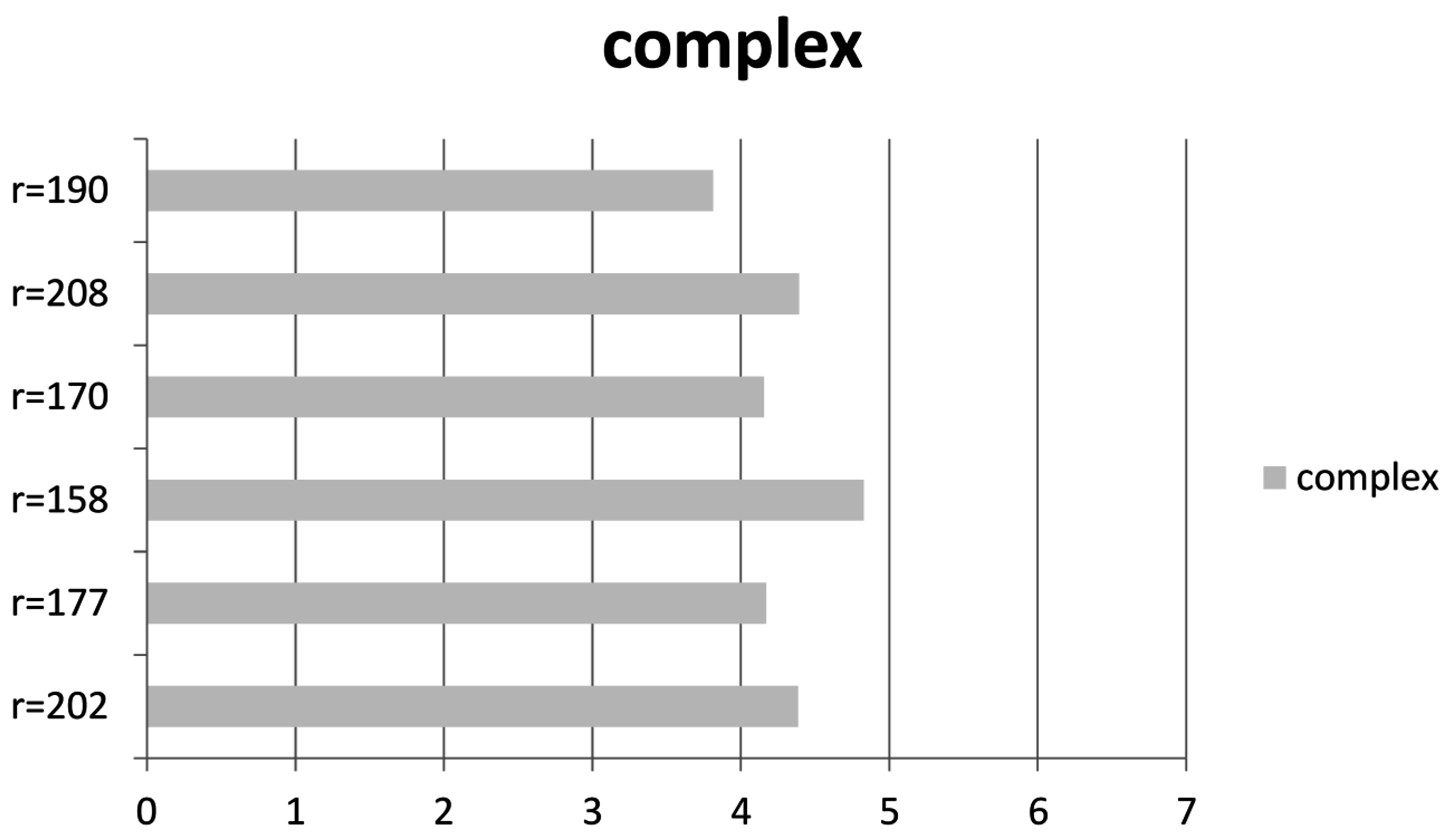
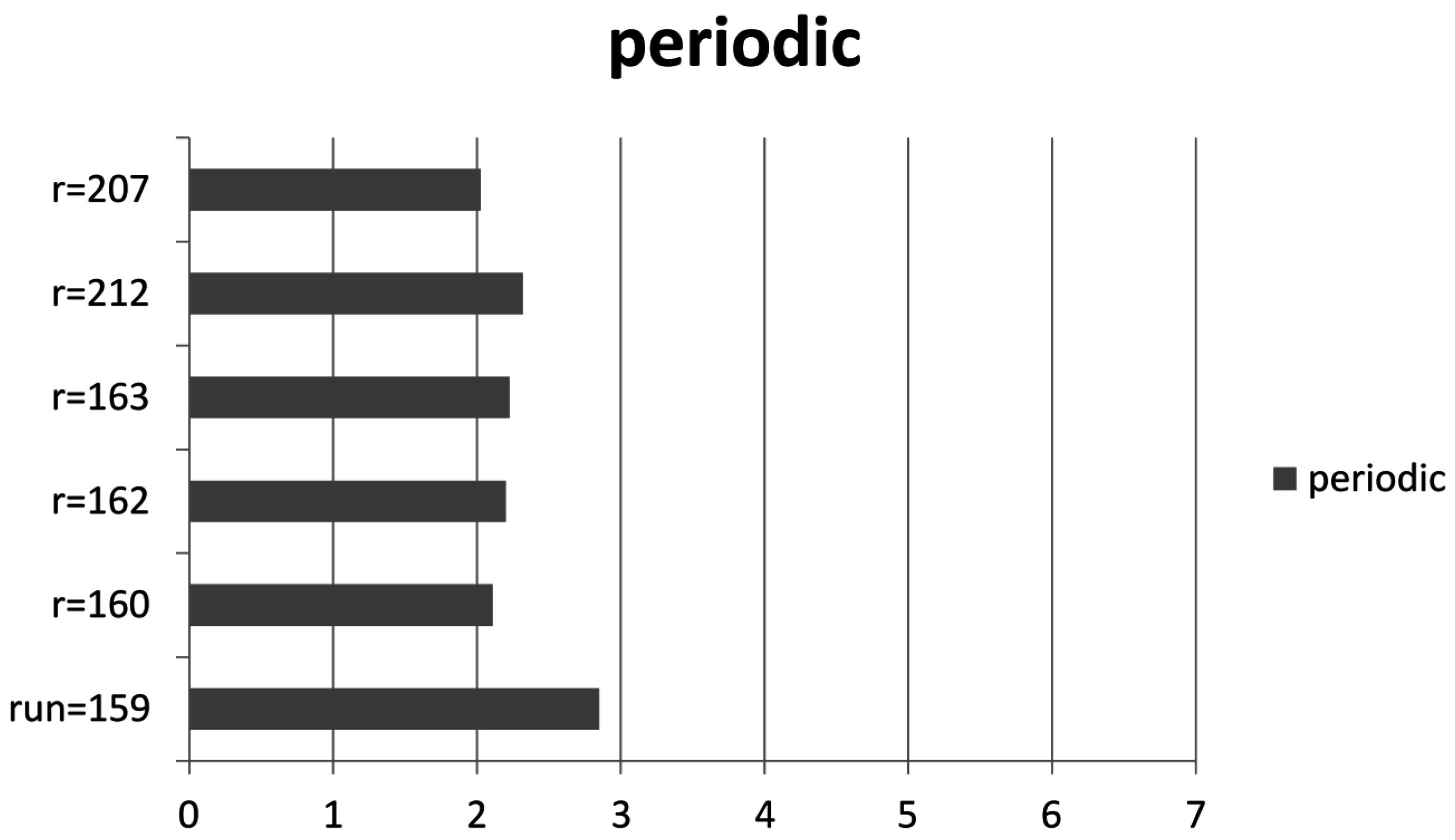
Six examples of periodic and six of complex behavior were chosen at random from the 60 data sets which passed the visual evaluation test. The entropy for the system was calculated according to Equation (2).
j = 1 N s j log 2 s j
where s j is the relative share t / t a l l of the entities; t is the number of a certain regeneration cycle; and tall is the number of different cycles in that run. The resulting entropy values are presented in Table 10. This equation describes the overall entropy of the simulation after the runs are completed, providing an estimated level of complexity in regards of time steps between changes in utilization of building right. (For example, for a periodic run 160, the cycle of 10 occurred 72 times out of a total of 178 different cycles. Hence, for run 160, s j = 72:178 = 0.040449 and consequently, log 2 s j = −1.3058. Thus s j log 2 s j = 0.5282. This calculation was carried out for each cycle (10, 11, 12, 16, 22, etc.) for the total sum, yielding the entropy value of run 160).
The results indicate a clear dispersion between highly ordered, periodic, and more unpredictable, complex states. All the entropy values for periodic states were below 2.86, while for complex states they ranged from 3.80 and 4.90 (Table 8, Figure 6 and Figure 7) (for the graphical representation of the dynamics of these systems, see Supplementary material, Figures S3–S14).
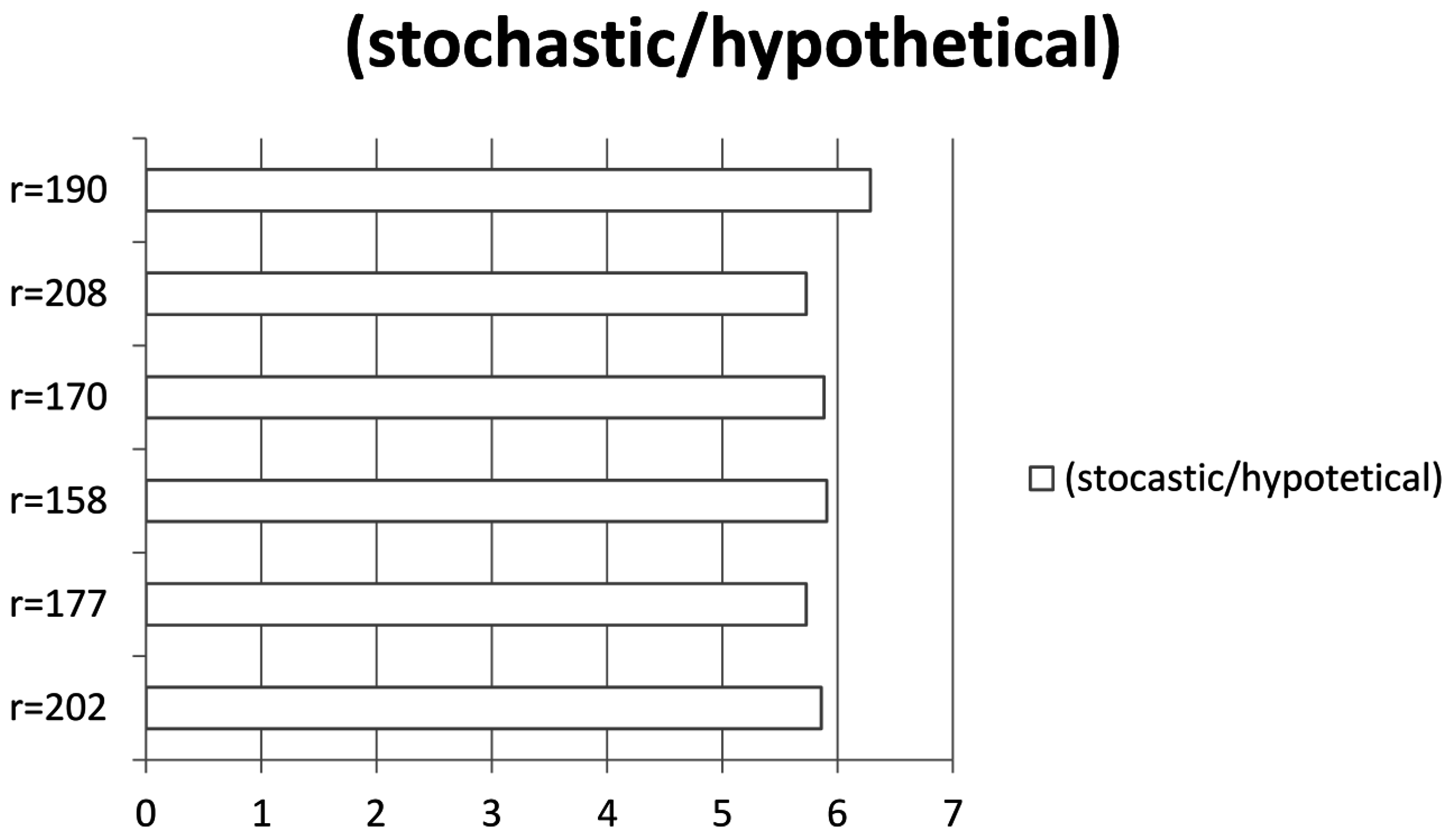
Since no chaotic state was perceived in this study, a stochastic set was created for purposes of comparison, indicating the maximum value of entropy in the system. For this set the entropy was calculated in a hypothetical case using the data set resulting in complexity and calculating its entropy assuming all values to be unique, occurring only once. As expected, the degree of entropy for these stochastic comparison groups was high, all of them above 5.70 (Figure 8).
These results indicate that the periodic state is far more ordered than the complex state, but that the observed complexity was not totally stochastic.
The limitation of this static method of measuring entropy is that it only measures the number of cycles in total and not their temporal frequencies or the potential altering of the periodic and unpredictable phases. For example, in Simulation 190 (Supplementary material, Figure S9), a cycle of 11 forms a period, occurring three times successively between time steps 30 and 32, four times between 63 and 66, and four times again between time steps 51 and 57 implying the relatively high order in these phases. Therefore, this feature needed to be evaluated visually, or by exploring complementary indicators beyond the scope of this study. However, although Equation (2) is static, since it measures the occurrence of the time steps (tn+1tn) between changes, it results in a fairly good representation of the overall entropy of the dynamics. The static states were not included since no measurable period occurred.

5.3. Discussion

This paper contemplated a local scale relaxed urban CA model. The research proved that such a two-dimensional, irregular CA with integrated volume and activity types is capable of simulating the main classical dynamic states typically studied using 1-D CA: Various static, periodic and complex states. Furthermore, the validation indicates that, following the core literature, entropy levels of complex states were indeed between the two extremes (for stochastic and static), thus pointing out the most preferable dynamics for urban evolution.
In this study the transition of these systems from one dynamic state to another did not occur abruptly. On the contrary, the process seemed rather continuous and gradual: as the stress in the matrix was shifted from relations between housing, retail, and services (U1–U3 × U1–U3) towards office/industrial uses (U4–U5 × U4–U5) (Appendix A Figure A1), the dynamic states also seemed to shift gradually first from static/oscillating states to periodic states with a stochastic phase at the beginning towards more complex dynamics. Only one set of matrix values produced extremely complex behavior (Table 9) referring to high sensitivity to initial conditions.
The results suggest that in order to support the continuous states in this modeling case, housing needed to be restricted, while office and light industrial uses needed to be encouraged. The impact of housing on dynamics is not surprising given the volume of the surrounding housing area. However, the complex dynamics for housing is undoubtedly caused by non-linear processes and hence could hardly be discovered in a planning process without a microsimulation. Interestingly, rather high values were also required for offices U4 × U4 and industry U5 × U5 for dynamic continuity. No such effect was observed for activities retail and services. It is plausible that the few static sites in the area formed certain kernels (consisting of retail, services, offices and light industry), and supported the emergence of these actors, but it does not explain the high values required for offices and industry. It is possible that such a surprising impact could be explored further using, for example, complex networks, and emphasizing the number of linkages between actors and the general topology of the nets. Since the objective was to use the existing configurations as the initial state for the CA, such complex interconnectedness of these mechanisms was beyond the scope of this study. The results also highlight the fact that complex interactions between scale levels are not linear and may be extremely unpredictable. In this sense the surprising role of offices and light industry was somewhat noticeable, even though in this case their impact on dynamics in reality is not that self-evident.
In addition, the model corresponds with the reality also in that the static states can be considered analogical with a traditional, hierarchical planning process, in which the plan consolidates a certain static position. Implemented in complex cities in a state of flux, this implies a relevant yet burdensome task of constant, incremental updating of plans. Apparently certain level of flexibility is needed.
However, this modeling experiment indicates that total freedom would not be preferable. Even though the total control of the system will most probably lead to stagnation, a certain degree of guidance is necessary for the process to achieve the most desirable outcome, such as high diversity promoting the evolution of the city. In this sense, the results support the intuition: the maneuvers promoting the diversity of activities in the model produced the most dynamic outcomes.
A couple of limitations concerning the relationship between models and reality overall are worthy of note. This model is based on real data and used in a real planning case, and the results appeared intuitively fairly logical. For example, the housing development could indeed become dominant over other uses. However, the model can at its best predict the future only for a short time span since in complex systems, the future is predictable only in a stable state. Hence, applying the complexity framework underlines the intrinsic nature of the world as, first, an evolutionary system with qualitative transitions impossible to predict, and secondly, its chaotic characteristics, especially in the proximity of these transitions. The system might change drastically due to small initial changes, or not react to larger ones and adapt. One relevant option to respond to this dilemma is, as in this paper, to exhaustively study the dynamics emerging from the simulations instead of for example spatial outcomes. Even then, the simulation results might differ from reality, and hence in planning it is necessary to evaluate the implementations constantly in trial-and-error manner.
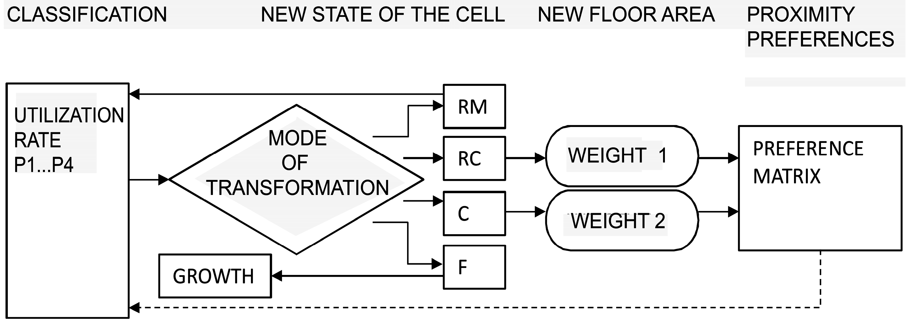
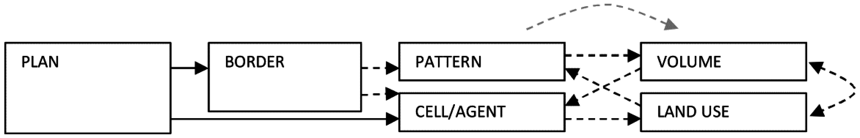
Furthermore, another limitation follows from the configuration of the model. While modeling we stand on the fine line between simplicity and complicatedness. The more detailed the configuration selected for the sake of accuracy, the more difficult it may become to interpret which rules are responsible for a certain model behavior. Hence, several configurational limitations also emerge for the model presented in this paper. For simplicity, the model is based on certain assumptions of agglomeration and regression tendency of activities. In reality, other mechanisms also impact urban dynamics, such as land/property rent, accessibility, synergy between non-similar activities or other externalities. In addition, despite the relaxations, the feedback from the higher level and the outside world was rather limited. In addition, interaction between activities and their environment was contemplated only conceptually to maintain the model simple (Figure 2). For a solution providing greater accuracy and more relevant feedback, possible future studies could therefore include research on other mechanisms of self-organization, studies on the complex linkages and interdependencies between various interacting actors and networks operating on various scales, and comparative studies in other areas.
However, despite the limitations, the model introduced in this paper could be utilized as a good policy-relevant model, which, in Helen Couclelis’ [47] words does not provide instructions for decision-makers on what to do, but instead, on what not to do. In city planning, this would mean, first, acknowledging the uncertainty intrinsic in complexity thinking, but secondly, understanding that urban processes, such as the dynamics that drives location decisions of activities, occur bottom up and their guidance requires setting guidelines rather than of imposing controls.
In such an environment, more flexible planning could provide a frame for urban processes, but the potential impact of the frame must be scrutinized—in this endeavor micro simulations are useful, along with other “complexity planning tools” such as measurement based on fractality, scaling or computation [32,55,56]. In practice, with micro simulation models it is possible to model the environmental factors affecting actors, and then by altering the virtual “planning rules”, for example permitted proximities or other factors, to learn how the guidelines affect the dynamics. Actual decisions could then be based on these findings in a flexible manner, thus supporting self-organization, resilience, city evolution, and continuity of autonomous socio-cultural processes in the city.

Supplementary Materials

The following are available online at www.mdpi.com/1099-4300/19/1/12/s1, Video S1: Complex behavior of the model (housing); Video S2: Periodic behavior of the model (Industrial uses); Video S3: A “blinker” or static/oscillating behavior. Figure S1: Legend for Videos S1 and S3 (housing, volumes); Figure S2: Legend for Video S2 (industrial uses, volumes); Figures S3–S15, Graphical presentation of the model dynamics.

Acknowledgments

The research and data collection were funded by TEKES (the Finnish Funding Agency for Innovation) and Tampere University of Technology Graduate Program. Part of the theoretical work was carried out at the University of Washington, Seattle, USA, funded by the Valle Scholarship, UW Seattle. I would also like to thank Anssi Joutsiniemi for writing the code for the model, and three anonymous reviewers who helped me to develop the article profoundly.

Conflicts of Interest

The author declares no conflict of interest.

Appendix A

Figure A1. Weights for proximity preferences among activity types resulting in different dynamic states: U1, housing; U2, retail; U3, services; U4, offices; U5, light industry; U6, warehouses. (a) Matrix values for static states; (b) Matrix values for the complex states.
Entropy 19 00012 g009

References

  1. Haken, H. Information and Self-Organization: A Macroscopic Approach to Complex Systems; Springer: Berlin/Heidelberg, Germany, 2010. [Google Scholar]
  2. Holland, J.H. Emergence—From Chaos to Order; Perseus Books: Cambridge, MA, USA, 1998. [Google Scholar]
  3. Kauffman, S. The Origins of Order: Self-Organization and Selection in Evolution; Oxford University Press: Oxford, UK, 1993. [Google Scholar]
  4. Kauffman, S. At Home in the Universe: The Search for the Laws of Self-Organization and Complexity; Oxford University Press: Oxford, UK, 1995. [Google Scholar]
  5. Portugali, J. Self-Organization and the City; Springer: Berlin/Heidelberg, Germany; New York, NY, USA, 1999. [Google Scholar]
  6. Walker, B.; Salt, D. Resilience Thinking: Sustaining Ecosystems and People in a Changing World; Island Press: Washington, DC, USA, 2012. [Google Scholar]
  7. Levin, S.A. Ecosystems and the biosphere as complex adaptive systems. Ecosystems 1998, 1, 431–436. [Google Scholar] [CrossRef]
  8. Langton, C.G. Studying Artificial Life with Cellular Automata. Physica D 1990, 22, 120–149. [Google Scholar] [CrossRef]
  9. Kugler, P.N.; Turvey, M.T. Information, Natural Law, and the Self-Assembly of Rhythmic Movement; Routledge: London, UK, 1987; pp. 52–53. [Google Scholar]
  10. Wolfram, S. Universality and Complexity in Cellular Automata. Physica D 1984, 10, 1–35. [Google Scholar] [CrossRef]
  11. Braga, G.; Cattaneo, G.; Flocchini, P.; Quaranta, V.C. Pattern growth in elementary cellular automata. Theor. Comput. Sci. 1995, 145, 1–26. [Google Scholar] [CrossRef]
  12. Culik, K., II; Yu, S. Undecidability of CA classification schemes. Complex Syst. 1988, 2, 177–190. [Google Scholar]
  13. Wuenche, A. Classifying Cellular Automata Automatically; finding gliders, filtering, and relating space-time patterns, attractor basins, and the Z parameter. Complexity 1999, 4, 47–66. [Google Scholar] [CrossRef]
  14. Rienow, A.; Goetzke, R. Supporting SLEUTH-Enhancing a cellular automaton with support vector machines for urban growth modeling. Comput. Environ. Urban Syst. 2015, 49, 66–81. [Google Scholar] [CrossRef]
  15. White, R.; Uljee, I.; Engelen, G. Integrated modelling of population, employment and land-use change with a multiple activity-based variable grid cellular automaton. Int. J. Geogr. Inf. Sci. 2012, 26, 1251–1280. [Google Scholar] [CrossRef]
  16. Batty, M.; Xiu, Y.; Sun, Z. Modelling urban dynamics through GIS-based cellular automata. Comput. Environ. Urban Syst. 1999, 23, 205–233. [Google Scholar] [CrossRef]
  17. Caruso, G.; Peeters, D.; Cavailhès, J.; Rounsevell, M. Spatial configurations in a periurban city. A cellular automata-based microeconomic model. Reg. Sci. Urban Econ. 2007, 37, 542–567. [Google Scholar] [CrossRef]
  18. Clarke, K.C.; Hoppen, S.; Gaydos, L. Methods and techniques for rigorous calibration of a cellular automaton model of urban growth. In Proceedings of the Third International Conference/Workshop on Integrating GIS and Environmental Modeling, Santa Fe, NM, USA, 21–25 January 1996; pp. 21–25.
  19. Li, X.; Yeh, A.G.-O. Modelling sustainable urban development by the integration of constrained cellular automata and GIS. Int. J. Geogr. Inf. Sci. 2000, 14, 131–152. [Google Scholar] [CrossRef]
  20. Portugali, J.; Benenson, I. Artificial planning experience by means of a heuristic cell-space model: Simulating international migration in the urban process. Environ. Plan. A 1995, 27, 1647–1665. [Google Scholar] [CrossRef]
  21. White, R.; Engelen, G. Cellular automata and fractal urban form: A cellular modelling approach to the evolution of urban land use patterns. Environ. Plan. A 1993, 25, 1175–1199. [Google Scholar] [CrossRef]
  22. White, R.; Engelen, G.; Uljee, I. The use of constrained cellular automata for high-resolution modelling of urban land use dynamics. Environ. Plan. B 1997, 24, 323–343. [Google Scholar] [CrossRef]
  23. Schelling, T.C. Dynamic Models of Segregation. J. Math. Soc 1971, 1, 143–186. [Google Scholar] [CrossRef]
  24. Fujita, M. Towards the new economic geography in the brain power society. Reg. Sci. Urban Econ. 2007, 37, 482–490. [Google Scholar] [CrossRef]
  25. Manson, S.; O’Sullivan, D. Complexity theory in the study of space and place. Environ. Plan. A 2006, 38, 677–692. [Google Scholar] [CrossRef]
  26. Porter, M. Clusters and the New Economics of Competition Source. Harv. Bus. Rev. 1998, 76, 77–90. [Google Scholar] [PubMed]
  27. Florida, R. The Rise of the Creative Class and How It’s Transforming Work Leisure, Community and Everyday Life; Basic Books: New York, NY, USA, 2000. [Google Scholar]
  28. Hautamäki, A. Luova Talous ja Kulttuuri Innovaatiopolitiikan Ytimessä; Publications of the Finnish Ministry of Education and Culture: Helsinki, Finland, 2009.
  29. Allen, P. Cities and Regions as Self-Organizing Systems; Taylor & Francis: Oxford, UK, 2004. [Google Scholar]
  30. Shane, D.G. Recombinant Urbanism—Conceptual Modeling in Architecture, Urban Design and City Theory; John Wiley & Sons Ltd.: London, UK, 2005. [Google Scholar]
  31. Oswald, F.; Baccini, P. Netzstadt—Designing the Urban; Birkhäuser: Basel, Switzerland; Boston, MA, USA; Berlin, Germany, 2003. [Google Scholar]
  32. Partanen, J. Indicators for self-organization potential in urban context. Environ. Plan. B 2015, 42, 951–971. [Google Scholar] [CrossRef]
  33. DeLanda, M. Philosophy and Simulation: The Emergence of Synthetic Reason; Bloomsbury Publishing: New York, NY, USA, 2011. [Google Scholar]
  34. Stevens, D.; Dragićević, S. A GIS-based irregular cellular automata model of land-use change. Environ. Plan. B 2007, 34, 708–724. [Google Scholar] [CrossRef]
  35. Reed, M.; Harvey, D.L. The new science and the old: Complexity and realism in the social sciences. J. Theory Soc. Behav. 1992, 22, 353–380. [Google Scholar] [CrossRef]
  36. Batty, M.; Longley, P.A. Fractal Cities: A Geometry of Form and Function; Academic Press: New York, NY, USA, 1994. [Google Scholar]
  37. Hillier, B. Space Is the Machine. A Configurational Theory of Architecture. 2007. Available online: http://discovery.ucl.ac.uk/3881/1/SITM.pdf (accessed on 3 June 2014).
  38. Malmberg, A.; Maskell, P. The elusive concept of localization economies: Towards a knowledge-based theory of spatial clustering. Environ. Plan. A 2002, 34, 429–449. [Google Scholar] [CrossRef]
  39. O’Sullivan, A. Urban Economics; McGraw-Hill Irwin: New York, NY, USA, 2009. [Google Scholar]
  40. Marshall, A. Principles of Political Economy; Maxmillan: New York, NY, USA, 1890. [Google Scholar]
  41. Crutchfield, J.P.; Young, K. Computation at the onset of chaos. In The Santa Fe Institute; Westview: Boulder, CO, USA, 1988. [Google Scholar]
  42. Kurka, P. Languages, equicontinuity and attractors in cellular automata. Ergod. Theory Dyn. Syst. 1997, 17, 417–433. [Google Scholar] [CrossRef]
  43. Gutowitz, H.A. A hierarchical classification of cellular automata. Physica D 1990, 45, 136–156. [Google Scholar] [CrossRef]
  44. Gilman, R.H. Classes of linear automata. Ergod. Theory Dyn. Syst. 1987, 7, 105–118. [Google Scholar] [CrossRef]
  45. Sunter, K. Classifying circular cellular automata. Physica D 1990, 45, 386–395. [Google Scholar]
  46. Gardner, M. The fantastic combinations of John Conway’s new solitaire game ‘Life’. Sci. Am. 1970, 223, 120–123. [Google Scholar] [CrossRef]
  47. Couclelis, H. Modeling frameworks, paradigms, and approaches. In Geographic Information Systems and Environmental Modeling; Clarke, K.C., Parks, B.E., Crane, M.P., Eds.; Longman & Co.: New York, NY, USA, 2000; pp. 1–15. [Google Scholar]
  48. Santé, I.; García, A.M.; Miranda, D.; Crecente, R. Cellular automata models for the simulation of real-world urban processes: A review and analysis. Landsc. Urban Plan. 2010, 96, 108–122. [Google Scholar] [CrossRef]
  49. Shi, W.Z.; Pang, M.Y.C. Development of Voronoi-based cellular automaton integrated dynamic model for geographical information systems. Int. J. Geogr. Inf. Sci. 2000, 14, 455–474. [Google Scholar] [CrossRef]
  50. O’Sullivan, D. Exploring spatial process dynamics using irregular cellular automaton models. Geogr. Anal. 2001, 33, 1–18. [Google Scholar] [CrossRef]
  51. Couclelis, H. Cellular worlds: A framework for modeling micro-macro dynamics. Environ. Plan. A 1985, 17, 585–596. [Google Scholar] [CrossRef]
  52. O’Sullivan, D.; Torrens, P.M. Cellular models of urban systems. In Theory and Practical Issues on Cellular; Bandini, S., Worsch, T., Eds.; Springer: London, UK, 2001; pp. 108–116. [Google Scholar]
  53. Agarwal, C.; Green, G.M.; Grove, J.M.; Evans, T.P.; Schweik, C.M. A Review and Assessment of Land-Use Change Models: Dynamics of Space, Time, and Human Choice. 2002. Available online: https://www.nrs.fs.fed.us/pubs/gtr/gtr_ne297.pdf (accessed on 28 December 2016).
  54. DiPasquale, D.; Wheaton, W. Urban Economics and Real Estate Markets; Prentice Hall: Upper Saddle River, NJ, USA, 1996. [Google Scholar]
  55. De Roo, G.; Hillier, J.; van Wezemael, J. (Eds.) Complexity and Planning: Systems, Assemblages and Simulations. New Directions in Planning Theory; Ashgate: Farnham, UK, 2012.
  56. Batty, M.; Marshall, S. Centenary paper: The evolution of cities: Geddes, Abercrombie and the new physicalism. Town Plan. Rev. 2009, 80, 551–574. [Google Scholar] [CrossRef]
Figure 1. Conceptual model. Interactions between variables; temporal (broken lines), stable (solid lines). Feedback from pattern to actors is implied in decay of overcrowded clusters—typically of CA, the model does not observe explicitly the global level patterns.
Entropy 19 00012 g001
Figure 2. Degree of interaction between activities and their environment for classification of activities: U1, housing; U2, retail; U3, services; U4, offices; U5, light industry; and U6, warehouses. Local Access refers to the local interaction between the site and its environment—how easy it is to access the site, for example, from the street. Interference refers to the level of “disturbance” it tolerates—for example, regarding noise or air quality; and Flow to moving of goods and people to/from the site, implying global accessibility by car, truck etc. The classifications were made on the basis of these assumed relationships. (For example, the requirements for housing regarding disturbance (environmental “interference”) due to noise, smells or heavy traffic differ from those for retail or warehouses. Similarly, some activities need easy access from the street with less privacy, while others benefit from being part of the higher-scale networks, providing constant flows of customers, goods, or material).
Entropy 19 00012 g002
Figure 3. Legal site division and existing buildings. Source: City of Tampere, Finland.
Entropy 19 00012 g003
Figure 4. Modes of cell transformation according to their utilization rates. P-1: “empty”, FAR = 0–0.1; P-2: “nearly-empty”, FAR = 0.1–0.3; P-3: “nearly-full”, FAR = 0.3–0.7; P-4: “full”, FAR = 0.7–1. For example, an almost empty cell is likely to be filled more, but also to be reconstructed—at presumably fairly low demolition costs of smaller buildings, whereas nearly full sites might be considered the most resistant to physical changes, but the new additions or uses may occupy these sites easily (see also Table 6).
Entropy 19 00012 g004
Figure 5. Operational chart of the model.
Entropy 19 00012 g005
Figure 6. Entropy values (i) for six data sets visually classified as “complex”; 3.8 > i > 4.9.
Entropy 19 00012 g006
Figure 7. Entropy values (i) for six data sets visually classified as “periodic”; 2.0 > i > 2.85.
Entropy 19 00012 g007
Figure 8. Entropy values (i) for six hypothetical classes with maximal stochasticity; i > 5.5.
Entropy 19 00012 g008
Table 1. Wolfram’s [10] classification of evolution of dynamic cellular states.
1Homogeneous state
2Simple stable or cyclical/periodic structures
3Chaotic pattern
4Complex localized structures
Table 2. Classification of the evolution of dynamic cellular states by Braga et al. [11].
1Patterns disappear after a finite transient
2All patterns stay limited under iteration of the global transition function
3At least one pattern grows indefinitely
Table 3. Analogies between cellular states and dynamic systems. The periodic and cyclical are used in this paper interchangeably.
CA DynamicsDynamic Systems Analogue
A spatially homogeneous stateLimit points
A sequence of simple stable/periodic structuresLimit cycles
Chaotic behaviorChaotic (strange) attractors
Complicated localized structuresUnspecified
Table 4. Wuenche’s classification of evolution of dynamic cellular states. Entropy level increases from ordered to complex and chaotic states—complex having intermediate state of entropy.
1OrderedLow degree of entropy in system
2ComplexIntermediate degree of entropy in system
3ChaoticHigh degree of entropy in system
Table 5. Relations and directions of interaction between variables (see also Figure 1). In this study, the plan is considered static and unresponsive (the “PLAN” column is empty), unlike in some cases in the reality.
EntitySite (Cell)PatternUseVolumeBorderPlan
Site bottom uptop downtop down
Pattern feedbackfeedback
Use bottom upinteractioninteraction
Volume bottom upinteractioninteraction
Border top downtop down
Plantop down top downtop downtop down
Table 6. Transformation rule 2: The type of transformation depends on the state of the site.
State of the SiteMost Probable ProcedureThe Motive
vacantbuild a new buildingto use the building right
nearly-empty <10%demolish (fill up)to use the building right more effectively: low demolition costs
nearly-fullfill up (change)to use the building right more effectively: demolition costs above the threshold (It is assumed that there is a threshold value defining the shifts from one mode of transformation to another. E.g., a limit when it becomes more profitable to reconstruct the site, taking into account the demolition costs/m3 and new/old FAR. The demolition costs could be calculated, see e.g., DiPasquale and Wheaton [54], p. 85. In this theoretical approach, the classification of the sites is based on estimates.)
fullremain/change/fill/reconstruct, e.g., 0.6/0.3/0.01/0.99 (These values can be changed to fit the circumstances depending on the case at issue.)certain inertia on the full site; however, once the site is full, it will eventually be developed and reconstructed (no more space for additions). tendency to change if one use starts to dominate the neighborhood = high FA
Table 7. Preference matrix which serves as a planner’s user interface: the values increase the likelihood of the two activities being located near to each other. Changing the values makes it possible to learn from their impact on the model dynamics.
U1U2U3U4U5U6
U1 µ 1 µ 2 µ 3 µ 4 µ 5 µ 6
U2 µ 7 µ 8 µ 9 µ 10
U3 µ 11 µ 12 µ 13
U4 µ 14 µ 15
U5 µ 20
U6
µ 1   t o   n = 1…20.
Table 8. Dynamic states of the model. In an oscillating system less complex than periodic state usually two or three values take turns.
Type 1Type 2
staticstagnationoscillation
dynamiccyclical/periodiccomplexity
Table 9. Optimum rule sets resulting in different dynamic states. The values (1 to 20) represent the relative attraction between those activities. For example, in rule set 1, attraction is fairly equal. For rule set 2, office/industry is stressed. In rule set 3, in addition to that, the housing is restricted. (Note that the states with rule set 1 and 2 were remarkably resistant to changing matrix values, for the rule set 3 yielding complex dynamics the configuration was unique—only one configuration of matrix values yielded complex dynamics).
EmphasisMatrix ConfigurationResulting Dynamics
rule set 1. optimum exampleall uses: values range from low to moderate (1–8)644411stagnating/oscillating dynamics; oscillation increased as the U1 × Un(1–6) (attraction between housing and other activities) values decreased
484211
826412
846442
612421
112111
rule set 2. optimum exampleU5 × U5 (small industry) and U4 × U4 (services) are high (µ > 10), other values are moderate (µ 2–8)242411continuous, periodic (cyclical) dynamics (for all activities)
442211
226412
24610162
1128121
112111
rule set 3. unique configurationU1 × U1 (housing) is low (µ = 1), and U4 × U4 (services) and U5 × U5 (small industry) are high (µ > 10), other values: moderate (µ 2–8)112411continuous dynamics: - For housing (U1) complex, - For other uses (U2–U6) periodic (cyclical)
144211
226412
24610162
1128121
112111
Table 10. Degrees of entropy, random samples from complex and periodic/cyclical series, compared to a stochastic set.
periodic/cyclicalR = 159R = 160R = 162R = 163R = 212R = 207
2.851342.111392.201352.228232.320392.02637
complexR = 202R = 177R = 158R = 170R = 208R = 190
4.38644.171424.828934.15564.392623.81511
(stochastic/hypothetical)R = 202R = 177R = 158R = 170R = 208R = 190
5.85795.72795.906895.882645.727926.285

