Foliations-Webs-Hessian Geometry-Information Geometry-Entropy and Cohomology

Abstract

Let us begin by considering two book titles: A provocative title, What Is a Statistical Model? McCullagh (2002) and an alternative title, In a Search for Structure. The Fisher Information. Gromov (2012). It is the richness in open problems and the links with other research domains that make a research topic exciting. Information geometry has both properties. Differential information geometry is the differential geometry of statistical models. The topology of information is the topology of statistical models. This highlights the importance of both questions raised by Peter McCullagh and Misha Gromov. The title of this paper looks like a list of key words. However, the aim is to emphasize the links between those topics. The theory of homology of Koszul-Vinberg algebroids and their modules (KV homology in short) is a useful key for exploring those links. In Part A we overview three constructions of the KV homology. The first construction is based on the pioneering brute formula of the coboundary operator. The second construction is based on the theory of semi-simplicial objects. The third construction is based on the anomaly functions of abstract algebras and their abstract modules. We use the KV homology for investigating links between differential information geometry and differential topology. For instance, “dualistic relation of Amari” and “Riemannian or symplectic Foliations”; “Koszul geometry” and “linearization of webs”; “KV homology” and “complexity of models”. Regarding the complexity of a model, the challenge is to measure how far from being an exponential family is a given model. In Part A we deal with the classical theory of models. Part B is devoted to answering both questions raised by McCullagh and B Gromov. A few criticisms and examples are used to support our criticisms and to motivate a new approach. In a given category an outstanding challenge is to find an invariant which encodes the points of a moduli space. In Part B we face four challenges. (1) The introduction of a new theory of statistical models. This re-establishment must answer both questions of McCullagh and Gromov; (2) The search for an characteristic invariant which encodes the points of the moduli space of isomorphism class of models; (3) The introduction of the theory of homological statistical models. This is a pioneering notion. We address its links with Hessian geometry; (4) We emphasize the links between the classical theory of models, the new theory and Vanishing Theorems in the theory of homological statistical models. Subsequently, the differential information geometry has a homological nature. That is another notable feature of our approach. This paper is dedicated to our friend and colleague Alexander Grothendieck.

Contents

• 1 Introduction        4

  • 1.1 The Notation . . . . . . . . . . . . . . . . . . . . . . . . . . . . . . . . . . . . . . . . . . . . 4
  • 1.2 Some Explicit Formulas . . . . . . . . . . . . . . . . . . . . . . . . . . . . . . . . . . . . . 4
  • 1.3 The content of the Paper . . . . . . . . . . . . . . . . . . . . . . . . . . . . . . . . . . . . . 5
• 2 Algebroids, Moduls of Algebroids, Anomaly Functions        8

  • 2.1 The Algebroids and Modules . . . . . . . . . . . . . . . . . . . . . . . . . . . . . . . . . . 8
  • 2.2 Anomaly Functions of Algebroids and of Modules . . . . . . . . . . . . . . . . . . . . . . 9
• 3 The Theory of Cohomology of KV Algebroids and Their Modules        11

  • 3.1 The Theory of KV Cohomology—Version the Brute Formula of the Coboundary Operator 11

    • 3.1.1 The Cochain Complex C_KV. . . . . . . . . . . . . . . . . . . . . . . . . . . . . . . . 11
    • 3.1.2 The Total Cochain Complex C_τ. . . . . . . . . . . . . . . . . . . . . . . . . . . . . . 13
  • 3.2 The Theory of KV Cohomology—Version: the Semi-Simplicial Objects . . . . . . . . . . 14

    • 3.2.1 Extension . . . . . . . . . . . . . . . . . . . . . . . . . . . . . . . . . . . . . . . . . 14
    • 3.2.2 Construction . . . . . . . . . . . . . . . . . . . . . . . . . . . . . . . . . . . . . . . 14
    • 3.2.3 Notation-Definitions . . . . . . . . . . . . . . . . . . . . . . . . . . . . . . . . . . . 15
    • 3.2.4 The KV Chain Complex . . . . . . . . . . . . . . . . . . . . . . . . . . . . . . . . . 16
    • 3.2.5 The V-Valued KV Homology . . . . . . . . . . . . . . . . . . . . . . . . . . . . . . 16
    • 3.2.6 Two Cochain Complexes . . . . . . . . . . . . . . . . . . . . . . . . . . . . . . . . . 17
    • 3.2.7 Residual Cohomology . . . . . . . . . . . . . . . . . . . . . . . . . . . . . . . . . . 18
  • 3.3 The Theory of KV Cohomology—Version the Anomaly Functions . . . . . . . . . . . . . 20

    • 3.3.1 The General Challenge CH$\left(\mathbb{D}\right)$ . . . . . . . . . . . . . . . . . . . . . . . . . . . . . 20
    • 3.3.2 Challenge CH$\left(\mathcal{D}\right)$ for KV Algebras . . . . . . . . . . . . . . . . . . . . . . . . . . . 21
    • 3.3.3 The KV Cohomology . . . . . . . . . . . . . . . . . . . . . . . . . . . . . . . . . . . 23
    • 3.3.4 The Total Cohomology . . . . . . . . . . . . . . . . . . . . . . . . . . . . . . . . . . 24
    • 3.3.5 The Residual Cohomology, Some Exact Sequences, Related Topics, DTO-HEG-IGE-ENT . . . . . . . . . . . . . . . . . . . . . . . . . . . . . . . . . . . 24
• 4 The KV Topology of Locally Flat Manifolds        26

  • 4.1 The Total Cohomology and Riemannian Foliations . . . . . . . . . . . . . . . . . . . . . . 26
  • 4.2 The General Linearization Problem of Webs . . . . . . . . . . . . . . . . . . . . . . . . . . 28
  • 4.3 The Total KV Cohomology and the Differential Topology Continued . . . . . . . . . . . 30
  • 4.4 The KV Cohomology and Differential Topology Continued . . . . . . . . . . . . . . . . . 34

    • 4.4.1 Kernels of 2-Cocycles and Foliations . . . . . . . . . . . . . . . . . . . . . . . . . . 34
• 5 The Information Geometry, Gauge Homomorphisms and the Differential Topology        35

  • 5.1 The Dualistic Relation . . . . . . . . . . . . . . . . . . . . . . . . . . . . . . . . . . . . . . 35

    • 5.1.1 Statistcal Reductions . . . . . . . . . . . . . . . . . . . . . . . . . . . . . . . . . . . 40
    • 5.1.2 A Uselful Complex . . . . . . . . . . . . . . . . . . . . . . . . . . . . . . . . . . . . 40
    • 5.1.3 The Homological Nature of Gauge Homomorphisms . . . . . . . . . . . . . . . . 41
    • 5.1.4 The Homological Nature of the Equation FE^∇∇* . . . . . . . . . . . . . . . . . . . 43
    • 5.1.5 Computational Relations. Riemannian Foliations. Symplectic Foliations: Continued . . . . . . . . . . . . . . . . . . . . . . . . . . . . . . . . . . . . . . . . . 45
    • 5.1.6 RiemannianWebs—SymplecticWebs in Statistical Manifolds . . . . . . . . . . . 49
  • 5.2 The Hessian Information Geometry, Continued . . . . . . . . . . . . . . . . . . . . . . . . 51
  • 5.3 The a-Connetions of Chentsov . . . . . . . . . . . . . . . . . . . . . . . . . . . . . . . . . 53
  • 5.4 The Exponential Models and the Hyperbolicity . . . . . . . . . . . . . . . . . . . . . . . . 55
• 6 The Similarity Structure and the Hyperbolicity        58
• 7 Some Highlighting Conclusions        59

  • 7.1 The Total KV Cohomology and the Differential Topology . . . . . . . . . . . . . . . . . . 59
  • 7.2 The KV Cohomology and the Geometry of Koszul . . . . . . . . . . . . . . . . . . . . . . 60
  • 7.3 The KV Cohomology and the Information Geometry . . . . . . . . . . . . . . . . . . . . 60
  • 7.4 The Differential Topology and the Information Geometry . . . . . . . . . . . . . . . . . . 60
  • 7.5 The KV Cohomology and the Linearization Problem for Webs . . . . . . . . . . . . . . . 60
• 8 B. The Theory of StatisticaL Models        61

  • 8.1 The Preliminaries . . . . . . . . . . . . . . . . . . . . . . . . . . . . . . . . . . . . . . . . . 65
  • 8.2 The Category $\mathcal{FB}(\mathsf{\Gamma },\mathsf{\Xi })$ . . . . . . . . . . . . . . . . . . . . . . . . . . . . . . . . . . . . . . 66

    • 8.2.1 The Objects of $\mathcal{FB}(\mathsf{\Gamma },\mathsf{\Xi })$ . . . . . . . . . . . . . . . . . . . . . . . . . . . . . . . . . 66
    • 8.2.2 The Morphisms of $\mathcal{FB}(\mathsf{\Gamma },\mathsf{\Xi })$ . . . . . . . . . . . . . . . . . . . . . . . . . . . . . . 68
  • 8.3 The Category $\mathcal{GM}(\mathsf{\Xi },\mathsf{\Omega })$ . . . . . . . . . . . . . . . . . . . . . . . . . . . . . . . . . . . . . 68

    • 8.3.1 The Objects of $\mathcal{GM}(\mathsf{\Xi },\mathsf{\Omega })$ . . . . . . . . . . . . . . . . . . . . . . . . . . . . . . . . 68
    • 8.3.2 The Global Probability Density of a Statistical Model . . . . . . . . . . . . . . . . 70
    • 8.3.3 The Morphisms of $\mathcal{GM}(\mathsf{\Xi },\mathsf{\Omega })$ . . . . . . . . . . . . . . . . . . . . . . . . . . . . . . 71
    • 8.3.4 Two Alternative Definitions . . . . . . . . . . . . . . . . . . . . . . . . . . . . . . . 72
    • 8.3.5 Fisher Information in $\mathcal{GM}(\mathsf{\Xi },\mathsf{\Omega })$ . . . . . . . . . . . . . . . . . . . . . . . . . . . . 73
  • 8.4 Exponential Models . . . . . . . . . . . . . . . . . . . . . . . . . . . . . . . . . . . . . . . . 73

    • 8.4.1 The Entropy Flow . . . . . . . . . . . . . . . . . . . . . . . . . . . . . . . . . . . . 74
    • 8.4.2 The Fisher Information as the Hessian of the Local Entropy Flow . . . . . . . . . 75
    • 8.4.3 The Amari-Chentsov Connections in $\mathcal{GM}(\mathsf{\Xi },\mathsf{\Omega })$ . . . . . . . . . . . . . . . . . . . 75
    • 8.4.4 The Homological Nature of the Probability Density . . . . . . . . . . . . . . . . . 76
    • 8.4.5 Another Homological Nature of Entropy . . . . . . . . . . . . . . . . . . . . . . . 77
• 9 The Moduli Space of the Statistical Models        78
• 10 The Homological Statistical Models        83

  • 10.1 The Cohomology Mapping of HSM$(\mathsf{\Xi },\mathsf{\Omega })$ . . . . . . . . . . . . . . . . . . . . . . . . . . . 84
  • 10.2 An Interpretation of the Equivariant Class [Q] . . . . . . . . . . . . . . . . . . . . . . . . 85
  • 10.3 Local Vanishing Theorems in the Category $\mathcal{HSM}(\mathsf{\Xi },\mathsf{\Omega })$ . . . . . . . . . . . . . . . . . . 85
• 11 The Homological Statistical Models and the Geometry of Koszul        88
• 12 Examples        88
• 13 Highlighting Conclusions        91

  • 13.1 Criticisms . . . . . . . . . . . . . . . . . . . . . . . . . . . . . . . . . . . . . . . . . . . . . 91
  • 13.2 Complexity . . . . . . . . . . . . . . . . . . . . . . . . . . . . . . . . . . . . . . . . . . . . . 91
  • 13.3 KV Homology and Localization . . . . . . . . . . . . . . . . . . . . . . . . . . . . . . . . . 91
  • 13.4 The Homological Nature of the Information Geometry . . . . . . . . . . . . . . . . . . . 91
  • 13.5 Homological Models and Hessian Geometry . . . . . . . . . . . . . . . . . . . . . . . . . 92
• A Appendix A        92

  • A.1 The Affinely Flat Geometry . . . . . . . . . . . . . . . . . . . . . . . . . . . . . . . . . . . 93
  • A.2 The Hessian Geometry . . . . . . . . . . . . . . . . . . . . . . . . . . . . . . . . . . . . . . 93
  • A.3 The Geometry of Koszul . . . . . . . . . . . . . . . . . . . . . . . . . . . . . . . . . . . . . 93
  • A.4 The Information Geometry . . . . . . . . . . . . . . . . . . . . . . . . . . . . . . . . . . . . 94
  • A.5 The Differential Topology of a Riemannian Manifold . . . . . . . . . . . . . . . . . . . . 94

1. Introduction

1.1. The Notation

Throughout the paper we use tha following notation. N is the set of non negative integers, Z is the ring of integers, R is the field of real numbers, $C^{\infty }(M)$ is the associative commutative algebra of real valued smooth functions in a smooth manifold M. Let ∇ be a Koszul connection in a manifold M, $R^{\nabla }$ is the curvature tensor of ∇. It is defined by

$$R^{\nabla }(X,Y)={\nabla }_X{\nabla }_Y-{\nabla }_Y{\nabla }_X-{\nabla }_{[X,Y]}.$$

$T^{\nabla }$ is the torsion tensor of ∇. It is defined by

$$T^{\nabla }(X,Y)={\nabla }_{X}Y-{\nabla }_{Y}X-[X,Y].$$

Let X be a smooth vector field in M. $L_X\nabla$ is the Lie derivative of ∇ in the direction $X·\iota (X)R^{\nabla }$ is the inner product by X. To a pair of Koszul connections $(\nabla ,{\nabla }^{*})$ we assign three differential operators. They are denoted by $D^{\nabla {\nabla }^{*}}$, $D^{\nabla }$ and $D_{\nabla }$.

(A.1)

$D^{\nabla {\nabla }^{*}}$ is a first order differential operator. It is defined in the vector bundle $Hom(TM,TM)$. Its values belong to the vector bundle $Hom(T{M}^{\otimes 2},TM)$.

(A.2)

$D^{\nabla }$ and $D_{\nabla }$ are 2nd order differential operators. They are defined in the vector bundle $TM$. Their values belong to the vector bundle $Hom(T{M}^{\otimes 2},TM)$. Let X be a section of $TM$ and let ψ be a section of $T^{*}M\otimes TM$. The differential operators just mentioned are defined by

$$\begin{array}{}\mathrm{(1a)}& \hfill D^{\nabla {\nabla }^{*}}(\psi )={\nabla }^{*}\circ \psi -\psi \circ \nabla ,\mathrm{(1b)}& \hfill D^{\nabla }(X)=L_X\nabla -\iota (X)R^{\nabla },\mathrm{(1c)}& \hfill D_{\nabla }(X)={\nabla }^2(X).\end{array}$$

Part A of this paper is partially devoted to the global analysis of the differential equation

$$FE(\nabla {\nabla }^{*}):D^{\nabla {\nabla }^{*}}(\psi )=O.$$

The solutions to $FE(\nabla {\nabla }^{*})$ are useful for addressing the links between the KV homology, the differential topology and the information geometry.

The purpose of a forthcoming paper is the study of the differential equations

$$F{E}^{*}(\nabla ):D^{\nabla }(X)=0,$$

$$F{E}^{**}(\nabla ):D_{\nabla }(X)=0.$$

In the Appendix A to this paper we overview the role played by the solutions to $F{E}^{**}(\nabla )$ in some still open problems.

1.2. Some Explicit Formulas

Let $x=(x_1,...,x_m)$ be a system of local coordinate functions of M. In those coordinates the Christoffel symbols of both ∇ and ${\nabla }^{*}$ are denoted by ${\mathsf{\Gamma }}_{ij:k}$ and ${\mathsf{\Gamma }}_{ij:k}^{*}$ respectively. We use those coordinate functions for presenting an element $\psi \in \mathcal{M}(\nabla {\nabla }^{*})$ as a matrix $[{\psi }_{ij}]$. Thus by setting $\partial i=\frac{\partial }{\partial x_i}$ one has

$${\nabla }_{\partial i}\partial j={\mathsf{\Gamma }}_{ij:k}\partial k.$$

We focus on $FE(\nabla {\nabla }^{*})$ and of $F{E}^{**}(\nabla )$. They are equivalent to the following system of partial differential equations

$$[S_{ij:k}]:\frac{\partial {\psi }_{kj}}{\partial x_i}-\sum _{1\le \ell \le m}({\mathsf{\Gamma }}_{ij:\ell }{\psi }_{k\ell }-{\mathsf{\Gamma }}_{i\ell :k}^{*}{\psi }_{\ell }j)=0,$$

$$[{\mathsf{\Theta }}_{ij}^k(X)]:\frac{{\partial }^2{X}^k}{\partial x_i\partial x_j}+\sum _{\alpha }[{\mathsf{\Gamma }}_{i\alpha }^k\frac{\partial X^{\alpha }}{\partial x_j}+{\mathsf{\Gamma }}_{j\alpha }^k\frac{\partial X^{\alpha }}{\partial x_i}-{\mathsf{\Gamma }}_{ij\frac{\partial X^k}{\partial x_{\alpha }}}^{\alpha }]+\sum _{\alpha }[\frac{\partial {\mathsf{\Gamma }}_{j\alpha }^k}{\partial x_i}+\sum _{\beta }[{\mathsf{\Gamma }}_{j\alpha }^{\beta }{\mathsf{\Gamma }}_{i\beta }^k-{\mathsf{\Gamma }}_{ij}^{\beta }{\mathsf{\Gamma }}_{\beta }^k\alpha ]]X^{\alpha }=0.$$

In Part A we address the links between the following topics DTO, HGE, IGE and ENT. Those topics are presented as vertices of a square whose centre is denoted by $KVH$.

(1)

DTO stands for Differential TOpology. In DTO, FWE stands for Foliations and WEbs.

(2)

HGE stands for Hessian GEometry. Its sources are the geometry of bounded domains, the topology of bounded domains, the analysis in bounded domains. Among the notable references are [1,2,3]. Hessian geometry has significant impacts on thermodynamics, see [4,5], About the impacts on other related topics the readers are referred to [6,7,8,9,10,11,12].

(3)

IGE stands for Information GEometry. That is the geometry of statistical models. More generally its concern is the differential geometry of statistical manifolds. The range of the information geometry is large [13]. Currently, the interest in information geometry is increasing. This comes from the links with many major research domains [14,15,16]. We address some significant aspects of those links. Non-specialist readers are referred to some fundamental references such as [17,18]. See also [4,19,20,21,22,23]. The information geometry also provides a unifying approach to many problems in differential geometry, see [21,24,25]. The information geometry has a large scope of applications, e.g., physics, chemistry, biology and finance.

(4)

ENT stands for ENTropy. The notion of entropy appears in many mathematical topics, in Physics, in thermodynamics and in mechanics. Recent interest in the entropy function arises from its topological nature [14]. In Part B we introduce the entropy flow of a pair of vector fields. The Fisher information is then defined as the Hessian of the entropy flow.

(5)

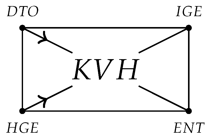
KVH stands for KV Homology. The theory of KV homology was developed in [9]. The motivation was the conjecture of M. Gerstenhaber in the category of locally flat manifolds. In this paper we emphasize other notable roles played by the theory of KV homology. It is also useful for discussing a problem raised by John Milnor in [26].

The conjecture of Gerstenhaber is the following claim.

Every restricted theory of deformation generates its proper cohomology theory [27].

Loosely speaking, in a restricted theory of deformation one has the notion of both infinitesimal deformation and trivial deformation. The challenge is the search for a cochain complex admitting infinitesimal deformations as cocycles. In the present paper, $KVH$ is useful for emphasizing the links between the vertices $DTO$, $HGE$, $IGE$ and $ENT$. That is our reason for devoting a section to $KVH$.

Warning. 

We propose to overview the structure of this paper. The readers are advised to read this paper as through it were a wander around the vertices of the square “DTO-HGE-IGE-ENT”. Thus, depending on his interests and his concerns a reader could walk several times across the same vertex. For instance the information geometry appears in many sections, depending on the purpose and on the aims.

1.3. The content of the Paper

This paper is divided into Part A and Part B.

Part A: Section 1, Section 2, Section 3, Section 4, Section 5, Section 6 and Section 7.

Section 1 is the Introduction. Section 2 is devoted to algebroids, modules of algebroids and the theory of KV homology of the Koszul-Vinberg algebroids. To introduce the KV cohomology we have adopted three approaches. Each approach is based on its specific machinery. However, the readers will face three cochain complexes which are pairwise quasi isomorphic. The KV cohomology is present throughout this paper. At the end of Part B the reader will see that the theory of statistical models is but a vanishing theorem in the theory of KV hohomology. The first approach is based on the pioneering fundamental brute formula of the coboundary operator. Historically, the brute formula is the first to have been constructed [9].

This first approach is used in many sections of this paper. Regarding the theory of deformation of the Koszul Geometry, the KV cohomology is the solution to the conjecture of Gerstenhaber. In the theory of modules of KV algebroids the role played by the KV cohomology is practically SIMILAR to the role played by the Hocshild cohomology in the category of associative alggebroids and their modules. This last remark holds for the role played by the Chevalley-Eilenberg cohomology in the category of Lie algebroids and their modules. Nevertheless, our comparison fails in the theory of Extension of modules over algebroids. In both categories of extensions of modules over associative algebroids and Lie algebroids the moduli space of equivalence class is encoded by cohomology classes of degree one. In the category of extensions of KV modules the moduli space is encoded by a spectral sequence. That was a unexpected feature in [9]. The pioneering coboundary operator of Nijenhuis [28] may be derived from the total brute coboundary operator introduced in [29].

The second approach is based on the notion of simplecial objects.

The third approach is based on the theory of anomaly functions for abstract algebras and their abstract modules. The idea has emerged from recent correspondences with one of my former teachers. The KV anomaly function of a Koszul connection ∇ may be expressed in terms of the ∇-Hessian operators ${\nabla }^2$, namely

$$K{V}_{\nabla }(X,Y,Z)=<{\nabla }^2(Z),(X,Y)>-<{\nabla }^2(Z),(Y,X)>.$$

This approach is a powerful for addressing the relationships between the global analysis, the differential topology and the information geometry. The approach by the anomaly functions suggests many conjectures. Among those conjectures is the following.

Conjecture. Every anomaly function of algebras and of modules yields a theory of cohomology of algebras and modules.

Section 3. This section is devoted to the theory of KV (co)homology of Koszul-Vinberg algebroids. We focus on cohomological data which are used in the paper.

Section 4. This section is devoted the KV algebroids which are defined by structures of locally flat manifold. The KV cohomology theory is used for highlighting the impacts on the differential topology of the information geometry and its methods. We make the most of some relationships between the KV cohomology and the global analysis of the differential equation $F{E}^{*}(\nabla {\nabla }^{*})$. We also sketch the global analysis of the differential equation

$$F{E}^{**}(\nabla ).$$

This leads to the function

$$\mathcal{L}\mathcal{C}\ni \nabla \to r^b(\nabla )\in \mathbb{Z}.$$

We explain how to interpret $r^b$ as a distance. (See the Appendix A to this paper ). For instance, the function $r^b$ gives rise to an numerical invariant $r^b(\mathbb{M})$ which measures how far from being an exponential family is a statistical model $\mathbb{M}$. This result is a significant contribution to the information geometry, see [18,22,24].

Section 5. We are interested in how interact the information geometry, the KV cohomology and the geometry and Koszul. In particular we relate the notion of hyperbolicity and vanishing theorems in the KV cohomology.

Section 6. This section is devoted to the homological version of the geometry of Koszul. Our approach involves the dualistic relation of Amari. The KV cohomology links the dualistic relation with the geometry of Koszul.

Section 7. In this section summarize the highlighting features of Part A.

Part B: Section 8, Section 9, Section 10, Section 11, Section 12, Section 13 and Section 14.

Section 8. This is the starting section of the second part B. This Part B is devoted to new insights in the theory of statistical models. On 2002 Peter McCullar raised the provocative question.

What Is a Statistical Model

Across the world (Australia, Canada, Europe, US) the $McCullag{h}^s$ paper became the object of many criticisms and questions by eminent theoretical and applied statisticians [30].

Part B is aimed at supplying some deficiencies in the current theory of statistical models. We address some criticisms which support the need of re-establishing the theory of statistical model for measurable sets. Those criticisms are used for highlight the lack of both Structure and Relations. Those criticisms also highlight the search of M. Gromov [15]. The need for structures and relations was the intuition of Peter McCullagh. Loosely speaking there is a lack of Intrinsic Geometry in the sense of Erlangen. Subsequently the lack of intrinsic geometry yields other things that are lacking. The problem of the moduli space of models is not studied, although this would be crucial for applied information geometry, and for applied statistics. That might be a key in reading some the controversy about [30].

Section 9. In this section we address the problem of moduli space of statistical models. The problem of moduli space in a category is a major question in Mathematic. It is generally a difficult problem that involves finding a characteristic invariant which encodes the point of the moduli space. Such an invariant is a crucial step toward the geometry and the topology of a moduli space. Among other needs, the problem of encoding the moduli space of models has motivated our need of a new approach, that is to say the need of a theory having nice mathematical structure and relations. In this Part B the problem of the moduli space is solved. To summarize the theorem describing the moduli spaces of statistical models we need the following notation.

A gauge structure in a manifold M is a pair $(M,\nabla )$ where ∇ is a Koszul connection in M. The category of gauge structures in M is denoted by $\mathcal{L}\mathcal{C}(M)$. We are concerned with the vector bundle $T^{*\otimes 2}M$ of bi-linear forms in the tangent bundle $TM$. The sheaf of sections of $T^{*\otimes 2}M$ is denoted by $\mathcal{B}\mathcal{L}(M)$.

The category of m-dimensional statistical models (to be defined) of a measurable $(\mathsf{\Xi },\mathsf{\Omega })$ is denoted by ${\mathcal{GM}}_m(\mathsf{\Xi },\mathsf{\Omega })$. The category of random functors

$$\mathcal{L}\mathcal{C}(M)\times \mathsf{\Xi }\to \mathcal{B}\mathcal{L}(M)$$

is denoted by $\mathcal{F}(\mathcal{L}\mathcal{C},\mathcal{B}\mathcal{L})(M).$ One of the interesting breakthrough in this Part.B is the following solution to the problem of moduli.

Theorem 1.

There exists a functor

$${\mathcal{GM}}_m(\mathsf{\Xi },\mathsf{\Omega })\ni \mathbb{M}\to q_{\mathbb{M}}\in \mathcal{B}\mathcal{L}(M)$$

(2)

which determines a model $\mathbb{M}$ up to isomorphism.

Let p be the probability density of a model $\mathbb{M}$. The mathematical expectation of $q_{\mathbb{M}}(\nabla )$ is defined by

$$E(q_{\mathbb{M}}(\nabla ))={\int }_{\mathsf{\Xi }}p{q}_{\mathbb{M}}(\nabla ).$$

(3)

The quantity $E(q_{\mathbb{M}})(\nabla )$ does not depend on the Koszul connection ∇. It is called the Fisher information of $\mathbb{M}$.

This theorem emphasizes the Search for structure [16].

Section 10. This section is devoted to introduce the category of homological statistical models. This may be interpreted as a variant of the topology of the information. Another approach is to be found in Baudot-Bennequin [31].

The current theory (as in [17]) is called the classical (or local) theory. This means that a statistical model as in [17,18] is derived from the localization of a homological model. Loosely speaking such a model expresses a local vanishing theorem in the theory of homological statistical models.

Section 11. This section is devoted to discussing the links between the geometry of Koszul and the theory of homological statistical models. Those investigations lead to this notable feature.

The Geometry of Koszul, the homological statistical models and the classical information geometry locally look alike.

Section 12. Through Section 9 the framework is the category of equivariant locally trivial fibration. This assumption is weakened in Section 12. We recall the relationships between the Cech cohomology and the theory of locally trivial fiber bundle. We extend the scope of applications of the methods of the information geometry. Those extensions produce some interesting results. Here is an instance.

Theorem 2.

Let M be an oriented compact real analytic manifold and let $C^{\omega }(M^2)$ be the space of real valued analytic functions in $M^2$. There exists a non trivial map of $C^{\omega }(M^2)$ in the family of (positive) stratified Riemannian foliation in M.

Section 13. This Section 13 is a variant of Section 7.

Section 14 is an appendix we have mentioned. It is devoted to overview a few new significant results. Those results are derived from the global analysis of the differential operators

$$\left\{D^{\nabla },D_{\nabla },\nabla \in \mathcal{L}\mathcal{C}(M)\right\}.$$

The solutions to a few open problems are announced.

2. Algebroids, Moduls of Algebroids, Anomaly Functions

The purpose of this section is to introduce basic notions in the algebraic topology of locally flat manifolds.

2.1. The Algebroids and Modules

Given a smooth fiber bundle

$$B\to M$$

the set of smooth sections of B is denoted by $\mathsf{\Gamma }(B)$.

Definition 1.

An (abstract) real algebra is a real vector space $\mathcal{A}$ endowed with a bilinear map

$$\mathcal{A}\times \mathcal{A}\to \mathcal{A}$$

Definition 2.

An (abstract) real two-sided module of an (abstract) algebra $\mathcal{A}$ is a real vector space W with two bilinear mappings

$$\mathcal{A}\times W\to W,$$

$$W\times \mathcal{A}\to W$$

Warning. 

Here algebra means a multiplication $a·b$ without any rule of calculations. So the product $a·b·c$ is meaningless.

Throughout this paper, the smooth manifolds we deal with are connected and paracompact. In a smooth manifold M all geometrical objects we are interested in are smooth as well.

The vector space of smooth vector fields in a manifold M is denoted by $\mathcal{X}(M).$ It is a left module of the associative commutative algebra $C^{\infty }(M)$.

Consider a real vector bundle

$$\mathcal{E}\to M.$$

The real vector space of sections of $\mathcal{E}$ is denoted by $\mathsf{\Gamma }(\mathcal{E}).$

Definition 3.

A real algebroid over a smooth manifold M is a real vector bundle whose vector space of sections is a real algebra.

So the vector space of sections of a real algebroid $\mathcal{E}$ is endowed with a $\mathbb{R}$-bilinear map

$$\mathsf{\Gamma }(\mathcal{E})\times \mathsf{\Gamma }(\mathcal{E})\ni (s,s^{*})\to s·s^{*}\in \mathsf{\Gamma }(\mathcal{E})$$

To simplify the multiplication of two sections is denoted $s·s*$.

Definition 4.

A two-sided module of an algebroid $\mathcal{E}$ is a vector bundle

$$\mathcal{V}\to M$$

whose vector space of sections is a two-sided module of the algebra $\mathsf{\Gamma }(\mathcal{E})$.

Let s be section $\mathcal{E}$ and let v be a section of $\mathcal{V}$. Both left action s on v and the right action of s on v are denoted by $s·v$ and $v·s$.

Definition 5.

An anchored vector bundle over M is a pair

$$(\mathcal{E},b)$$

formed by a real vector bundle $\mathcal{E}$ and a vector bundle homomorphism

$$\mathcal{E}\ni e\to b(e)\in TM.$$

The homomorphism b is called the anchor map.

2.2. Anomaly Functions of Algebroids and of Modules

Let $\mathcal{V}$ be a two-sided module of an algebroid $(\mathcal{E},b)$.

Definition 6.

An anomaly function of an algebroid $\mathcal{E}$ is a 3-linear map $A_{\mathcal{E}}$ of $\mathsf{\Gamma }{(\mathcal{E})}^3$ in $\mathsf{\Gamma }(\mathcal{E})$ whose values $A_{\mathcal{E}}(s_1,s_2,s_3)$ belong to $spa{n}_{\mathbb{R}}[(s_i·s_j)·s_k,s_i·(s_j·s_k);i,j,k\in [1,2,3]].$ An anomaly function of an $\mathcal{E}$-module $\mathcal{V}$ is a 3-linear map $A_{\mathcal{EV}}$ of $\mathsf{\Gamma }{(\mathcal{E})}^2\times \mathsf{\Gamma }(\mathcal{V})$ in $\mathsf{\Gamma }(\mathcal{V})$ whose values $A_{\mathcal{EV}}(s,s^{*},v)$ belong to $spa{n}_{\mathbb{R}}[(s·s^{*})·v,s·(s^{*}·v)\forall s,s^{*}\in \mathsf{\Gamma }(\mathcal{E}),\forall v\in \mathsf{\Gamma }(\mathcal{V})].$

In this paper we are interested in some anomaly functions which have strong geometrical impacts. They are defined below.

Definition 7.

Let $\mathcal{E}$ be an algebroid and let $s,s^{*},s^{*}*\in \mathsf{\Gamma }(\mathcal{E}).$

(1) 

The associator anomaly function of $\mathcal{E}$ is defined by

$$Ass(s,s^{*},s^{**})=(s·s^{*})·s^{**}-s·(s^{*}·s^{**}).$$

(2) 

The Koszul-Vinberg anomaly function of $\mathcal{E}$ is defined by

$$KV(s,s^{*},s^{**})=Ass(s,s^{*},s^{**})-Ass(s^{*},s,s^{**}).$$

(3) 

The Jacobi anomaly functions of $\mathcal{E}$ are defined by

$$J(s,s^{*},s^{**})=(s·s^{*})·s^{**}+(s^{*}·s^{**})·s+(s^{**}·s)·s^{*}.$$

Definition 8.

Let v be a section of a two-sided $\mathcal{E}$-module $\mathcal{V}.$

(1) 

The associator anomaly function of a left module $\mathcal{V}$ is defined as

$$Ass(s,s^{*},v)=(s·s^{*})·v-s·(s^{*}·v).$$

(2) 

The KV anomaly functions of a two sided module $\mathcal{V}$ are defined as

$$KV(s,s^{*},v)=Ass(s,s^{*},v)-Ass(s^{*},s,v),$$

$$KV(s,v,s^{*})=(s·v)·s^{*}-s·(v·s^{*})-(v·s)·s^{*}+v·(s·s^{*}).$$

Definition 9.

We keep the notation used above. Let $s,s^{*}$ be sections of $\mathcal{E}$, let v be a section of $\mathcal{V}$ and $f\in C^{\infty }(M)$.

(1) 

The Leibniz anomaly function of an anchored algebroid $\mathcal{E}$ is defined by

$$L(s,f,s^{*})=s·(f{s}^{*})-df(b(s))s^{*}-fs·s^{*}.$$

(2) 

The Leibniz anomaly function of the $\mathcal{E}$-module $\mathcal{V}$ is defined by

$$L(s,f,v)=s·(fv)-df(b(s))v-fs·v.$$

A category of algebroids and modules of algebroids is defined by its anomaly functions. The anomaly functions are also used for introducing theories of homology of algebroids.

Some categories of anchored algebroids play important roles in the differential geometry.

Definition 10.

(A1): A Lie algebroid is an anchored algebroid $(\mathcal{E},b)$ satisfying the identities

$$s·s*=0,$$

$$L(s,f,s*)=0.$$

(B1): A KV algebroid is an anchored algebroid $(\mathcal{E},b)$ satisfying the identities

$$KV(s,s*,s**)=0,$$

$$L(s,f,s*)=0.$$

(B2): A vector bundle $\mathcal{V}$ is a module of Lie algebroid $(\mathcal{E},b)$ if it satisfies the identities

$$L(s,f,v)=0,$$

$$(s·s*)·v-s·(s*·v)+s*·(s·v)=0.$$

A vector bundle $\mathcal{V}$ is a two-sided KV module of a Koszul-Vinberg algebroid $(\mathcal{E},b)$ if it satisfies the identities

$$L(s,f,v)=0,$$

$$KV(s,s^{*},v)=0,$$

$$KV(s,v,s^{*})=0.$$

Warning. 

Consider a vector V space as the trivial vector bundle

$$V\times O\to 0.$$

Then we get

$$\mathsf{\Gamma }(V\times 0)=V.$$

Therefore an algebra is an anchored algebroid over a point; its anchor map of is the zero map. Therefore, the Leibniz anomaly of an algebra is nothing but the bilinearity of the multiplication. So the notion of KV algebra and KV module is clear.

3. The Theory of Cohomology of KV Algebroids and Their Modules

This section is devoted to the cohomology of KV algebroids and KV modules of KV algebroids. KV stands for Koszul-Vinberg. We shall introduce three approaches to the theory of KV cohomology. Each approach has its particular advantage. So, depending on the needs or on the concerns one or other approach may be convenient. The three approaches are called “Version brute formula”, “Version semi simplicial objects”, “Version anomaly functions”. The same graded vector space is common to the three constructions. They differ in their coboundary operators. However, three constructions lead to cohomology complexes which are pairwise quasi isomorphic.

Each construction leads to two cochain complexes. Those complexes are called the KV complex and total KV complex. They are denoted by $C_{KV}^{*}$ and $C_{\tau }^{*}$. In final we obtain six cohomological complexes.

3.1. The Theory of KV Cohomology—Version the Brute Formula of the Coboundary Operator

The geometric framework is the category of real KV algebraoids and their two sided modules. However our machineries only make use of $\mathbb{R}$-multi-linear calculations in the vector spaces of sections of vector bundles. Without any damage we replace the categories of KV algebroids and modules of KV algebroids by the categories of KV algebras and abstract modules of KV algebras.

3.1.1. The Cochain Complex $C_{KV}$.

Let W be a two-sided module of a KV algebra $\mathcal{A}.$

Definition 11.

The vector subspace $J(W)\subset W$ is defined by

$$(a·b)·w-a·(b·w)=0\forall a,b\in \mathcal{A}$$

We consider the $\mathbb{Z}$-graded vector space

$$C_{KV}(\mathcal{A},W)=\sum _q{C}_{KV}^q(\mathcal{A},W).$$

The homogeneous vector sub-spaces are defined by

$$C_{KV}^q(\mathcal{A},W)=0\forall q<0,$$

$$C_{KV}^0(\mathcal{A},W)=J(W),$$

$$C_{KV}^q(\mathcal{A},W)=Ho{m}_{\mathbb{R}}({\mathcal{A}}^{\otimes q},W)\forall q>0.$$

Before pursuing we fix the following notation.

Let

$$\xi =a_1\otimes ...\otimes a_{q+1}\in {\mathcal{A}}^{\otimes q+1}$$

and let $a\in \mathcal{A},$

$${\partial }_i\xi =a_1\otimes ...{\widehat{a}}_i...\otimes a_{q+1},$$

$${\partial }_{i,k+1}^2\xi ={\partial }_i({\partial }_{k+1}\xi ),$$

$$a.\xi =\sum _1^{q+1}{a}_1\otimes ...a_{j-1}\otimes a.a_j\otimes a_{j+1}...a_{q+1}.$$

We are going to define the coboundary operator

$${\delta }_{KV}:C^q(\mathcal{A},W)\to C^{q+1}(\mathcal{A},W).$$

The coboundary operator is a linear map. It is defined by

$$\begin{array}{c}\mathrm{(4a)}& \hfill [{\delta }_{KV}(w)](a)=-a·w+w·a\forall w\in J(W),\hfill [{\delta }_{KV}f](\xi )=\sum _1^q{(-1)}^i[a_i·f({\partial }_i\xi )-f(a_i·{\partial }_i\xi )+(f({\partial }_{i,q+1}^2\xi \otimes a_i))·a_{q+1}]\forall f\in C_{KV}^q(\mathcal{A},W),\\ \mathrm{(4b)}& \hfill \forall \xi \in {\mathcal{A}}^{\otimes q+1}.\end{array}$$

The operator ${\delta }_{KV}$ satisfies the identity

$${\delta }_{KV}^{2}f=0\forall f\in C_{KV}(\mathcal{A},W).$$

Therefore the pair $(C_{KV}^{*}(\mathcal{A},W),{\delta }_{KV})$ is a cochain complex. Its cohomology space is denoted by

$$H_{KV}(\mathcal{A},W)=\sum _q{H}_{KV}^q(\mathcal{A},W).$$

The conjecture of Gerstenhaber: Comments.

A KV algebra $\mathcal{A}$ is a two-sided module of itself. An infinitesimal deformations of $\mathcal{A}$ is a 1-cocycle of $C_{KV}(\mathcal{A},\mathcal{A})$[9]. By the conjecture of Gerstenhaber the cohomology complex $C_{KV}(\mathcal{A},\mathcal{A})$ is generated by the theory of deformations in the category of KV algebras.

The theory of deformation of KV algebras is the algebraic version of the theory of deformation of locally flat manifolds [2]. Therefore, the complex $C_{KV}(\mathcal{A},\mathcal{a})$ is the solution to the conjecture of Muray Gerstenhaber in the category of locally flat manifolds [27].

Features. 

(1) The 2nd cohomology space $H_{KV}^2(\mathcal{A},\mathcal{A})$ is the space of non trivial deformations of $\mathcal{A}$.

The definition of KV algebra of a locally flat manifold will be given in the next section.

Following [2] every hyperbolic locally flat manifold has non trivial deformations. Thus, if $\mathcal{A}$ is the KV algebra of a hyperbolic locally flat manifold then

$$H_{KV}^2(\mathcal{A},\mathcal{A})\ne 0.$$

(2) Let W be a two-sided module of a KV algebra $\mathcal{A}$. We consider W as a trivial KV algebra, viz

$$w·w*=0\forall w,w*\in W.$$

Let $EX{T}_{KV}(\mathcal{A},W)$ be the set of equivalence classes of short exact sequences of KV algebras

$$0\to W\to \mathcal{B}\to \mathcal{A}\to 0.$$

An interpretation of the 2nd cohomology space of $C_{KV}(\mathcal{A},W)$ is the identification

$$H_{KV}^2(\mathcal{A},W)=EX{T}_{KV}(\mathcal{A},W).$$

Let $W,W*$ be two-sided modules of $\mathcal{A}$. Let $EX{T}_{\mathcal{A}}(W*,W)$ be the set of equivalence classes of exact short sequences of two-sided $\mathcal{A}$-modules

$$0\to W\to T\to W*\to 0.$$

In both the category of associative algebras and the category of Lie algebras we have

$$H{H}^1(A,Ho{m}_{\mathbb{R}}(W*,W))=EX{T}_A(W*,W),$$

$$H_{CE}^1(A,Ho{m}_{\mathbb{R}}(W*,W))=EX{T}_A(W*,W).$$

Here $HH(A,-)$ stands for Hochschild cohomology of an associative algebra A and $H_{CE}(A,-)$ stands for cohomology of Chevalley-Eilenberg of a Lie algebra A.

Unfortunately in the category of KV modules of KV algebras this interpretation of the first cohomology space fails. Loosely speaking in the category of KV algebras the set $H^1(\mathcal{A},Hom(W*,W))$ is not canonically isomorphic to set $EX{T}_{\mathcal{A}}(W*,W)$ [9].

3.1.2. The Total Cochain Complex $C_{\tau }.$

The purpose is the total complex

$$C_{\tau }(\mathcal{A},W)=\sum _q{C}_{\tau }^q(\mathcal{A},W).$$

Its homogeneous vector subspaces are defined by

$$C_{\tau }^q(\mathcal{A},W)=0\forall q<0,$$

$$C_{\tau }^0(\mathcal{A},W)=W,$$

$$C_{\tau }^q(\mathcal{A},W)=Ho{m}_{\mathbb{R}}({\mathcal{A}}^{\otimes q},W)\forall q>0.$$

The total coboundary operator is a linear map

$$C_{\tau }^q(\mathcal{A},W)\to C_{\tau }^{q+1}(\mathcal{A},W).$$

That operator is defined by

(1):

$[{\delta }_{\tau }w](a)=-a·w+wa\forall (a,w)\in \mathcal{A}\times W,$

(2):

$[{\delta }_{\tau }f](\xi )=\sum _1^{q+1}{(-1)}^i[a_i·f({\partial }_i\xi )-f(a_i·{\partial }_i\xi )+(f({\partial }_{i,q+1}^2\xi \otimes a_i))·a_{q+1}]\forall f\in C_{\tau }^q(\mathcal{A},W).$

The pair

$$(C_{\tau }^{*}(\mathcal{A},W),{\delta }_{\tau })$$

is a cochain complex, viz

$${\delta }_{\tau }^2=0.$$

The derived cohomology space is denoted by

$$H_{\tau }(\mathcal{A},W)=\sum _q{H}_{\tau }^q(\mathcal{A},W).$$

It is called the W-valued total KV cohomology of $\mathcal{A}.$

3.2. The Theory of KV Cohomology—Version: the Semi-Simplicial Objects

Let V be a two-sided module of a KV algebra $\mathcal{A}$. Our aim is the construction of semi simplicial $\mathcal{A}$-modules whose derived cochain complex is quasi isomorphic to the KV cochin complex $C_{KV}(\mathcal{A},V).$

3.2.1. Extension

We start by considering the vector space

$$\mathcal{B}=\mathcal{A}\oplus \mathbb{R}.$$

Its elements are denoted by $(s+\lambda )$. We endow $\mathcal{B}$ with the multiplication which is defined by

$$(s+\lambda )·(s^{*}+{\lambda }^{*})=s·s^{*}+\lambda s^{*}+{\lambda }^{*}s+\lambda {\lambda }^{*}.$$

With the multiplication we just defined, $\mathcal{B}$ is a real KV algebra. In other words we have

$$KV(X_1,X_2,X_3)=0.$$

Here

$$X_j=s_j+{\lambda }_j.$$

In the $\mathcal{A}$-module V we have a structure of left $\mathcal{B}$-module which is defined by

$$(s+\lambda )·v=s·v+\lambda v\forall (s+\lambda )\in \mathcal{B},\forall v\in V.$$

3.2.2. Construction

Let $\tilde{\mathcal{B}}$ be the vector space spanned by $\mathcal{A}\times \mathbb{R}.$ Its elements are finite linear combinations of $(s,\lambda ),s\in \mathcal{A}\times \mathbb{R}.$

The tensor algebra of $\tilde{\mathcal{B}}$ is denoted by $T(\tilde{\mathcal{B}})$. It has a $\mathbb{Z}$-grading. its homogeneous vector sub-spaces are defined by

$$T_q(\tilde{\mathcal{B}})={\tilde{\mathcal{B}}}^{\otimes q}.$$

A monomial element is denoted by

$$\xi =x_1\otimes x_2\otimes ...\otimes x_q.$$

Here

$$x_j=(s_j,{\lambda }_j)\in \mathcal{A}\times \mathbb{R}.$$

The KV algebra $\mathcal{A}$ is a two-sided ideal of the KV algebra $\mathcal{B}.$ Thereby, the vector space $\tilde{\mathcal{B}}$ is canonically a left module of $\mathcal{A}$.

We define the natural two-sided action of $\mathbb{R}$ in $\tilde{\mathcal{B}}$ by setting

$$\lambda ·(s^{*},{\lambda }^{*})=(\lambda s,\lambda {\lambda }^{*}),$$

$$(s^{*},{\lambda }^{*})·\lambda =(\lambda s^{*},{\lambda }^{*}\lambda ).$$

Thereby every vector subspace $T_q(\tilde{\mathcal{B}})$ is a left KV module of $\mathcal{B}$. Here the left action of $\mathcal{B}$ in $T_q(\tilde{B})$ is defined

$$(s+\lambda )·\xi =s·\xi +\lambda \xi .$$

Before continuing we recall the (extended) action of $\mathcal{A}$ in tensor space $T_q(\tilde{\mathcal{B}}),$

$$s·(x_1\otimes x_2\otimes ...\otimes x_q)=\sum _{j=1}^q{x}_1\otimes x_2...\otimes s·x_j\otimes ...\otimes x_q.$$

We recall a notation which has been used in the last subsections,

$${\partial }_j\xi =x_1\otimes x_2\otimes ...\widehat{x_j}...\otimes x_q.$$

The symbol $\widehat{x_j}$ means that $x_j$ is missing. Let $1\in \mathbb{R}$ be the unit element, then $\tilde{1}$ stands for $(0,1)\in \tilde{\mathcal{B}}.$ We are going to construct semi simplicial modules of $\mathcal{B}.$

3.2.3. Notation-Definitions

Implicitly we use set isomorphism

$$\tilde{\mathcal{B}}\ni x=(s,\lambda )\to X^{*}=s+\lambda \in \mathcal{B}.$$

Then $\forall \xi \in T_q(\tilde{\mathcal{B}})$ one has

$${\tilde{1}}^{*}·\xi =\xi ·$$

We go back to the $\mathbb{Z}$-graded $\mathcal{B}$-module

$$T_{*}(\tilde{\mathcal{B}})=\sum _q{T}_q(\tilde{\mathcal{B}}).$$

Definition 12.

Let $j,q$ be two positive integers with $j<q$, let

$$\xi =x_1\otimes x_2...\otimes x_q.$$

The linear maps

$$d_j:T_q(\tilde{\mathcal{B}})\to T_{q-1}(\tilde{\mathcal{B}})$$

and

$$S_j:T_q(\tilde{\mathcal{B}})\to T_{q+1}(\tilde{\mathcal{B}})$$

are defined by

$$d_j\xi =X_j^{*}·{\partial }_j\xi ,$$

$$S_j\xi =e_j(\tilde{1})\xi$$

The right member of the last equality has the following meaning

$$e_j(\tilde{1})\xi =x_1\otimes x_2...\otimes x_{j-1}\otimes \tilde{1}\otimes x_j...\otimes x_q$$

Structure. 

The maps $d_j$ and $S_j$ satisfy the following identities

$$\begin{array}{}\mathrm{(5a)}& \hfill d_i{d}_j=d_{j-1}{d}_{i}ifi\le j,\mathrm{(5b)}& \hfill S_i{S}_j=S_{j+1}{S}_{i}ifi<j,\mathrm{(5c)}& \hfill (S_{j-1}{d}_i-d_i{S}_j)(\xi )=e_{j-1}(x_i){\partial }_i\xi if1<i<j,\mathrm{(5d)}& \hfill (d_{i+1}{S}_j-S_j{d}_i)(\xi )=e_j(x_i){\partial }_i\xi ifj+1<i\le q,\mathrm{(5e)}& \hfill d_i(S_i(\xi ))=\xi ifi=j.\end{array}$$

Definition 13.

The system $\left\{T_q(\mathcal{B}),d_i,S_i\right\}$ is called the canonical semi simplicial module of $\mathcal{B}$.

3.2.4. The KV Chain Complex

From the canonical simplicial $\mathcal{B}$-module we derive the chain complex $C_{*}(\mathcal{B})$. it has a $\mathbb{Z}$-grading which is defined by

$$\begin{array}{}\mathrm{(6a)}& \hfill C_q(\mathcal{B})=0ifq<0,\mathrm{(6b)}& \hfill C_0(\mathcal{B})=\mathcal{R},\mathrm{(6c)}& \hfill C_q(\mathcal{B})=T_q(\tilde{\mathcal{B}})ifq>0.\end{array}$$

Now one defines the ( linear) boundary operator

$$d:C_q(\mathcal{B})\to C_{q-1}(\mathcal{B})$$

by setting

$$d(C_0(\mathcal{B}))=0,$$

$$d(C_1(\mathcal{B}))=0,$$

$$d\xi =\sum _1^q{(-1)}^j{d}_j\xi ifq>1.$$

By the virtue of (5a) we have

$$d^2=0.$$

3.2.5. The V-Valued KV Homology

We keep the notation used in the preceding sub-subsection. So the vector spaces $\mathcal{A}$, $\mathcal{B}$ and V are the same as in the preceding subsubsection.

We consider the $\mathbb{Z}$-graded vector space

$$C_{*}(\mathcal{B},V)={\oplus }_q{C}_q(\mathcal{B},V).$$

Its homogeneous sub-spaces are defined by

$$C_q(\mathcal{B},V)=0ifq<0,$$

$$C_0(\mathcal{B},V)=V,$$

$$C_q(\mathcal{B},V)=T_q(\tilde{\mathcal{B}})\otimes Vifq>0.$$

Every homogeneous vector subspace $C_q(\mathcal{B},V)$ is a left module of the KV algebra $\mathcal{B}$. The left action is defined by

$$s·(\xi \otimes v)=s·\xi \otimes v+\xi \otimes s·v.$$

Let j and q be two positive integers such that $j<q$.

Let $\xi =x_1\otimes x_2...\otimes x_q.$ To define the linear map

$$d_j:C_q(\mathcal{B},V)\to C_{q-1}(\mathcal{B},V)$$

we put

$$d_j(\xi \otimes v)=X_j^{*}·({\partial }_j\xi \otimes v).$$

Henceforth one defines the boundary operator

$$d:C_q(\mathcal{B},V)\to C_{q-1}(\mathcal{B},V)$$

by setting

$$d=\sum _1^q{(-1)}^j{d}_j.$$

So we obtain a chain complex whose homology space of degree q is denoted by $H_q(\mathcal{B},V).$

Definition 14.

The graded vector space

$$H_{*}(\mathcal{B},V)=\sum _q{H}_q(\mathcal{B},V)$$

is called the total homology of $\mathcal{B}$ with coefficients in V.

3.2.6. Two Cochain Complexes

We are going to define two cochain complexes. They are denoted by $C_{KV}(\mathcal{B},V)$ and by $C_{\tau }(\mathcal{B},V)$ respectively.

We recall that the vector subspace $J(V)\subset V$ is defined by

$$(s·s*)·v-s·(s*·v)=0\forall ss*\in \mathcal{B}.$$

Let us set

$$C_{KV}^0(\mathcal{B},V)=J(V),$$

$$C_{\tau }^0(\mathcal{B},V)=V,$$

$$C^q(\mathcal{B},V)=Ho{m}_{\mathbb{R}}(T_q(\tilde{\mathcal{B}})\forall q\ge 1.$$

Let $(j,q)$ be a pair of non negative integers such that $j<q.$ We are going to define the linear map

$$d_j:C^q(\mathcal{B},V)\to C^{q+1}(\mathcal{B},V).$$

Given $f\in C_q(\mathcal{B},V)$ and

$$\xi =x_1\otimes ...\otimes x_{q+1}$$

we put

$$d_{j}f(\xi )=X_j^{*}·f({\partial }_j\xi )-f(d_j\xi ).$$

The family of linear mappings $d_j$ has property $S·1$, viz

$$d_j{d}_i=d_i{d}_{j-1}\forall i,jwithi<j.$$

We use these data for constructing two cochain complexes. They are denoted by $(C_{KV}^{*},d_{KV})$ and by $(C_{\tau }^{*},d_{\tau })$ respectively. The underlying graded vector spaces are defined by

$$C_{KV}=J(V)\oplus \sum _{q>0}{C}^q(\mathcal{B},V),$$

$$C_{\tau }=V\oplus \sum _{q>0}{C}^q(\mathcal{B},V).$$

Their coboundary operators are defined by

$$(d_{KV}v)(s)=-s·v,$$

$$(d_{\tau }w)(s)=-sw,$$

$$d_{KV}(f)=\sum _1^q{(-1)}^j{d}_j(f)ifq>0,$$

$$d_{\tau }(f)=\sum _1^{q+1}{(-1)}^j{d}_j(f)ifq>0.$$

The simplicial formula (5a) yields the identities

$$d_{KV}^2=0,$$

$$d_{\tau }^2=0.$$

The cohomology space

$$H_{KV}(\mathcal{B},V)=\sum _q{H}_{KV}^q(\mathcal{B},V)$$

is called the V-valued KV cohomology of $\mathcal{B}$.

The cohomology space

$$H_{\tau }(\mathcal{B},V)=\sum _q{H}_{\tau }^q(\mathcal{B},V)$$

is called the V-valued total KV cohomology of $\mathcal{B}$.

The algebra $\mathcal{A}$ is a two-sided ideal of the KV algebra $\mathcal{B}$. Mutatis mutandis our construction gives the cohomology spaces $H_{KV}(\mathcal{A},V)$ and $H_{\tau }(\mathcal{A},V)$. They are called the V-valued KV cohomology and the V-valued total KV cohomology of $\mathcal{A}.$

Comments. 

Though the spectral sequences are not the purpose of this paper we recall that the pair $(\mathcal{A}\subset \mathcal{B})$ gives rise to a spectral sequences $E_r^{ij}$ [32,33,34]. The term $E_0^{ij}$ is nothing other than $H_{KV}(\mathcal{A},V)$ [29]. In other words one has

$$H_{KV}^q(\mathcal{A},V)=\sum _{0\le j\le q}{E}_0^{j,q-j}.$$

3.2.7. Residual Cohomology

Before pursuing we introduce the notion of residual cohomology. It will be used in the section be devoted the homological statistical models.

The machinery we are going to introduce is similar to the machinery of Eilenberg [35]. In particular we introduce the residual cohomology. Our construction leads to an exact cohomology sequence which links the residual cohomology with the equivariant cohomology. We restrict the attention to the category of left modules of KV algebroids. We keep our previous notation.

We recall that for every positive integer $q>0$ the vector space $C^q(\mathcal{B},V)$ is a left module of $\mathcal{B}$. The left action of $s\in \mathcal{B}$ is defined by

$$(s·f)(\xi )=s·f(\xi )-f(s·\xi ).$$

Definition 15.

A cochain $f\in C^q(\mathcal{B},V)$ is called a left invariant cochain if

$$s·f=0\forall s\in \mathcal{B}\forall s.$$

A straightforward consequence of this definition is that a left invariant cochain is a cocycle of both $C_{KV}^{*}$ and $C_{\tau }^{*}.$ The vector subspace of left invariant q-cochains of $\mathcal{B}$ is denoted by $H_e^q(\mathcal{B},V).$ It is easy to see that

$$Z_{\tau }^q(\mathcal{B},V)\cap Z_{KV}^q(\mathcal{B},V)=H_e^q(\mathcal{B},V),$$

$$Z_{\tau }^q(\mathcal{A},V)\cap Z_{KV}^q(\mathcal{A},V)=H_e^q(\mathcal{A},V).$$

Definition 16.

A KV cochain of degree q whose coboundary is left invariant invariant is called a residual KV cocycles.

(1) 

The vector subspace of residual KV cocycles of degree q is denoted by $Z_{KVres}^q$.

(2) 

The vector subspace of residual coboundaries of degree q is defined by $B_{KVres}^q=H_e^q(\mathcal{B},V)+d_{KV}(C_{KV}^{q-1}(\mathcal{B},V)).$ The residual KV cohomology space of degree q is the quotient vector space.

(3) 

$H_{KVres}^q(\mathcal{B},V)=\frac{Z_{KVres}^q}{B_{KVres}^q}.$

(4) 

By replacing the KV complex by the total KV complex one defines the vector space of residual total cocycles $Z_{\tau res}^q$ and the space of residual total coboundaries $B_{\tau res}^q$. Therefore we get the residual total KV cohomology space

$$H_{\tau res}^q(\mathcal{A},V)=\frac{Z_{\tau res}^q}{B_{\tau ,res}^q}$$

The definitions above lead to the cohomological exact sequences which is similar to those constructed by Eilenberg machinery [35]. We are going to pay a special attention to two cohomology exact sequences.

(1) At one side the operator $d_{KV}$ yields a canonical linear map

$$H_{KVres}^q(\mathcal{B},V)\to H_e^{q+1}(\mathcal{B},V).$$

(2) At another side every KV cocycle is a residual cocycle and every KV coboundary is a residual coboundary as well. Then one has a canonical linear map

$$H_{KV}^q(\mathcal{B},V)\to H_{KVres}^q(\mathcal{A},V).$$

Those canonical linear mappings yield the following exact sequences

$$\to H_{KVres}^{q-1}(\mathcal{B},V)\to H_e^q(\mathcal{B},V)\to H_{KV}^q(\mathcal{B},V)\to H_{KVres}^q(\mathcal{B},V)\to$$

$$\to H_{\tau res}^{q-1}(\mathcal{B},V)\to H_e^q(\mathcal{B},V)\to H_{\tau }^q(\mathcal{B},V)\to H_{\tau res}^q(\mathcal{B},V)\to$$

Some Comments.

$(c.1)$: 

We replace the KV $\mathcal{B}$ by $\mathcal{A}$. Then we obtain the exact sequences

$$\to H_{KVres}^{q-1}(\mathcal{A},V)\to H_e^q(\mathcal{A},V)\to H_{KV}^q(\mathcal{A},V)\to H_{KVres}^q(\mathcal{A},V)\to$$

$$\to H_{\tau res}^{q-1}(\mathcal{A},V)\to H_e^q(\mathcal{A},V)\to H_{\tau }^q(\mathcal{A},V)\to H_{\tau res}^q(\mathcal{A},V)\to$$

$(c.2)$: 

The KV cohomology difers from the total cohomology. Loosely speaking their intersecttion is the equivariant cohomology $H_e^{*}(\mathcal{B},V)$ their difference is the residual cohomology. The domain of their efficiency are different as well. Here are two illustrations.

Example 1.

In the introduction we have stated a conjecture of M. Gerstenhaber, namely Every Restricted Theory of Deformation Generates Its Proper Theory of Cohomology.

From the viewpoint of this conjecture, the KV cohomology is the completion a long history [2,9,28]. Besides Koszul and Nijenhuis, other pioneering authors are Vinberg, Richardson, Gerstenhaber, Matsushima, Vey.

The challenge was the search for a theory of cohomology which might be generated by the theory of deformation of locally flat manifolds [8]. The expected theory is the now known KV theory of KV cohomolgy [9].

Example 2.

The total cohomology is close to both the pioneering Nijenhuis work [28,36]. In [29] we have constructed a spectral sequence which relates to [28,36].

From another viewpoint, the total KV cohomology is useful for exploring the relationships between the information geometry and the theory of Riemannian foliations. This purpose will be addressed in the next sections.

3.3. The Theory of KV Cohomology—Version the Anomaly Functions

This subsection is devoted to use the KV anomaly functions for introducing the theory of cohomology of KV algebroids and their modules.

This viewpoint leads to an unifying framework for introducing the theory of cohomology of abstract algebras and their abstract two-sided modules. Here are a few examples of cohomology theory which are based on the anomaly functions.

Example 1.

The theory of Hochschild cohomology of associative algebras is based on the associator anomaly function.

Example 2.

The theory of Chevalley-Eilenberg-Koszul cohomology of Lie algebras is based on the Jacobi anomaly function.

Example 3.

The theory of cohomology of Leibniz algebras is based on the Jacobi anomaly function as well.

3.3.1. The General Challenge $CH(\mathbb{D})$

We consider data

$$\mathbb{D}=[(\mathcal{A},A_{\mathcal{A}}),(V,A_{AV}),Hom(T(\mathcal{A}),V)].$$

Here

(1)

V is an (abstract) two sided module of an (abstract) algebra $\mathcal{A}$.

(2)

$A_{\mathcal{A}}$ and $A_{\mathcal{AV}}$ are fixed anomaly functions of $\mathcal{A}$ and of V respectively.

(3)

$Hom(T(\mathcal{A}),V)$ stands for the $\mathbb{Z}$-graded vector space

$$Hom(T(\mathcal{A}),V)={\oplus }_{q}Ho{m}_{\mathbb{R}}({\mathcal{A}}^{\otimes q},V).$$

Let $A_{\mathbb{D}}$ be the category of (abstract) algebras and (abstract) modules whose structures are defined by the pair $(A_{\mathcal{A}},A_{\mathcal{AV}}).$ So the rules of calculations in the category $\mathbb{A}$ are defined by the identities

$$A_{\mathcal{A}}(a,b,c)=0,$$

$$A_{\mathcal{AV}}(a,b,v)=0.$$

The challenge is the search of a particular family of linear maps

$$Hom({\mathcal{A}}^{\otimes q},V)\ni f\to d_q(f)\in Hom({\mathcal{A}}^{\otimes q+1},V).$$

Such a particular family $d_q$ must satisfy a condition that we call the property Δ.

Property Δ

$\forall \xi =a_1\otimes a_2...\otimes a_{q+2}\in {\mathcal{A}}^{q+2}$, $\forall f\in Hom({\mathcal{A}}^{\otimes q},V)$ the quantity $[d_{q+1}(d_q(f))](\xi )$ depends linearly on the values of the anomaly functions

$$\left\{A_{\mathcal{A}}(a_i,a_j,a_k),A_{AV}(a_i,a_j,v)\right\}$$

Let us assume that a family $d_q$ is a solution to $CH(\mathbb{D})$. Then the category $A_{\mathbb{D}}$ admits a theory of cohomology with coefficients in modules.

The next is devoted to this challenge in the category of KV algebras and KV modules. The geometry version is the category of KV algebroids and KV modules of KV algebroids.

3.3.2. Challenge $CH(\mathcal{D})$ for KV Algebras

Let W be a two-sided module of an abstract algebra $\mathcal{A}$. We assume that the following bilinear mappings are non trivial applications

$$\mathcal{A}\times W\ni (X,w)\to X·w\in W,$$

$$W\times \mathcal{A}\ni (w,X)\to w·X\in W.$$

Let $f\in Hom({\mathcal{A}}^{\otimes q},W)$. We consider a monomial $\xi \in {\mathcal{A}}^{\otimes q+1}$, so

$$\xi =X_1\otimes ...\otimes X_{q+1}\in {\mathcal{A}}^{\otimes q+1}.$$

Our construction is divided into many STEPS.

Step 1.

Let $(i<j)$ be a pair of positive integers with $1\le i<j\le q$. The linear the map

$$S_{[i,j]}(f)\in Hom({\mathcal{A}}^{q+1},V).$$

$S_{[ij]}$ is defined by

$$S_{[i,j]}(f)(X_1\otimes ...\otimes X_{q+1})={(-1)}^j[X_j·f(X_1\otimes ...\otimes X_i\otimes ...\widehat{X_j}\otimes X_{j+1}...\otimes X_{q+1})$$

$$+(f(X_1\otimes ...\otimes X_i\otimes ...\widehat{X_j}\otimes ...\widehat{X_{q+1}}\otimes X_j)·X_{q+1}$$

$$-\omega (f)f(X_1\otimes ...\otimes X_j·X_i\otimes ...\widehat{X_j}\otimes ...\otimes X_{q+1})]$$

$$+{(-1)}^i[X_i·f(X_1\otimes ...\widehat{X_i}\otimes ...\otimes X_j\otimes .\otimes X_{q+1})$$

$$+(f(X_1\otimes ...\widehat{X_i}\otimes ...\otimes X_j\otimes ...\widehat{X_{q+1}}\otimes X_i))·X_{q+1}$$

$$-\omega (f)f(X_1\otimes ...\widehat{X_i}\otimes ...\otimes X_i·X_j\otimes ...\otimes X_{q+1})].$$

In the right side member of $S_{[i,j]}(f)(\xi )$ the coefficient $\omega (f)$ is the degree of f, viz $\omega (f)=q$ for all $f\in Hom({\mathcal{A}}^q,W)$.

Step 2.

For every pair $(i,q+1)$ with $1\le i\le q$ we define the map $S_{[i,q+1]}(f)$ by

$$S_{[i,q+1]}(f)(X_1\otimes ...\otimes X_{q+1})={(-1)}^i[X_i·f(X_1\otimes ...\widehat{X_i}\otimes ...\otimes X_{q+1})$$

$$+(f(X_1\otimes ...\widehat{X_i}\otimes ...\widehat{X_{q+1}}\otimes X_i))·X_{q+1}$$

$$-\omega (f)f(X_1\otimes ...\widehat{X_i}\otimes ...X_i·X_{q+1})].$$

Step 3.

Let $g\in Hom({\mathcal{A}}^{\otimes q+1},W)$ and let

$$\xi =X_1\otimes ...\otimes X_{q+2}\in {\mathcal{A}}^{\otimes q+2}.$$

Let $i,j,k$ be three positive integers such that $i<j<q+2;k\le q+2$. We have already introduced the notation

$${\partial }_k\xi =X_1\otimes ...{\widehat{X}}_k\otimes ...\otimes X_{q+2},$$

$${\partial }_{k,q+2}^2\xi =X_1\otimes ...{\widehat{X}}_k\otimes ...\otimes ...{\widehat{X}}_{q+2}.$$

We define $S_{[i,j]}^k(g)\in Hom({\mathcal{A}}^{\otimes q+2},W)$ by setting

$$S_{[i,j]}^k(g)(\xi )={(-1)}^{i+k}[X_k·g({\partial }_k\xi )+(g({\partial }_{k,q+2}^2\xi \otimes X_k))·X_{q+2}$$

$$+\omega (g)g(X_1\otimes ...\otimes X_k·X_i\otimes ...\widehat{X_k}\otimes ...\otimes X_{q+2})]$$

$$+{(-1)}^{j+k}[X_k·g({\partial }_k\xi )+(g({\partial }_{k,q+2}^2\xi )\otimes X_k)·X_{q+2}$$

$$+\omega (g)g(X_1\otimes ...\otimes X_k·X_j\otimes ...\widehat{X_k}\otimes ...\otimes X_{q+2})].$$

Given a triple $(i,j,k)$ with $i<j<k<q+2$ we put

$$S_{[i,j,k]}(g)(\xi )=S_{[i,j]}^k(g)(\xi )+S_{[i,k]}^j(g)(\xi )+S_{[j,k]}^i(g)(\xi ).$$

The proof of the following statement is based on direct calculations.

Lemma 1.

$$(****):\sum _{[i<j]}{S}_{[i,j]}(g)(\xi )=\sum _{[i<j<k]}{S}_{[i,j,k]}(g)(\xi )$$

Let $f\in Hom({\mathcal{A}}^q,W)$. In both the left side and the right side of the equality $(****)$ we replace g by ${\sum }_{i<j}{S}_{[i,j]}(f)$. Then we obtain a linear mapping

$$Hom({\mathcal{A}}^{\mathcal{q}},W)\ni f\to E^{****}(f)\in Hom({\mathcal{A}}^{q+2},W).$$

Our aim is to evaluate ξ of $E^{****}(f)$ at $\xi \in {\mathcal{A}}^{\otimes q+2}$. Here

$$\xi =X_1\otimes ...\otimes X_{q+2}.$$

To calculate $[E^{****}(f)](\xi )$ we take into account both STEP1 and STEP2. Then we obtain

$$[E^{****}(f)](\xi )=\sum _{[i<j<q+2;1\le k\le q+2]}[E_{[ijk]}^{****}(f)](\xi ).$$

At the right side member

$$[E_{[ijk]}^{****}(f)](\xi )={(-1)}^{i+j}[KV(X_i,X_j,f(X_1\otimes ...\widehat{X_i}\otimes ..\widehat{X_j}\otimes ...X_k\otimes ...\otimes X_{q+2}))$$

$$+KV(X_i,f(X_1\otimes ...\widehat{X_i}...\widehat{X_j}\otimes ...\otimes X_{q+1}\otimes X_j),X_{q+2})$$

$$+KV(X_j,f(X_1\otimes ...\widehat{X_i}...\widehat{X_j}\otimes ...\otimes X_{q+1}\otimes X_i),X_{q+2})$$

$$+\omega (f)(\omega (f)+1)f(X_1\otimes ...\widehat{X_i}...\widehat{X_j}\otimes ...\otimes KV(X_i,X_j,X_k)\otimes ...\otimes X_{q+2})].$$

Step 4.

We are in position to face $CH(\mathbb{D})$.

Definition 17.

Let $f\in Hom({\mathcal{A}}^{\otimes q},W)$ and $\xi =X_1\otimes ...\otimes X_{q+1}\in {\mathcal{A}}^{\otimes q+1}$. We take into account Step 1, Step 2 and Step 3. Therefore, we define the linear map

$$Hom({\mathcal{A}}^{\otimes q},W)\ni f\to \partial f\in Hom({\mathcal{A}}^{\otimes q+1},W)$$

by putting

$$[\partial f](\xi )=\sum _{1\le i<j\le q+1}{S}_{[i,j]}(f)(\xi )$$

The following lemma is a straightforward consequence of the machinery in STEP3.

Lemma 2.

$${\partial }^{2}f(\xi )=\sum _{[i<j<q+2];1\le k\le q+2}[E_{[ijk]}^{****}(f)](\xi )$$

Lemma 2 tells us that ${\partial }^{2}f(\xi )$ depends linearly on the values of the KV anomaly functions.

The challenge $CH(\mathbb{D})$ is won in the category of KV algebras and their two-sided KV modules.

We replace the category of KV algebras and their two-sided modules by the category of KV algebroids and their bi-modules. Then we win the geometry version of $CH(\mathbb{D}$.

We use Lemma 2 for introducing a theory of KV homology of KV algebras and their two-sided modules.

3.3.3. The KV Cohomology

Let W be a two sided KV module of a KV algebra $\mathcal{A}$. We consider the graded vector space

$${\mathcal{C}}_{KV}={\oplus }_q{C}_{KV}^q.$$

The homogeneous subspaces are defined by ${\mathcal{C}}_{KV}^q=0$ if q is a negative integer, ${\mathcal{C}}_{KV}^0=J(W)$, ${\mathcal{C}}_{KV}^q=Hom({\mathcal{A}}^{\otimes q},W)$ if q is a positive integer.

We define the linear map

$$C_{KV}^q\ni f\to {\partial }_{KV}f\in C^q+1_{KV}$$

by setting

$$\begin{array}{}\mathrm{(7a)}& \hfill {\partial }_{KV}(w)(X)=-X·w+w·Xifw\in J(W),\mathrm{(7b)}& \hfill {\partial }_{KV}f=\sum _{[i<j]}{S}_{[i,j]}(f)ifq>0.\end{array}$$

By Lemma 2 we obtain the following statement

Theorem 3.

For every two sided KV module W of a KV algebra $\mathcal{A}$ the pair $(C_{KV}^{*},{\partial }_{KV})$ is a cochain complex.

3.3.4. The Total Cohomology

Let W be a two-sided module of a KV algebra $\mathcal{A}$. Our concern is the $\mathbb{Z}$-graded vector space

$$C_{\tau }=W+{\oplus }_{q>0}{C}^q(\mathcal{A},W).$$

For our present purpose the maps $S_{ij}$ are not subject the requirement as in Step 2.

We define the coboundary operator ${\partial }_{\tau }$ by setting

$${\partial }_{\tau }w(X)=-X·w+w·X\forall winW,$$

$${\partial }_{\tau }f(\xi )=\sum _{1\le i<j\le q+1}{S}_{[i,j]}(f)(\xi )\forall q>0.$$

The quantity $({\partial }_{\tau }^{2}f(\xi )$ depends linearly on the KV anomaly functions of the pair $(\mathcal{A},W)$. Thus the pair $(C_{\tau }^{*},{\partial }_{\tau })$ is a cochain complex. Its cohomology is called the W-valued total KV cohomology of $\mathcal{A}$. We denote it by $H_{\tau }^{*}(\mathcal{A},W)$.

3.3.5. The Residual Cohomology, Some Exact Sequences, Related Topics, DTO-HEG-IGE-ENT

In the next sections we will see that the links between the information geometry and the differential topology involve the real valued total KV cohomology of KV algebroids. Many relevant relationships are based on the exact sequences

$$\to H_{KVres}^{q-1}(\mathcal{A},\mathbb{R})\to H_e^q(\mathcal{A},\mathbb{R})\to H_{KV}^q(\mathcal{A},\mathbb{R})\to H_{KVres}^q(\mathcal{A},\mathbb{R})\to$$

$$\to H_{\tau res}^{q-1}(\mathcal{A},\mathbb{R})\to H_e^q(\mathcal{A},\mathbb{R})\to H_{\tau }^q(\mathcal{A},\mathbb{R})\to H_{\tau res}^q(\mathcal{A},\mathbb{R})\to$$

Now we are provided with cohomological tools which will be used in the next sections.

We plan to perform KV cohomological methods for studying some links between the vertices of the square “DTO, IGE, ENT HGE” as in Figure 1. We recall basic notions.

DTO stands for Differential TOpology.

The purposes: Riemannian foliations and Riemannian webs. Symplectic foliations and symplectic webs. Linearization of webs.

Our aims: We use cohomological methods for constructing Riemannian foliations, Riemannian webs, linearizable webs.

Nowadays, there does not exist any criterion for deciding whether a manifold supports those differential topological objects. Our aim is to discuss sufficient conditions for a manifold admitting those structures. Our approach leads to notable results. The key tools are the KV cohomology and the dualistic relation of Amari. Both the KV cohomology and the dualistic relation product remarkable split exact sequences. Notable results are based on those exact sequences. HGE stands for Hessian GEometry.

The purposes: Hessian structures, geometry of Koszul, hyperbolicity, cohomological vanishing theorems. Our aims: The geometry of Koszul is a cohomological vanishing theorem. Statistical geometry and vanishing theorem, the solution to a hold question of Alexander K Guts (announced).

Theorem 3 as in [2] may be rephrased in the framework of the theory of KV homology. For a compact locally flat manifold $(M,\nabla )$ being hyperbolic it is necessary and sufficient that $C_{KV}^2(\mathcal{A},C^{\infty }(M))$ contains a positive definite EXACT cocycle. To be hyperbolic is a geometrical-topological property of the developing map of locally flat manifolds. To be hyperbolicitic means that the image of the developing is a convex domain not containing any straight line. This formulation is far from being a homological statement. So the Hessian GEOmetry is a link between the theory of KV homology and the Riemannian Riemannian geometry.

The geometry of Koszul, the geometry of homogeneous bounded domains and related topics have been studied by Vinberg, Piatecci-Shapiro and many other mathematicians [3]. The geometry of Siegel domains belongs to that galaxy [7,12]. Almost all of those studies are closely related to the Hessian geometry.

Among the open problems in the Hessian geometry are two questions we are concerned with. The first is to know whether the metric tensor g of a Riemannian manifold is a Hessian metric. Alexander K. Guts raised this question in a mail (to me) forty years ago. The second question is to know whether a locally flat manifold admits a Hessian tensor metric. The solutions to those two problems are announced in the Appendix A to this paper.

IGE stands for Information GEometry.

The purposes: The differential geometry of statistical models, the complexity of statistical models, ramifications of the information geometry.

Our aims: We revisit the classical theory of statistical models, requests of McCullagh and Gromov. A search of a characteristic invariant. The moduli space of models. The homological nature of the information geometry.

The information geometry is the differential geometry in statistical models for measurable sets. In both the theoretical statistics and the applied statistics the exponential families and their generalizations are optimal statistical models. There are many references, e.g., [17,18,22,37]. Here Murray-Rice 1.15 means Murray-Rice Chapter 1, Section 15. A major problem is to know whether a given statistical model is isomorphic to an exponential model. That is what we call the complexity problem of statistical models. This challenge is a still open problem. It explicitly arises from the purposes which are discussed in [22] here, see also [30]. In the appendix to this paper we present a recently discovered invariant which measures how far from being an exponential family is a given model. That invariant is useful for exploring the differential topology of statistical models. That is particularly important when models are singular, viz models whose Fisher information is not inversible.

ENT stands for ENTropy.

Pierre Baudot and Daniel Bennequin recently discovered that the entropy function has a homological nature [31]. We recall that in 2002 Peter McCullagh raised a fundamental geometric-topological question in the theory of information: What Is a Statistical Model? [30] A few years after Misha Gromov raised a similar request: The Search of Structure. Fisher Information [15,16].

Those two titles are two formulations of the same need.

The paper of McCullagh became the subject of controversy. It gave rise to questions, discussions, criticisms, see [30].

In Part B of this paper we will be addressing this fundamental problem. A reading of the McCullagh paper would be useful for drawing a comparison between our approach and [15,16,30].

4. The KV Topology of Locally Flat Manifolds

4.1. The Total Cohomology and Riemannian Foliations

In this section we focus on the KV algebroids which are defined by structures of locally flat manifolds. To facilitate a continuous reading of this paper we recall fundamental notions which are needed.

Definition 18.

A locally flat manifold is a pair $(M,D)$. Here D is a torsion free Koszul connection whose curvature tensor $R^D$ vanishes identically.

The pair $(M,D)$ defines a Koszul-Vinberg algebroid

$$A=(TM,D,1)$$

The anchor map is the identity map of $TM$. The multiplication of sections is defined by D, viz

$$X·Y=D_{X}Y$$

forall $X,Y\in \mathcal{X}(M)$.

The KV algebra of $(M,D)$ is the algebra

$$\mathcal{A}:=(\mathcal{X}(M),D).$$

The cotangent bundle $T^{*}M$ is a left module of the KV algebroid $(TM,D,1)$. For every $(X,Y,\theta )\in \mathcal{X}(M)\times \mathcal{X}(M)\times \mathsf{\Gamma }(T^{*}M)$ the differential 1-form $X·\theta$ is defined by

$$[X·\theta ](Y)=[d(\theta (Y))](X)-\theta (X·Y).$$

In the right hand member of the equality above $d(\theta (Y))$ is the exterior derivative of the real valued function $\theta (Y).$

Let $S^2(T^{*}M)$ be the vector bundle of symmetric bi-linear forms in M.

The vector space of sections of $S^2(T^{*}M)$ is denoted by ${\mathcal{S}}_2(M),$ viz

$${\mathcal{S}}_2(M)=\mathsf{\Gamma }(S^2(T^{*}M)).$$

The vector space ${\mathcal{S}}_2(M)$ is a left module of the KV algebra $\mathcal{A}$. The left action of $\mathcal{A}$ in ${\mathcal{S}}_2(M)$ is defined by

$$(X·g)(Y,Z)=[dg(Y,Z)](X)-g(X·Y,Z)-g(Y,X·Z).$$

We put

$${\mathsf{\Omega }}^1(M)=\mathsf{\Gamma }(T^{*}M).$$

The $T^{*}M$-valued cohomology of the KV algebroid $(TM,D,1)$ is but the cohomology of $\mathcal{A}$ with coefficients in ${\mathsf{\Omega }}^1(M)$. The KV cohomology and the total cohomology are denoted by

$$H_{KV}^{*}(\mathcal{A},{\mathsf{\Omega }}^1(M)),$$

$$H_{\tau }^{*}(\mathcal{A},{\mathsf{\Omega }}^1(M)).$$

Warning. 

We observe that elements of ${\mathcal{S}}_2(M)$ may be regarded as 1-cochains of $\mathcal{A}$ with coefficients in its left module ${\mathsf{\Omega }}^1(M)$. By [29] we have

$$Z_{\tau }^2(\mathcal{A},C^{\infty }(M))={\mathcal{S}}_2^{\mathcal{A}}(M).$$

(8)

At another side we have the cohomolgy exact sequence

$$\to H_{KVres}^1(\mathcal{A},V)\to H_{KVe}^2(\mathcal{A},V)\to H_{KV}^2(\mathcal{A},V)\to H_{KVres}^2(\mathcal{A},V)\to$$

(9)

By Equations (8) and (9) we obtain the inclusion maps

$${\mathcal{S}}_2^{\mathcal{A}}(M)\subset Z_{KV}^1(\mathcal{A},{\mathsf{\Omega }}^1(M))\subset Z_{KV}^2(\mathcal{A},\mathbb{R}).$$

Mutatis mutandis one also has

$${\mathcal{S}}_2^{\mathcal{A}}(M)\subset Z_{\tau }^1(\mathcal{A},{\mathsf{\Omega }}^1(M)\cap Z_{\tau }^2(\mathcal{A},\mathbb{R}).$$

Remark 1 (Important Remarks)

We give some subtle consequences of (1).

(R.1) Every exact total 2-cocycle $\omega \in C_{\tau }^2(\mathcal{A},\mathbb{R})$ is a skew symmetric bilinear form. Viz one has the identity

$$\omega (X,X)=0\forall X\in \mathcal{A}.$$

(R.2) Every symmetric KV 2-cocycle $g\in Z_{KV}^2(\mathcal{A},\mathbb{R})$ is locally an exact KV cocycle, viz in a neighbourhood of every point there exists a local section $\theta \in {\mathsf{\Omega }}^1(M)$ such that

$$g={\delta }_{KV}\theta .$$

(R.3) Every symmetric total 2-cocycle is a left invariant cochain, viz

$$Z_{\tau }^2(\mathcal{A},\mathbb{R})\cap {\mathcal{S}}_2(M)={\mathcal{S}}_2^{\mathcal{A}}(M).$$

By (R.1) and (R.3) we obtain the inclusion map

$${\mathcal{S}}_2^{\mathcal{A}}(M)\subset H_{\tau }^2(\mathcal{A},\mathbb{R}).$$

Let $H_{dR}^2(M)$ be the second cohomology space of the de Rham complex of M. The following theorem is useful for relating the total KV cohomology and the differential topology.

Theorem 4.

[29] There exists a canonical linear injection of $H_{dR}^2(M)$ in $H_{\tau }^2(\mathcal{A},\mathbb{R})$ such that

$$H_{\tau }^2(\mathcal{A},\mathbb{R})=H_{dR}^2(M)\oplus {\mathcal{S}}_2^{\mathcal{A}}(M)$$

The theorem above highlights a fruitful link between the total KV cohomology and the differential topology. We are particularly interested in D-geodesic Riemannian foliations in a locally flat manifold $(M,D)$.

Warning. 

Throughout this paper a Riemannian metric tensor in a manifold M is a non-degenerate symmetric bilinear form in M.

A positive metric tensor is a positive definite metric tensor.

In the next we use the following definition of Riemannian foliation and symplectic foliation.

Definition 19.

A Riemannian foliation is an element $g\in {\mathcal{S}}_2(M)$ which has the following properties

(1.1) 

$rank(g)=constant,$

(1.2) 

$L_{X}g=0\forall X\in \mathsf{\Gamma }(Ker(g)).$ A symplectic foliation is a ( de Rham) closed differential 2-form ω which satisfies

(2.1) 

$rank(\omega )=constant$,

(2.2) 

$L_X\omega =0\forall X\in \mathsf{\Gamma }(Ker(\omega ))$.

Warning. 

When g is positive semi-definite our definition is equivalent to the classical definition of Riemannian foliation [38,39,40].

The complete integrability of $Ker(g)$ and the conditions to be satisfied by the holonomy of leaves are equivalent to the Property (2.2).

The set of Riemannian foliations in a manifold M is denoted by $\mathcal{RF}(M).$ The last theorem above yields the inclusion map

$$\frac{H_{\tau }^2(\mathcal{A},\mathbb{R})}{H_{dR}^2(M)}\subset \mathcal{RF}(M).$$

We often use the notion of affine coordinates functions in a locally flat manifold. For non specialists we recall two definitions and the link between them.

Definition 20.

An m-dimensional affinely flat manifold is an m-dimensional smooth manifold M admitting a complete atlas $\left\{(U_j,{\varphi }_j)\right\}$ whose local coordinate changes coincide with affine transformations of the affine space ${\mathbb{R}}^m$.

We denoted an affine atlas by

$$\mathbb{A}=\left\{(U_j,{\varphi }_j)\right\}.$$

Definition 21.

An affinely flat structure $(M,\mathbb{A})$ and a locally flat structure $(M,\nabla )$ are compatible if local coordinate functions of $(M,\mathbb{A})$ are solutions to the Hessian equation

$${\nabla }^2{x}_j=O$$

Theorem 5.

For every positive integer m the relation to be compatible with a locally flat manifold is an equivalence between the category of m-dimensional affinely flat manifolds and the category of m-dimensional locally flat manifolds.

4.2. The General Linearization Problem of Webs

In the framework $\mathcal{RF}(M)$ the inclusion

$$\frac{H_{\tau }^2(\mathcal{A},\mathbb{R})}{H_{dR}^2(M)}\subset \mathcal{RF}(M)$$

may be rewritten as the exact sequence

$$O\to H_{dR}^2(M)\to H_{\tau }^2(\mathcal{A},\mathbb{R})\to \mathcal{RF}(M).$$

Let $(M,\nabla )$ be a locally flat manifold whose KV algebra is denoted by $\mathcal{A}$. Every finite family in $H_{\tau }^2(\mathcal{A},\mathbb{R})$ is a family of ∇-geodesic Riemannian foliations.

There does not exist any criterion to know whether a manifold supports Riemannian foliations. The exact cohomology sequences we have been performing provide us with a cohomological method for constructing Riemannian foliations in the category of locally flat manifolds. This is an impact of the theory of KV homology on DTO.

In the next section we will introduce other new ingredients which highlight the impacts on DTO of the information geometry.

Further we will see that those new machineries from the information geometry have a homological nature.

Another major problems in the differential topology is the linearization of webs. Among references are [41,42,43].

Definition 22.

Consider a finite family of distributions ${\mathcal{D}}_j\subset TM,j:=1,2,...,k$. Those distributions are in general position at a point $x\in M$ if for every subset $J\subset \left\{1,2,...,k\right\}$ one has

$$dim(\sum _{j\in J}{\mathcal{D}}_j(x))=min\left\{dim(M),\sum _{j\in J}dim({\mathcal{D}}_j(x))\right\}.$$

Definition 23.

A k-web in M is a family of completely integrable distributions which are in general position everywhere in M.

A Comment.

The distributions belonging to a web may have different dimensions. An example of problem is the symplectic linearization of lagrangian 2-webs.

Let $({\mathcal{D}}_j,j:=1,2)$ be a lagrangian 2-web in a $2n$-dimensional symplectic manifold $(M,\omega )$. The challenge is the search of special local Darboux coordinate functions

$$(x,y)=(x_1,...,x_n,y_1,...,y_n).$$

Those functions must have three properties

$(1)$: $\omega (x,y)={\mathsf{\Sigma }}_{j}d{x}_j\wedge d{y}_j;$ $(2)$: The leaves of ${\mathcal{D}}_1$ are defined by $x=constant$; $(3)$: The leaves of ${\mathcal{D}}_2$ are defined by $y=constant.$

Definition 24.

An affine web in an affine space is a web whose leaves are affine subspaces.

Definition 25.

A web in a m-dimensional manifold is linearizable if it is locally diffeomorphic to an affine web in a m-dimensional affine space.

Example 1.

In the symplectic manifold $({\mathbb{R}}^2,e^{xy}dx\wedge dy)$ one considers the lagrangian 2-web which is defined by

$${\mathcal{L}}_1=\left\{(x,y)|x=constant\right\},$$

$${\mathcal{L}}_2=\left\{(x,y)|y=constant\right\}.$$

This lagrangian 2-web is not symplectic linearizable.

Example 2.

We keep $({\mathcal{L}}_1,{\mathcal{L}}_2)$ as in example.1. It is symplectic linearizable in $({\mathbb{R}}^2,(e^x+e^y)dx\wedge dy).$ The linearization problem for lagrangian 2-webs is closely related to the locally flat geometry [10,44,45].

Example 3.

What about the linearization of the 3-web defined by $L_1:=\left\{(x=constant,y)\right\},$ $L_2:=\left\{(x,y=constant)\right\},$ $L_3:=\left\{e^{-x}(x+y)=constant\right\},(x,y)\in {\mathbb{R}}^2.$

Up to today the question as to whether it is linearizable is subject to controversies, see [42] and references therein.

4.3. The Total KV Cohomology and the Differential Topology Continued

We implement the KV cohomology to address some open problems in the differential topology. For our purpose we recall a few classical notions which are needed.

Definition 26.

A metric vector bundle over a manifold M is a vector bundle $\mathcal{V}$ endowed with a non-degenerate inner product $<v,v^{*}>$.

A Koszul connection in a vector bundle $\mathcal{V}$ is a bilinear map

$$\mathsf{\Gamma }(TM)\times \mathsf{\Gamma }(\mathcal{V})\ni (X,v)\to {\nabla }_{X}v\in \mathsf{\Gamma }(\mathcal{V})$$

which has the properties

$$\begin{array}{}\mathrm{(10a)}& \hfill {\nabla }_{fX}v=f{\nabla }_{X}v\forall v,\forall f\in C\infty (M),\mathrm{(10b)}& \hfill {\nabla }_{X}fv=df(X)v+f{\nabla }_{X}v\forall v,\forall f\in C\infty (M).\end{array}$$

Definition 27.

A metric connection in $(\mathcal{V},<-,>)$ is a Koszul connection ∇ which satisfies

$$d(<v,v^{*}>)(X)-<{\nabla }_{X}v,v^{*}>-<v,{\nabla }_X{v}^{*}>=0.$$

Definition 28.

Let $(M,\mathcal{D})$ be a foliation in the usual sense, viz $\mathcal{D}$ has constant rank and is in involution.

(1) 

$(M,\mathcal{D})$ is transversally Riemannian if there exists a $g\in {\mathcal{S}}_2(M)$ such that

$$\mathcal{D}=\mathcal{K}er(g).$$

(2) 

$(M,\mathcal{D})$ is transversally symplectic if there exists a (de Rham) closed differential 2-form ω such that

$$\mathcal{D}=Ker(\omega )$$

A transversally Riemannian foliation and a transversally symplectic foliation are denoted by

$$\begin{array}{c}\hfill (\mathcal{D},g),\\ \hfill (\mathcal{D},\omega ).\end{array}$$

Definition 29.

Given a Koszul connection ∇, a transversally Riemannian foliation $(\mathcal{D},g)$ (respectively a transversally symplectic foliation $(\mathcal{D},\omega )$) is called ∇-geodesic if

$$\nabla g=0,$$

$$\nabla \omega =0$$

The notions of transversally Riemannian foliation and transversally symplectic foliation are weaker than the notion of Riemannian foliation and symplectic foliation. However if ∇ a torsion free Koszul connection every ∇geodesic transversally Riemannian foliation is a Riemannian foliation. Every ∇-geodesic transversally symplectic foliation is a symplectic foliation.

For the general theory of Riemannian foliations the readers are referred to [39,40,46], see also the monograph [38] and the references therein.

We have pointed out that criterions for deciding whether a smooth manifold admits Riemannian foliations (respectively symplectic foliations) are missing. Our purpose is to address this existence problem in the category $\mathcal{SLC}$ whose objects are symmetric gauge structures. Such an object is a pair $(M,\nabla )$ where ∇ is a torsion free Koszul connection in M. The category of locally flat structure $\mathcal{LF}$ is a subcategory of $\mathcal{SLC}$. The theory of KV homology is useful for discussing geodesic Riemannian foliations in the category $\mathcal{LF}$. In a locally flat manifold $(M,D)$ we have been dealing with the decomposition

$$H_{\tau }^2(\mathcal{A},\mathbb{R})=H_{dR}^2(M)\oplus {\mathcal{S}}_2^D(M).$$

Here $\mathcal{A}$ is the KV algebra of $(M,D)$.

Let $b_2(M)$ be the second Betti number of M. We define the numerical geometric invariant $r(D)$ by

$$r(D)=dim(H_{\tau }^2(\mathcal{A},\mathbb{R}))-b_2(M).$$

Formally $r(D)$ is the codimension of $H_{dR}^2(M)\subset H_{\tau }^2(\mathcal{A},\mathbb{R}),$ viz

$$r(D)=dim(\frac{H_{\tau }^2(\mathcal{A},\mathbb{R})}{H_{dR}^2(M)}).$$

We consider the exact sequences

$$O\to H_{dR}^2(M)\to H_{\tau }^2(\mathcal{A},\mathbb{R})\to {\mathcal{S}}_2^{\mathcal{A}}(M)\to 0$$

and

$$\to H_{\tau ,e}^2(\mathcal{A},\mathbb{R})\to H_{\tau }^2(\mathcal{A},\mathbb{R})\to H_{\tau ,res}^2(\mathcal{A},\mathbb{R})\to H_{\tau ,e}^3(\mathcal{R},\mathbb{R})\to$$

From those exact sequences, one deduces the equality

$$\frac{H_{\tau }^2(\mathcal{A},\mathbb{R})}{H_{dR}^2(M)}=\frac{H_{\tau ,e}^2(\mathcal{A},\mathbb{R})}{H_{dR}^2(M)}.$$

Thus $r(D)$ is formally the dimension of ${\mathcal{S}}_2^{\mathcal{A}}(M)$.

The present approach leads to the following statement

Proposition 1.

If $r(D)>0$ then M admits non trivial D-geodesic Riemannian foliations.

Proof. 

Let B be a non zero element of ${\mathcal{S}}_2^{\mathcal{A}}(M)$ and let $\mathcal{D}$ be the kernel of B.

(1)

Suppose that

$$0<rank(\mathcal{D})<dim(M)$$

Therefore, $(M,B)$ is a D-geodesic Riemannian foliation.

(2)

Suppose that

$$rank(\mathcal{D})=O.$$

Then $(M,B)$ is a Riemannian manifold the Levi-Civita connection of which is D. Therefore, the proposition holds. ☐

Before proceeding we define three numerical invariants

$$r(M)=max\left\{r(D)|D\in \mathcal{L}\mathcal{C}(M)\right\},$$

$$s(M,\mathcal{A})=max\left\{rank(B)|B\in {\mathcal{S}}_2^{\mathcal{A}}(M)\right\},$$

$$s(M)=max\left\{s(M,\mathcal{A})|D\in \mathcal{LF}(M)\right\}.$$

The non negative integers $r(M)$ and $s(M)$ are global geometric invariants. They connect the total KV cohomology to geodesic Riemannian foliations. By this viewpoint the proposition has an interesting corollary.

Corollary 1.

In an m-dimensional manifold M suppose that the following inequalities are satisfied

$$0<s(M)<m.$$

Then the manifold M admits a locally flat structure $(M,D^{*})$ which supports a non trivial $D^{*}$-geodesic Riemannian foliation.

The integer $s(M)$ is a local characteristic invariant of some class of 2-webs in Hessian manifolds.

Let $(M,D)$ be a locally flat manifold whose KV algebra is denoted by $\mathcal{A}$. we recall that a Hessian metric tensor in $(M,D)$ is a inversible cocycle $g\in Z_{KV}^2(\mathcal{A},\mathbb{R})$.

Theorem 6.

Let $(M,D,g)$ and $(M^{*},D^{*},g^{*})$ be m-dimensional Hessian manifolds. We assume that the following inequalities hold

$$0<s(M,D)=s(M^{*},D^{*})=s<m.$$

Then M and $M^{*}$ admit linearizable 2-webs which are locally isomorphic.

Proof. 

The proof is based on methods of the information geometry.

Let $\mathcal{A}$ and $\mathcal{A}*$ be the KV algebras of $(M,D)$ and of $(M^{*},D^{*})$ respectively. By the hypothesis there exists a pair of geosic Riemannian foliations

$$(B,B^{*})\in {\mathcal{S}}_2^{\mathcal{A}}\times {\mathcal{S}}_2^{{\mathcal{A}}^{*}}$$

such that

$$rank(B)=rank(B^{*})=s.$$

By the dualistic relation both M and $M^{*}$ admit locally flat structures $(M,\tilde{D})$ and $(M^{*},{\tilde{D}}^{*})$ defined by

$$g(Y,{\tilde{D}}_{X}Z)=Xg(Y,Z)-g(D_{X}Y,Z),$$

$$g^{*}(Y,{\tilde{D}}_X^{*}Z)=X{g}^{*}(y,Z)-g^{*}(D_X^{*}Y,Z).$$

Their KV algebras are denoted by $\tilde{\mathcal{A}}$ and ${\tilde{A}}^{*}$.

Step a

There exists a 1-cocycle

$$\psi \in Z_{\tau }^1(\tilde{\mathcal{A}},\tilde{A})$$

such that

$$B(X,Y)=g(\psi (X),Y),$$

$$Ker(B)=Ker(\psi ).$$

By the definition of $\tilde{D}$ we have

$$TM=Ker(\psi )\oplus im(\psi ).$$

Further $im(\psi )$ is $\tilde{D}$-geodesic and $Ker(B)$ is D-geodesic. Therefore, the pair

$$(Ker(\psi ),im(\psi ))$$

is a 2-web in M.

In $(M^{*},D^{*},g^{*})$ we obtain similar 2-web

$$(Ker({\psi }^{*}),im({\psi }^{*})).$$

By the choice of B and $B^{*}$ we have

$$rank(Ker(\psi ))=rank(Ker({\psi }^{*}))=m-s.$$

Now we perform the following arguments.

$(a)$: The foliation B is D-geodesic. In a neighbourhood of every point $p_0\in (M,D)$ we linearize B by choosing appropriate local affine coordinate functions

$$(x,y)=(x_1,...,x_{m-s},y_1,...,y_s).$$

The leaves of $Ker(\psi )$ are defined by

$$y=constant.$$

Thereby those leaves are locally isomorphic to affine sub-spaces.

Step b

The distribution $im(\psi )$ is $\tilde{D}$-geodesic. Therefore, near the same point $p_0\in (M,\tilde{D})$ we linearize $im(\psi$ by choosing appropriate local affine coordiante functions

$$(x^{*},y^{*})=(x_1^{*},...,y_1^{*},...).$$

The leaves of $im(\psi )$ are defined by

$$x^{*}=constant.$$

Thus near $p_0$ the foliation defined by $îm(\psi )$ is isomorphic to an linear foliation.

Step c

By both step a and step b we choose a neighbourhood of $p_0$ which is the domain of systems of appropriate local coordinate functions $(x,y)$ and $(x^{*},y^{*})$. From those data we pick the local coordinate functions

$$(x,y^{*})=(x_1,...,x_{m-s},y_1^{*},...,y_s^{*}).$$

So we linearize the 2-web $(Ker(\psi ),im(\psi ))$ with the local coordinate functions $(x,y^{*})$.

$$(Ker(\psi ),im(\psi )).$$

Thus near the $p_0$ the 2-web $(Ker(\psi ),im(\psi ))$ is isomorphic to the linear 2-web $(L_1,L_2)$ which is defined in ${\mathbb{R}}^m$ by

$${\mathbb{R}}^m={\mathbb{R}}^{m-s}\times {\mathbb{R}}^s.$$

Step d

At a point $p_0^{*}$ in $M^{*}$ we perform the construction as in step a and in steps b and c, then we linearize $(Ker({\psi }^{*}),im(\psi *))$ by choosing appropriate local coordinate functions

$$(x^0,y^{0*})=(x_1^0,...,x_{m-s}^0,y_1^{0*},...,y_s^{0*}).$$

In final, near the $p_O^{*}\in M^{*}$ the web $(Ker({\psi }^{*}),im({\psi }^{*}))$ is diffeomorphic to the affine web whose leaves are parallel to a decomposition

$${\mathbb{R}}^m=V^{m-s}\times V^s.$$

Here $V^{m-s}$ and $V^s$ are vector subspaces of ${\mathbb{R}}^m.$ Their dimensions are $m-s$ and s.

Conclusion.

There exists a unique linear transformation ϕ of ${\mathbb{R}}^m$ such that

$$\varphi ({\mathbb{R}}^{m-s}\times 0)=V^{m-s},$$

$$\varphi (0\times {\mathbb{R}}^s)=V^s.$$

Thereby there is a local diffeomorphism Φ of M in $M^{*}$ subject to the requirements

$$\mathsf{\Phi }(p_0)=p_0^{*},$$

$$(x^0,y^{0*})\circ \mathsf{\Phi }=(x,y^{*}).$$

The differential of Φ is denoted by ${\mathsf{\Phi }}_{*}$. We express the properties above by

$$\mathsf{\Phi }(p_0)=p_0^{*},$$

$${\mathsf{\Phi }}_{*}[Ker(\psi ),im(\psi )]=[Ker({\psi }^{*}),im({\psi }^{*})].$$

This ends the sketch of proof of Theorem. ☐

In the next we use the following definitions.

Definition 30.

A finite family

$$\left\{B_J,J\subset \mathbb{Z}\right\}\subset {\mathcal{S}}_2^{\mathcal{A}}(M)$$

is in general position if the distributions $\left\{Ker(B_j),j\in J\right\}$ are in general position.

The following statement is a straight corollary of the theorem we just demonstrated.

Proposition 2.

In a locally flat manifold $(M,D)$ with $r(D)>0$ every finite family in general position define a linearizable Riemannian web.

4.4. The KV Cohomology and Differential Topology Continued

We have seen how the total cohomology and linearizable Riemannian webs are related. More precisely the theory of KV cohomology provides sufficient conditions for a locally flat manifold admitting linearizable Riemannian webs. That approach is based on the split exact sequence

$$0\to H_{dR}^2(M)\to H_{\tau }^2(\mathcal{A},C^{\infty }(M))\to {\mathcal{S}}_2^{\mathcal{A}}(M)\to 0.$$

4.4.1. Kernels of 2-Cocycles and Foliations

Not all locally flat manifolds admit locally flat foliations. The existence of locally flat foliations is related to the linear holomnomy representation, viz the linear component of the affine holonomy representation of the fundamental group. Via the developing map the affine holonomy representation is conjugate to the natural action of the fundamental group in the universal covering. The KV homology is useful for investigating the existence of locally flat foliations. To simplify we work in the analytic category. So our purposes include singular foliations.

For those purposes we focus on an elementary item which has a notable impacts on our request.

Let $(M,D)$ be a locally flat manifold whose KV algebra is denoted by $\mathcal{A}$. Let $g\in C^2(\mathcal{A},C^{\infty }(M))$. The left kernel and the right kernel of g are denoted by $Ker(g)$ and $K^{0}er(g)$ respectively.

$Ker(g)$ is defined by

$$g(X,Y)=0\forall Y\in \mathcal{A}.$$

$K^{0}er(g)$ is defined by

$$g(Y,X)=0\forall Y\in \mathcal{A}.$$

The scalar KV 2-cocycles have elementary relevant properties

(1)

The left kernel of every KV 2-cocycle is closed under the Poisson bracket of vector fields.

(2)

The right kernel of every KV 2-cocycle is a KV subalgebra of the KV algebra $\mathcal{A}$.

We translate those elementary properties in term of the differential topology

Theorem 7.

In an analytic locally flat manifold $(M,D)$

(1) 

The arrow

$$Z_{KV}^2(\mathcal{A},C^{\infty }(M))\ni g\to Ker(g)$$

maps the set of analytic 2-cocycles in the category of analytic stratified foliations M,

(2) 

The arrow

$$Z_{KV}^2(\mathcal{A},C^{\infty }(M))\ni g\to K^{0}er(g)$$

maps the set of analytic 2-cocycles in the category of stratified locally flat foliations,

(3) 

If a 2-cocycle g is a symmetric form then $Ker(g)$ is a stratified locally flat transversally Riemannian foliation.

The vector subspace of symmetric 2-cocycles the kernels of which are D-geodesic is denoted by ${\tilde{Z}}_{KV}^2(\mathcal{A})$. The corresponding cohomology vector subspace is denoted by

$${\tilde{H}}_{KV}^2(\mathcal{A})\subset H_{KV}^2(\mathcal{A},C^{\infty }(M)).$$

By the exact sequence

$$O\to H_{dR}^2(M)\to H_{\tau }^2(\mathcal{A},C^{\infty }(M))\to {\mathcal{S}}_2^{\mathcal{A}}(M)\to 0$$

we have the inclusion map

$$\frac{H_{\tau }^2(\mathcal{A},C^{\infty }(M))}{H_{dR}^2(M)}\subset {\tilde{H}}_{KV}^2(\mathcal{A})\subset \mathcal{RF}(M).$$

5. The Information Geometry, Gauge Homomorphisms and the Differential Topology

We combine the dualistic relation with gauge homomorphisms to relate the total cohomology and two problems.

(i)

The first is the existence problem for Riemannian foliations.

(ii)

The second is the linearization of webs.

Those relationships highlight other roles played by the total KV cohomology. Through this section we use the brute coboundary operator.

5.1. The Dualistic Relation

We are interest in the foliation counterpart of the reduction in statistical models. The statistical reduction theorem is Theorem 3.5 as in [18]. We recall the notions which are needed.

Definition 31.

A dual pair is a quadruple $(M,g,D,D^{*})$ where $(M,g)$ is a Riemannian manifold, D and $D^{*}$ are Koszul connections in M which are related to the metric tensor g by

$$Xg(Y,Z)=g(D_{X}Y,Z)+g(Y,D_X^{*}Z)\forall X,Y,Z.$$

We recall that a Riemannian tensor is a non degenerate symmetric bilinear 2-form.

The dualistic relation between linear connections plays a central role in the information geometry [17,18,47,48].

Definition 32.

Let $(M,g)$ be a Riemannian manifold.

(1) 

A dual pair $(M,g,D,D^{*})$ is called a flat pair if the connection D is flat, viz $R^{\nabla }=0.$

(2) 

A flat pair $(M,g,D,D^{*})$ is called a dually flat pair if both $(M,D)$ and $(M,D^{*})$ are locally flat manifolds.

Given a dual pair $(M,D,D^{*})$ let us set $A=D-D^{*}$. Here are the relationships between the torsion tensors $T^D$ and $T^{D^{*}}$ (respectively the relationship between the curvature tensors $R^D$ and $R^{D^{*}}$)

$$g(R^D(X,Y)·Z,T)+g(Z,R^D(X,Y)·T)=0,$$

$$g(T^D(X,Y),Z)-g(T^{D^{*}}(X,Y),Z)=g(Y,A(X,Z))-g(X,A(Y,Z)).$$

Proposition 3.

Given a flat pair $(M,g,D,D^{*})$, the following assertions are equivalent.

(1) 

Both D and $D^{*}$ are torsion free.

(2) 

D is torsion free and A is symmetric, viz

$$A(X,Y)=A(Y,X).$$

(3) 

$D^{*}$ is torsion free and the metric tensor g a is KV cocycle of the KV algebra ${\mathcal{A}}^{*}$ of the locally flat manifold $(M,D^{*})$.

(4) 

The flat pair $(M,g,D,D^{*})$ is a dually flat pair.

Proof. 

Let us prove that 1 implies $(2)$

If both $T^D$ and $T^{D^{*}}$ vanish identically then A is symmetric, viz $A(X,Y)=A(Y,X)$.

Let us prove that $(2)$ implies $(3)$.

Since D is a flat connection, $(2)$ implies that both the torsion tensor and the curvature tensor of D vanish identically. Then $(M,D)$ is a locally flat manifold whose KV complex is denoted by $(C^{*}(\mathcal{A},\mathbb{R}),{\delta }_{KV})$. Using the dualistic relation of the pair $(M,g,D,D^{*})$ one obtains the identity

$${\delta }_{KV}g(X,Y,Z)=g(A(X,Y)-A(Y,X),Z)=g(T_{D^{*}}(X,Y),Z),$$

therefore $(2)$ implies $(3)$.

Let us prove that $(3)$ implies $(4).$

The assertion $(3)$ implies that $(M,D^{*})$ is a locally flat manifold. Since g is ${\delta }_{KV}$-closed D is torsion free. Thereby $(M,g,D,D^{*})$ is a dually flat pair.

Let us prove that $(4)$ implies $(1).$

This implication derives directly from the definition of dually flat pair. ☐

A Comment.

From the proposition just proved arises a relationship between the dually flatness and the KV cohomology.

Indeed let $(M,D^0)$ be a fixed locally flat manifold whose KV algebra is denoted by ${\mathcal{A}}^0$. Let $C_{KV}^{*}({\mathcal{A}}^0,\mathbb{R})$ be the KV complex of $\tilde{\mathbb{R}}$-valued cochains of the KV algebroid $(TM,D^0,1)$. We know that every $g\in \mathcal{R}ie(M)$ yields a flat pair $(M,g,D^0,D^g)$.

Here $D^g$ is the flat Koszul connection defined by

$$g(D_X^{g}Y,Z)=Xg(Y,Z)-g(Y,D_X^{0}Z).$$

Proposition 4.

The following assertions are equivalent.

(1) 

$(M,g,D^0,D^g)$ is a dually flat pair.

(2) 

${\delta }_{KV}^0(g)=0$

The scalar KV cohomology of a fixed locally flat manifold $(M,D^0)$ provides a way of constructing new locally flat structures in M. Indeed let us set

$$\mathcal{H}es(M,D^0)=Z_{KV}^2({\mathcal{A}}^0,\mathbb{R})\cap \mathcal{R}ie(M).$$

For every $g\in \mathcal{H}es(M,D^0)$ there is a unique $D^g\in \mathcal{LF}(M)$ such that $(M,g,D^0,D^g)$ is a dually flat pair.

So the dualistic relation leads to the map

$$\mathcal{H}es(M,D^0)\ni g\to D^g\in \mathcal{LF}(M).$$

We recall that a gauge map in $TM$ is a vector bundle morphism of $TM$ in $TM$ which projects on the identity map of M. The readers interested in others topological studies involving connections and gauge transformations are referred to [49].

Given two symmetric cocycles $g,g^{*}\in \mathcal{H}es(M,D^0)$ there is a unique gauge transformation

$${\varphi }^{*}:TM\to TM$$

such that

$$g^{*}(X,Y)=g({\varphi }^{*}(X),Y).$$

The following properties are equivalent

$$\begin{array}{}\mathrm{(11a)}& \hfill \varphi (D_X^{0}Y)=D_X^0\varphi (Y),\mathrm{(11b)}& \hfill D^g=D^{g^{*}}.\end{array}$$

We fix a metric tensor $g*\in \mathcal{H}es(M,D^0)$. A gauge transformation ϕ is called g-symmetric if we have

$$g(\varphi (X),Y)=g(X,\varphi (Y))\forall (X,Y).$$

Every g-symmetric gauge transformation ϕ defines the metric tensor

$$g_{\varphi }(X,Y)=g(\varphi (X),Y).$$

This gives rise to the flat pair

$$(M,g_{\varphi },D^0,D^{g_{\varphi }}).$$

To simplify we set

$$D^{\varphi }=D^{g_{\varphi }}.$$

We note $Sym(g)$ the subset of g-symmetric gauge transformations ϕ such that the following assertions are equivalent

(1)

$\varphi \in Sym(g)$.

(2)

$(M,g_{\varphi },D^0,D^{\varphi })$ is a dually flat pair.

The Lie group of $D^0$-preserving gauge transformations of $TM$ is denoted by $G^0$. It is easy to see that for every $\varphi \in Sym(g)$ the following assertions are equivalent

(1)

$\varphi \in G^0,$

(2)

$g_{\varphi }\in \mathcal{H}es(M,D^0)$.

Henceforth we deal with a fixed $g^{*}\in \mathcal{H}es(M,D^0$. The triple $(M,g^{*},D^0)$ leads to the dually flat pair $(M,g,D^0,D^{g^{*}})$. We set

$$D^{*}=D^{g^{*}}.$$

The tangent bundle $TM$ is regarded as a left KV module of the KV algebroid $(TM,D^{*},1)$.

The KV algebras of $(M,D^0)$ and of $(M,D^{*})$ are denoted by ${\mathcal{A}}^0$ and by ${\mathcal{A}}^{*}$ respectively. Their coboundary operators are noted ${\delta }^0$ and ${\delta }^{*}$ respectively.

We focus on the role played by the total KV cohomology of the algebroid $(M,D^{*},1)$.

Let ϕ be a $g^{*}$-symmetric gauge transformation. Then ϕ gives rise to the metric tensor $g_{\varphi }$ which is defined by

$$g_{\varphi }(X,Y)=g^{*}(\varphi (X),Y).$$

Lemma 3.

The following assertions are equivalent,

(1) 

$g_{\varphi }\in \mathcal{H}es(M,D^0),$

(2) 

$\varphi \in Z_{\tau }^1({\mathcal{A}}^{*},{\mathcal{A}}^{*}).$

Hint. 

Use the following formula

$${\delta }_{KV}^0{g}_{\varphi }(X,Y,Z)=g^{*}({\delta }_{\tau }^{*}\varphi (X,Y),Z).$$

Following the pioneering definition as in [2] a hyperbolic locally flat manifold is a positive exact Hessian manifold $(M,D,{\delta }_{KV}\theta )$. We extend the notion of hyperbolicity by deleting the condition that ${\delta }_{KV}\theta$ is positive. Now denote by $\mathcal{H}yp(M,D^0)$ the set of exact Hessian structures in $(M,D^0)$.

A hyperbolic structure is defined by a triple $(M,D,\theta )$ where $(M,D)$ is a locally flat manifold and θ is a de Rham closed differential 1-form such that the symmetric bilinear ${\delta }_{KV}\theta$ is definite.

The following statement is a straightforward consequence of Lemma 3.

Corollary 2.

The following statements are equivalent.

(1) 

$g_{\varphi }\in \mathcal{H}yp(M,D^0)$,

(2) 

$\varphi \in B^1\tau ({\mathcal{A}}^{*},{\mathcal{A}}^{*})$

Proof of Corollary.

By (1) there exists a (de Rham) closed differential 1-form θ such that

$$g_{\varphi }(X,Y)=X\theta (Y)-\theta (D_X^{0}Y).$$

Let ξ be the unique vector field such that

$$\theta ={\iota }_{\xi }{g}^{*}.$$

Therefore one has

$$g^{*}(\varphi (X),Y)=X{g}^{*}(\xi ,Y)-g^{*}(\xi ,D_X^{0}Y).$$

Since the quadruple

$$(M,g^{*},D^0,D^{*})$$

is a dually flat pair one has the identity

$$g^{*}(\varphi (X),Y)=g^{*}(D_X^{*}\xi ,Y).$$

Thus we get the expected conclusion, viz

$$\varphi (X)=D_X^{*}\xi .$$

Conversely let us assume that there exists a vector ξ satisfying the identity

$$\varphi (X)=D_X^{*}\xi .$$

That leads to the identity

$$g^{*}(D_X^{*}\xi ,Y)=X{g}^{*}(\xi ,Y)-g(\xi ,D_X^{0}Y).$$

In other words one has

$$g_{\varphi }\in \mathcal{H}yp(M,D^0).$$

This ends the proof of Corollary 2. ☐

The set of $g*$-symmetric gauge transformation is denoted by $\mathsf{\Sigma }(g^{*})$.

We have the canonical isomorphism

$$\mathsf{\Sigma }(g^{*})\ni \varphi \to g_{\varphi }\in \mathcal{R}ie(M).$$

(12)

Now we define the sets

$${\tilde{Z}}_{\tau }^1({\mathcal{A}}^{*},{\mathcal{A}}^{*})=\mathsf{\Sigma }(g^{*})\cap Z_{\tau }^1({\mathcal{A}}^{*}{\mathcal{A}}^{*}),$$

$${\tilde{B}}_{\tau }^1({\mathcal{A}}^{*},{\mathcal{A}}^{*})=\mathsf{\Sigma }(g^{*})\cap B_{\tau }^1({\mathcal{A}}^{*},{\mathcal{A}}^{*}).$$

Combining Lemma 3 and its corollary with the isomorphism Equation (12). Then we obtain the identifications

$${\tilde{Z}}_{\tau }^1({\mathcal{A}}^{*},{\mathcal{A}}^{*})=\mathcal{H}es(M,D^{*}),$$

$${\tilde{B}}_{\tau }^1({\mathcal{A}}^{*},{\mathcal{A}}^{*})=\mathcal{H}yp(M,D^{*}).$$

Reminder. 

We recall that a hyperbolic manifold (or a Koszul manifold) is ${\delta }_{KV}$-exact Hessian manifold $(M,g,D)$.

It is easily seen that the set of positive hyperbolic structures in a locally flat manifold $(M,D)$ is a convex subset of $\mathcal{H}es(M,D)$.

So show the Koszul geometry is a vanishing theorem in the theory of KV homology of KV algebroids. The theory of homological statistical model (to be introduced in Part B) is another impact on the information geometry of the KV cohomology.

At the present step we have the relations

$$\frac{\mathcal{H}es(M,D^{*})}{\mathcal{H}yp(M,D^{*})}\subset H_{KV}^2({\mathcal{A}}^{*},\mathbb{R}),$$

$$\frac{{\tilde{Z}}_{\tau }^1({\mathcal{A}}^{*},{\mathcal{A}}^{*})}{{\tilde{B}}_{\tau }^1({\mathcal{A}}^{*},{\mathcal{A}}^{*})}=\frac{\mathcal{H}es(M,D^{*})}{\mathcal{H}yp(M,D^{*})}.$$

Another outstanding result of Koszul is the non rigidity of compact positive hyperbolic manifolds [2]. The non rigidity means that every open neighborhood of a positive Hyperbolic locally flat manifold $(M,D,{\delta }_{KV}\theta )$ contain another positive hyperbolic locally flat structure which is not isomorphic to $(M,D)$. This non rigidity property may be expressed with the Maurer–Cartan polynomial function $P_{MC}^A$ of $(M,D)$ (see the local convexity theorem in [29]. In the next sub-subsection we revisit the notion of dual pair of foliations as in [18].

5.1.1. Statistcal Reductions

The statistical reduction theorem is the following statement.

Theorem 8

([18]).

Let $(M,g,D,D^{*})$ be a dually flat pair and let N be a submanifold of M. Assume that N is either D-geodesic or $D^{*}$-geodesic. Then N inherits a structure of dually flat pair which is either $(N,g_N,D,D_N^{*})$ or $(N,g_N,D_N,D^{*})$).

The foliation counterpart of the reduction theorem is of great interest in the differential topology of statistical models see [18]. In the preceding sections we have addressed a cohomological aspect of this purpose. The matter will be more extensively studied in a forthcoming paper (See the Appendix A).

In mathematical physics a principal connection 1-form is called a gauge field.

In the differential geometry a principal connection 1-form in a bundle of linear frames is called a linear connection.

In the category of vector bundle Koszul connections are algebroid counterpart of principal connection 1-forms.

In a tangent bundle $TM$, depending on concerns and needs Koszul connections may called linear connections or linear gauges.

Definition 33.

Let $D,D^{*}\in \mathcal{L}\mathcal{C}(M)$. A vector bundle homomorphism

$$\psi :TM\to TM$$

is called a gauge homomorphism of $(M,D)$ in $(M,D^{*})$ if for all pairs of vector fields $(X,Y)$ one has

$$D_X^{*}\psi (Y)=\psi (D_{X}Y).$$

The vector space of gauge homomorphisms of $(M,D)$ in $(M,D^{*})$ is denoted by $\mathcal{M}(D,D^{*})$. The vector space $\mathcal{M}(D,D^{*})$ is not a $C^{\infty }(M)$-module.

5.1.2. A Uselful Complex

In this subsubsection we fix a dually flat pair $(M,g,D,D^{*})$ whose KV algebras are denoted by $\mathcal{A}$ and by ${\mathcal{A}}^{*}$. The tangent bundle $TM$ is endowed the structure left module of the anchored KV algebroids $(TM,D,1)$ and $(TM,D^{*},1)$. This means that each of the KV algebras $\mathcal{A}$ or ${\mathcal{A}}^{*}$ is regarded as a left module of itself.

We consider the tensor product

$$C=C_{\tau }^{*}({\mathcal{A}}^{*},{\mathcal{A}}^{*})\otimes C_{\tau }^{*}(\mathcal{A},\mathbb{R}).$$

We endow C with the $\mathbb{Z}$ bi-grading.

$$C^{i,0}=C_{\tau }^i({\mathcal{A}}^{*},{\mathcal{A}}^{*})\otimes C^{\infty }(M),$$

$$C^{0,j}={\mathcal{A}}^{*}\otimes C_{\tau }^j(\mathcal{A},\mathbb{R}),$$

$$C^{i,j}=C_{\tau }^i({\mathcal{A}}^{*},{\mathcal{A}}^{*})\otimes C_{KV}^j(\mathcal{A},\mathbb{R}).$$

We recall that $C^{*}(\mathcal{A},\mathbb{R})$ stands for $C^{*}(\mathcal{A},C^{\infty }(M))$.

For every non negative integer q we set

$$C^q={\mathsf{\Sigma }}_{i+j=q}{C}^{i,j}.$$

We defines the linear map

$${\delta }_{i,j}:C^{i,j}\to C^{i+1,j}\oplus C^{i,j+1}$$

by

$${\delta }_{i,j}={\delta }_{\tau }\otimes 1+{(-1)}^i\otimes {\delta }_{\tau }.$$

So we obtain a linear map

$$C^q\to C^{q+1}$$

Therefore, we consider the bi-graded differential vector space

$$C:=(C^{**},{\delta }_{**}).$$

That is a bi-graded cochain complex whose $q^{th}cohomology$ is denoted by $H^q(C)$. The cohomology inherits the bi-grading

$$H^q(C)=\sum _{[i+j=q]}{H}^{i,j}(C).$$

Here

$$H^{i,j}(C)=\frac{C^{i,j}\cap [Z_{\tau }^i({\mathcal{A}}^{*},{\mathcal{A}}^{*})\otimes Z_{\tau }^j(\mathcal{A},\mathbb{R})]}{im({\delta }_{i-1,j})+im({\delta }_i,j-1)}$$

In the next subsubsection we shall discuss the impacts of this cohomology.

Remark 2.

The pair $(C^{**},{\delta }_{**})$ generates a spectral sequence [34]. That spectral sequence is a useful tool for simultaneously computing both the KV cohomology and the total KV cohomology of KV algebroids. Those matters are not the purpose of this paper.

5.1.3. The Homological Nature of Gauge Homomorphisms

Giving a dually flat pair $(M,g,D,D^{*})$ one considers the linear map

$$C_{\tau }^{1,0}({\mathcal{A}}^{*},{\mathcal{A}}^{*})\ni \psi \to \psi \otimes q_{\psi }\in C^{1,2}.$$

Here the symmetric 2-form $q_{\psi }$ is defined by

$$q_{\psi }(X,Y)=\frac{1}{2}[g(\psi (X),Y)+g(X,\psi (Y))].$$

To relate the bi-complex $(C^{**},{\delta }^{**})$ and the space of gauge homomorphisms we use the following statement.

Theorem 9.

Given a gauge morphism

$$\psi :TM\to TM$$

the following statements are equivalent

(1) 

$\psi \in \mathcal{M}(D,D^{*}),$

(2) 

${\delta }_{1,2}(\psi \otimes q_{\psi })=0$

Proof. 

$(1)$ implies $(2).$

Suppose that $\psi \in \mathcal{M}(D,D^{*})$. Then we have

$$D_X^{*}\psi (Y)=\psi (D_{X}Y)\forall (X,Y).$$

Since both D and $D^{*}$ are torsion free one has the identity

$$D_X^{*}.\psi (Y)-\psi (D_X^{*}Y)-D_Y^{*}\psi (X)+\psi (D_Y^{*}X)=0.$$

Thus ψ is a (1,0)-cocycle of the total KV complex $(C^{**},{\delta }_{**})$.

At another side the relation $D_X^{*}\circ \psi =\psi \circ D_X$ leads to the identity

$$D_X{q}_{\psi }=0.$$

So $q_{\psi }$ is a (0,2)-cocycle of complex $(C^{**},{\delta }_{**})$. We conclude that

$${\delta }_{1,2}(\psi \otimes q_{\psi })=0,QED.$$

$(2)$ implies $(1).$

We recall the formula

$${\delta }_{1,2}(\psi \otimes q_{\psi })=({\delta }_{\tau }\psi )\otimes q_{\psi }-\psi \otimes {\delta }_{\tau }{q}_{\psi }.$$

By this formula

$${\delta }_{1,2}(\psi \otimes q_{\psi })\in C^{2,2}\oplus C^{1,3}$$

Thus the statement (2) is equivalent to the system

$${\delta }_{\tau }\psi =0,$$

$${\delta }_{\tau }{q}_{\psi }=0.\hspace{1em}☐$$

To continue the proof we perform the following lemma.

Lemma 4

([29]). For every symmetric cochain $B\in C^{0,2}$, viz

$$B(X,Y)=B(Y,X)$$

the following identities are equivalent

$$\begin{array}{c}\hfill {\delta }_{\tau }B=0,\end{array}$$

(13a)

$$\begin{array}{c}\hfill \nabla B=0,\end{array}$$

(13b)

By Lemma 4 the bilinear form $q_{\psi }$ is D-parallel. Thereby we get the identity

$$X{q}_{\psi }(Y,Z)-q_{\psi }(D_{X}Y,Z)-q_{\psi }(Y,D_{X}Z)=0.$$

To usefully interpret this identity we involve the dualistic relation

$$Xg(Y,Z)=g(D_{X}Y,Z)+g(Y,D_X^{*}Z).$$

This expression leads to the identity

$$g(D_X^{*}\psi (Y)-\psi (D_{X}Y),Z)+g(Y,D_X^{*}\psi (Z)-\psi (D_{X}Z))=0.$$

(14)

A highlighting consequence is the identity

$$D_X^{*}\psi (Y)-\psi (D_{X}Y)=D_Y^{*}\psi (X)-\psi (D_{Y}X).$$

(15)

To every vector field X we assign the linear map

$$Y\to S_X(Y)=D_X^{*}Y-\psi (D_{X}Y).$$

Then we rewrite Equations (14) and (15) as

$$g(S_X(Y),Z)+g(Y,S_X(Z))=0,$$

$$S_X(Y)=S_Y(X).$$

We consider the last identities in the framework of the Sternberg geometry [50,51].

Since the application

$$(X,Y)\to S_X(Y)$$

is $C^{\infty }(M)$-bi-linear it belongs to the first Kuranishi-Spencer prolongation of the orthogonal Lie algebra $so(g)$. Thereby $S_X(Y)$ vanishes identically. In other words we have

$$\psi \in \mathcal{M}(D,D^{*}).$$

This ends the proof of Theorem

A Comment.

The Sternberg geometry is the algebraic counterpart of the global analysis on manifolds. It has been introduced by Shlomo Sternberg and Victor Guillemin. It is an algebraic model for transitive differential geometry [50]. In that approach the Riemannian geometry is a geometry of type one. All of its Kuranishi-Spencer prolongations are trivial. The unique relevant geometrical invariant of the Riemnnian geometry is the curvature tensor of the Levi-Civita connection. Except the connection of Levi-Civita the other metric connections have been of few interest. Really other metric connections may have outstanding impacts on the differential topology. I shall address this purpose in a forthcoming paper.

5.1.4. The Homological Nature of the Equation $F{E}^{\nabla {\nabla }^{*}}$

Before proceeding we plan to discuss some homological ingredients which are connected to the differential equation

$$F{E}^{\nabla {\nabla }^{*}}:D^{\nabla {\nabla }^{*}}(\psi )=0.$$

Let us consider a dually flat pair $(M,g^{*},D,D^{*})$ and the KV complex

$$\psi \in C^{1,0}=C_{\tau }^1({\mathcal{A}}^{*},{\mathcal{A}}^{*}).$$

Lemma 4 yields the following corollary.

Corollary 3.

We keep the notation used the preceding sub-subsection. Given a gauge morphism ψ the following statements are equivalent.

(1) 

$\psi \otimes q_{\psi }$ is an exact (1,2)-cocyle,

(2) 

$\psi \in B_{\tau }^1({\mathcal{A}}^{*},{\mathcal{A}}^{*})$.

Proof. 

Assume that the assertion (2) holds. Then there is $\xi \in {\mathcal{A}}^{*}$ satisfying the condition

$$\psi (X)=D_X^{*}\xi .$$

Thereby one has

$$q_{D^{*}\xi }\otimes \in Z_{\tau }^2(\mathcal{A},\mathbb{R}).$$

So one gets

$$D^{*}\xi \otimes q_{D^{*}\xi }={\delta }_{0,2}[\xi \otimes q_{D^{*}\xi }].$$

Therefore assumption (2) implies (1).

Conversely assume that (1) holds, viz the (1,2)-cochain $\psi \otimes q_{\psi }$ is exact.

There exists

$$\xi \otimes \alpha \oplus {\psi }^{*}\otimes \beta \in C^{0,2}+C^{1,1}$$

such that

$$\psi \otimes q_{\psi }={\delta }_{0,2}(\xi \otimes \alpha )+\delta 1,1({\psi }^{*}\otimes \beta ).$$

Thus for vector fields $Z,X,Y$ we have

$$\psi (Z)\otimes q_{\psi }(X,Y)={\delta }_{\tau }\xi \otimes \alpha (X,Y)+\xi \otimes {\delta }_{\tau }\alpha (Z,X,Y)+\delta \tau {\psi }^{*}(Z,X)\otimes \beta (Y)+{\psi }^{*}(Z)\otimes \delta \tau \beta (X,Y).$$

Since

$$\psi \otimes q_{\psi }\in C^{1,2}=C_{\tau }^1({\mathcal{A}}^{*},{\mathcal{A}}^{*})\otimes C_{\tau }^2(\mathcal{A},C^{\infty }(M))$$

the exactness of $\psi \otimes q_{\psi }$ implies

$${\delta }_{\tau }\alpha =0,$$

$$\alpha (X,Y)=\alpha (Y,X).$$

Therefore

$$\psi (Z)\otimes q_{\psi }(X,Y)=\delta \xi (Z)\otimes \alpha (X,Y)+{\psi }^{*}(Z)\otimes {\delta }_{\tau }\beta (X,Y).$$

Now we observe that

$$\delta \tau \beta (X,Y)+{\delta }_{\tau }\beta (Y,X)=0.$$

In final we get

$$\psi (Z)\otimes q_{\psi }(X,Y)=\delta \tau \xi (Z)\otimes \alpha (X,Y).$$

So we obtain

$$\psi (Z)=D_Z^{*}\xi ,$$

$$q_{\psi }(X,Y)=\alpha (X,Y).$$

This end the proof of the corollary. ☐

From the mapping

$$C^{1,0}\ni \psi \to \psi \otimes q_{\psi }\in C^{1,2}$$

we deduce the canonical linear map

$$H_{\tau }^1({\mathcal{A}}^{*},{\mathcal{A}}^{*})\ni [\psi ]\to [\psi \otimes q_{\psi }]\in H^{1,2}(C).$$

We define another map

$$C^{1,0}\to C^{1,2}$$

by

$$\psi \to \psi \otimes {\omega }_{\psi }.$$

Here the differential 2-form ω is defined by

$${\omega }_{\psi }(X,Y)=\frac{1}{2}[g(\psi (X),Y)-g(X,\psi (Y))].$$

This yields a linear map

$$H_{\tau }^1({\mathcal{A}}^{*},{\mathcal{A}}^{*})\ni [\psi ]\to [\psi \otimes {\omega }_{\psi }]\in H^{1,2}(C).$$

Now let $(M,g,\nabla ,{\nabla }^{*})$ be a dually flat pair whose KV algebras are denoted by $\mathcal{A}$ and ${\mathcal{A}}^{*}$.

We identify the vector space $\mathsf{\Gamma }(Hom(TM,TM))$ with the space $C_{\tau }^1({\mathcal{A}}^{*},{\mathcal{A}}^{*})$.

We keep the notation $D^{\nabla {\nabla }^{*}}$, $C^{ij}$, ${\delta }_{ij}$ and $q_{\psi }$. Therefore, we can rephrase Lemma 4 as it follows.

Proposition 5.

For every section ψ of $Hom(TM,TM)$ the following assertions are equivalent.

$$(1):D^{\nabla {\nabla }^{*}}(\psi )=0,$$

$$(2):{\delta }_{12}(q_{\psi })=0$$

Here is an interesting feature. In a dually flat pair $(M,g,\nabla ,{\nabla }^{*})$ we combine the double complex

$$\left\{C^{ij},{\delta }_{ij}\right\}$$

with the correspondence

$$\psi \to q_{\psi }.$$

That allow us to replace the differential equation

$$F{E}^{\nabla {\nabla }^{*}}:D^{\nabla {\nabla }^{*}}(\psi )=0$$

by the homological equation

$${\delta }_{12}(\psi )=0.$$

That is a relevant impact on the global analysis of combinations of the KV cohomological methods with methods in the information geometry.

5.1.5. Computational Relations. Riemannian Foliations. Symplectic Foliations: Continued

We continue to relate the vector space of gauge homomorphisms and the differential topology. The tools we use are the KV cohomology and the Amari dualistic relation.

Let $(M,g,D,D^{*})$ be a dual pair. The vector subspace of g-preserving elements of $\mathcal{M}(D,D^{*})$ is denoted by $\mathcal{M}(g,D,D^{*})$. Thus every $\psi \in \mathcal{M}(g,D,D^{*})$ satisfies the identity

$$g(\psi (X),Y)+g(X,\psi (Y))=0.$$

Now we fix a Koszul connection $D^0$ and we define the map

$$\mathcal{R}ie(M)\ni g\to D^g\in \mathcal{L}\mathcal{C}(M).$$

by setting

$$g(D_X^{g}Y,Z)=Xg(Y,Z)-g(Y,D_X^{0}Z).$$

We define the non negative integers

$$n_x(D^0)=dim[\frac{{\mathcal{M}}_x(D^0,D^g)}{{\mathcal{M}}_x(g,D^0,D^g)}],$$

$$n(D^O)=\underset{x\in M}{min}dim[\frac{{\mathcal{M}}_x(D^0,D^g)}{{\mathcal{M}}_x(g,D^0,D^g)}].$$

Lemma 5.

The integer $n(D^0)$ does not depend on the choice of $g\in \mathcal{R}ie(M)$.

An Idea.

We fix a metric tensor g. For every $g^{*}\in \mathcal{R}ie(M)$ there is a unique g-symmetric vector bundle morphism $\varphi \in \mathsf{\Sigma }(g)$ such that

$$g^{*}(X,Y)=g(\varphi (X),Y).$$

Therefore, we have

$${\varphi }^{-1}\circ \mathcal{M}(D^0,D^g)=\mathcal{M}(g^{*},D^0,D^{g^{*}}),$$

$${\varphi }^{-1}\mathcal{M}(g,D^0,D^g)=\mathcal{M}(g^{*},D^0,D^{g^{*}}).$$

Now one defines the numerical invariant $n(M)$.

Definition 34.

$$n(M)=max\left\{n(D)|D\in \mathcal{SLC}(M)\right\}.$$

Given a Koszul connection ∇ the vector space of ∇-parallel differential 2-forms is denoted by ${\mathsf{\Omega }}_2^{\nabla }(M)$.

Every dual pair $(M,g,\nabla ,{\nabla }^{*})$ gives rise to the linear isomorphisms

$$(1):\frac{\mathcal{M}(\nabla ,{\nabla }^{*})}{\mathcal{M}(g,\nabla ,{\nabla }^{*})}\ni [\psi ]\to q_{\psi }\in {\mathcal{S}}_2^{\nabla }(M),$$

$$(2):\mathcal{M}(g,\nabla ,{\nabla }^{*})\ni \psi \to {\omega }_{\psi }\in {\mathsf{\Omega }}_2^{\nabla }(M).$$

The isomorphism (1) derives from the linear map

$$(1*):\psi \to q_{\psi }(X,Y)=\frac{1}{2}[g(\psi (X),Y)+g(X,\psi (Y))].$$

The isomorphism (2) is defined by

$$(2*):\psi \to {\omega }_{\psi }(X,Y)=\frac{1}{2}[g(\psi (X),Y)-g(X,\psi (Y))].$$

Proposition 6.

Let $(M,g,\nabla ,{\nabla }^{*})$ be a dual pair. The inclusion map

$$\mathcal{M}(g,\nabla ,{\nabla }^{*})\to \mathcal{M}(\nabla ,{\nabla }^{*})$$

induced the split short exact sequence

$$(*****):0\to {\mathsf{\Omega }}_2^{\nabla }(M)\to \mathcal{M}(\nabla ,{\nabla }^{*})\to {\mathcal{S}}_2^{\nabla }(M)\to 0.$$

Reminder. 

According our previous notation elements of ${\mathsf{\Omega }}_2^{\nabla }(M)$ are ∇-geodesic symplectic foliations. Those of ${\mathcal{S}}_2^{\nabla }(M)$ are ∇-geodesic Riemannian foliations. Thus we apply methods of the information geometry to relate the gauge geometry and the differential topolgy.

Digressions. 

Our construction may open to new developments. Here are some unexplored perspectives.

(a) 

A ∇-geodesic symplectic foliation $\omega \in {\mathsf{\Omega }}^{\nabla }$ might carry richer structures such as Kahlerian structures.

(b) 

Suppose that the manifold M is compact and suppose that $g\in {\mathcal{S}}_2^{\nabla }(M)$ is a positive Riemannian foliation, viz

$$g(X,X)\ge 0\forall X.$$

Then the theory of Molino may be applied to study g [38]. Therefore, the structure theorem of Molino tells that g gives rise to a Lie foliation whoses leaves are the adherences leaves of $\overline{g}$ [39].

(c) 

In the principal bundle of first order linear frames of M the analog of a Koszul connection ∇ is a principal connection 1-form ω whose curvature form is denoted by Ω. The curvature form is involved in constructing characteristic classes of M, (the formalism of Chern-Weill.)

At another side ∇-geodesic Riemannian foliations and ∇-geodesic symplectic foliations are Lie algebroids. They have their extrinsic algebraic topology. In particular the theory of integrable systems may be performed in every leaf of $\omega \in {\mathsf{\Omega }}_2^{\nabla }(M).$ If one considers the α-connections in a statistical model those new insights may be of interest.

Here is an interpretation of the numerical invaraint $n(\nabla )$.

Theorem 10.

We assume there exists $\nabla \in \mathcal{SLC}(M)$ whose linear holonomy group $H(\nabla )$ is neither an orthogonal subgroup nor a symplectic subgroup. If $n(\nabla )>0$ then the manifold M admits a couple $({\mathcal{F}}_r,{\mathcal{F}}_s)$ formed by a ∇-geodesic Riemannian foliation ${\mathcal{F}}_r$ and a ∇-geodesic symplectic foliation ${\mathcal{F}}_s.$

Proof. 

Let g be a Riemannian metric tensor in M. Since

$$n(\nabla )\le dim({\mathcal{S}}_2^{\nabla }(M)(x))$$

for all $x\in M$ there exists $\psi \in \mathcal{M}(\nabla ,\nabla (g)$ such that

$$q_{\psi }\in {\mathcal{S}}_2^{\nabla }(M)\setminus \left\{0\right\},$$

$${\omega }_{\psi }\in {\mathsf{\Omega }}_2^{\nabla }(M)\setminus \left\{0\right\}.$$

The assumption that the holonomy group $H(\nabla )$ is neither orthogonal nor symlectic implies

$$Ker(q_{\psi })\ne 0,$$

$$Ker({\omega }_{\psi })\ne 0.$$

Both distributions $Ker(q_{\psi })$ and $Ker({\omega }_{\psi })$ are ∇-geodesic. Since ∇ is torsion free those distributions are completely integrable.

For all $X\in \mathsf{\Gamma }(Ker(q_{\psi }))$ we have

$$L_X{q}_{\psi }=0.$$

Mutatis mutandis for all $X\in \mathsf{\Gamma }(Ker({\omega }_{\psi }))$ we have

$$L_X{\omega }_{\psi }=0.$$

From those properties we conclude

$(M,Ker(q_{\psi }),q_{\psi })$ is a ∇-geodesic Riemannian foliation, $(M,Ker({\omega }_{\psi }),{\omega }_{\psi })$ is a ∇-geodesic symplectic foliation.

The theorem is proved. ☐

A Useful Comment.

Let $(M,D)$ be a locally flat manifold whose KV algebra is denoted by $\mathcal{A}$. To every dual pair $(M,g,D,D^g)$ we assign the short split exact sequence

$$0\to {\mathsf{\Omega }}_2^{\mathcal{A}}(M)\to \mathcal{M}(D,D^g)\to {\mathcal{S}}_2^{\mathcal{A}}(M)\to 0$$

which is canonically isomorphic to the short exact sequence

$$0\to \mathcal{M}(g,D,D^g)\to \mathcal{M}(D,D^g)\to {\mathcal{S}}_2^{\mathcal{A}}(M)\to 0.$$

We have already defined the geometric invariant

$$r(D)=dim(H_{\tau }^2(\mathcal{A},\mathbb{R}))-b_2(M).$$

We observe that the integer $n(D)$ is a byproduct of methods of the information geometry while $r(D)$ is a byproduct of homological methods. However the split short exact sequence (****) leads to the equality

$$n(D)=r(D).$$

Here is a straight consequence of the theorem we just proved.

Proposition 7.

Every odd-dimensional manifold M with $n(M)>0$ admits a geodesic symplectic foliation.

The dualistic relation of Amari has another significant impact on the differential topology.

Definition 35.

We consider a dual pair $(M,g,\nabla ,{\nabla }^{*})$. Let $\psi \in \mathcal{M}(\nabla ,{\nabla }^{*})$.

(1) 

The g-symmetric part of ψ, ${\psi }^{+}$ is defined by

$$g({\psi }^{+}(X),Y)=\frac{1}{2}[g(\psi (X),Y)+g(X,\psi (Y))].$$

(2) 

The g-skew symmetric part of ψ, ${\psi }^{-}$ is defined by

$$g({\psi }^{-}(X),Y)=\frac{1}{2}[g(\psi (X),Y)-g(X,\psi (Y))].$$

Theorem 11.

Let $(M,g,\nabla ,{\nabla }^{*})$ be a dual pair where $(M,g)$ is a positive Riemannian manifold. Let $\psi \in \mathcal{M}(\nabla ,{\nabla }^{*})$.

(1) 

The g-symmetric part ${\psi }^{+}$ is an element $\mathcal{M}(\nabla ,{\nabla }^{*})$ whose rank is constant.

(2) 

We have the g-orthogonal decomposition

$$TM=Ker({\psi }^{+})\oplus im({\psi }^{+}).$$

(3) 

If both ∇ and ${\nabla }^{*}$ are torsion free then $Ker({\psi }^{+})$ and $Im({\psi }^{+})$ are completely integrable.

A Digression.

We recall that a statistical manifold is a torsion free dual pair $(M,g,\nabla ,{\nabla }^{*})$. If the vector space $\mathcal{M}(\nabla ,{\nabla }^{*})$ is non-trivial then it plays an outstanding role in the differential topology of M. We define a canonical map of $\mathcal{M}(\nabla ,{\nabla }^{*})$ in the category of 2-webs by

$$\mathcal{M}(\nabla ,\nabla *)\ni \psi \to Ker({\psi }^{+})\oplus im({\psi }^{+}).$$

Thus one may regard elements of $\mathcal{M}(\nabla ,{\nabla }^{*})$ as orthogonal 2-webs in M.

We keep our previous notation. The we have

$$q_{\psi }(X,Y)=g({\psi }^{+}(X),Y),$$

$${\omega }_{\psi }(X,Y)=g({\psi }^{-}(X),Y).$$

Now suppose that $(M,g,\nabla ,{\nabla }^{*})$ is a dually flat pair whose KV algebras are noted $\mathcal{A}$ and ${\mathcal{A}}^{*}$. We take into account the inclusion

$$\mathcal{M}(\nabla ,{\nabla }^{*})\subset Z_{\tau }^1({\mathcal{A}}^{*},{\mathcal{A}}^{*}).$$

We have a map of $\mathcal{M}(\nabla ,{\nabla }^{*})$ in the space of de Rham 2-cocyles which is defined by

$$\mathcal{M}(\nabla ,\nabla *)\ni \psi \to {\omega }_{\psi }.$$

Assume that the cocycle $\psi \in \mathcal{M}(\nabla ,{\nabla }^{*})$ is exact. Then there exists $\xi \in {\mathcal{A}}^{*}$ such that

$$\psi (X)={\nabla }_X^{*}\xi \forall X\in \mathcal{A}.$$

By the dualistic relation one easily sees that

$${\omega }_{\psi }=d_{dR}({\iota }_{\xi }g).$$

Therefore one gets a canonical linear map

$$H_{\tau }^1({\mathcal{A}}^{*},{\mathcal{A}}^{*})\ni [\psi ]\to [{\omega }_{\psi }]\in H_{dR}^2(M,\mathbb{R}).$$

The next subsubsection is devoted to a few consequences of items we just discussed.

5.1.6. Riemannian Webs—Symplectic Webs in Statistical Manifolds

We introduce Riemannian webs and symplectic webs and we discuss their impacts on the topology of statistical manifolds. We recall that a Riemannian foliation is a symmetric bilinear form $g\in {\mathcal{S}}_2(M)$ with the following properties

(a)

$rank(g)=constant,$

(b)

$L_{X}g=0\forall X\in \mathsf{\Gamma }(Ker(g)).$

We put

$$\mathcal{D}=Ker(g).$$

To avoid confusions the pair $(\mathcal{D},g)$ stands for the Riemannian foliation g.

Definition 36.

A Riemannian k-web is a family of k Riemannian foliations in general position $({\mathcal{D}}_j,g_j),j:=1,...,k$. A symplectic k-web is a family of k symplectic foliations in general position $({\mathcal{D}}_j,{\omega }_j);j:=1,...,k)$.

Let $(M,g,D,D^{*})$ be a dually flat pair whose KV algebras are denoted by $\mathcal{A}$ and ${\mathcal{A}}^{*}$. We recall the inclusion

$$\mathcal{M}(D,D^{*})\subset Z_{\tau }^1({\mathcal{A}}^{*},{\mathcal{A}}^{*}).$$

Consider a statistical manifold $(M,g,\nabla ,{\nabla }^{*})$. By the classical theorem of Frobenius every ∇-parallel differential system in M is completely integrable.

In a statistical manifold $(M,g,\nabla ,{\nabla }^{*})$ we consider a ∇-geodesic Riemannian k-web

$$[{\tilde{g}}_j\in {\mathcal{S}}_2^{\nabla }(M);j:1,...,k].$$

The distributions

$${\mathcal{D}}_j=Ker({\tilde{g}}_j)$$

are in general position. We consider the family ${\mathsf{\Psi }}_j^{+}\in \mathsf{\Sigma }(g)$ defined by

$$g({\mathsf{\Psi }}_j^{+}(X),Y)={\tilde{g}}_j(X,Y).$$

We get the family of g-orthogonal 2-webs defined by

$$TM=Ker({\mathsf{\Psi }}_j^{+})\oplus im({\mathsf{\Psi }}_j^{+}).$$

Mutatis mutandis we can consider a ∇-geodesic symplectic web

$$[{\omega }_j\in {\mathsf{\Omega }}_2^{\nabla }(M);j:=1,...,k].$$

There is family of g-skew symmetric gauge morphisms ${\mathsf{\Psi }}_j^{-}$ defined by

$$g({\mathsf{\Psi }}_j^{-}(X),Y)={\omega }_j(X,Y).$$

Since ∇ and ${\nabla }^{*}$ are torsion free $Ker({\mathsf{\Psi }}_j^{-})$ and $im({\mathsf{\Psi }}_j^{-})$ are completely integrable. Since g is positive definite we get the 2-web

$$TM=Ker({\mathsf{\Psi }}_j^{-})\oplus im({\mathsf{\Psi }}_j^{-}).$$

Further every leaf of $im({\mathsf{\Psi }}_j^{-})$ is a symplectic manifold.

Definition 37.

Let $\omega \in {\mathsf{\Omega }}_2^{\nabla }(M)$ be a non trivial symplectic foliation in a statistical manifold $(M,g,\nabla ,{\nabla }^{*})$. Consider ${\mathsf{\Psi }}^{-}\in \mathcal{M}(\nabla ,{\nabla }^{*})$ defined by

$$g({\mathsf{\Psi }}^{-}(X),Y)=\omega (X,Y).$$

The differential 2-form ω is called simple if the foliation $Ker({\mathsf{\Psi }}^{-})$ is simple.

In a statistical manifold $(M,g,\nabla ,{\nabla }^{*})$ every non trivial symplectic web

$$[{\omega }_j;j:=1,...]\subset {\mathsf{\Omega }}_2^{\nabla }(M)$$

gives rise to a family of g-orthogonal 2-webs. So in this approach the role played by ${\mathcal{S}}_2^{\nabla }(M)$ is similar to the role played by ${\mathsf{\Omega }}_2^{\nabla }(M).$ Our construction of Riemannian webs and symplectic webs in the category of dually flat pairs holds in the category of statistical manifolds.

At one side, in a dually flat pair $(M,g,D,D^{*})$ our approach yields linearizable webs. This property does not hold in all statistical manifolds.

At another side, in a statistical manifold $(M,g,\nabla ,{\nabla }^{*})$ a Riemannian web

$$[{\tilde{g}}_j,j\in J]\subset {\mathcal{S}}_2^{\nabla }(M)$$

or symplectic web

$$[{\omega }_j,j\in J]\subset {\mathsf{\Omega }}_2^{\nabla }(M)$$

gives rise to families of orthogonal 2-webs. This property does not hold in all dually flat pairs.

The considerations we just discussed may have remarkable impacts on the topological-geometrical structure of statistical manifolds.

From our brief discussion we conclude

Theorem 12.

Consider a statistical manifold $(M,g,\nabla ,{\nabla }^{*})$. Every non trivial simple symplectic foliation $\omega \in {\mathsf{\Omega }}_2^{\nabla }(M)$ is defined by a Riemannian submersion on a symplectic manifold.

Corollary 4.

Every non trivial simple symplectic web $[{\omega }_j,j\in J]\subset {\mathsf{\Omega }}_2^{\nabla }(M)$ is defined by family of Riemannian submersions on symplectic manifols.

5.2. The Hessian Information Geometry, Continued

In [52] Shima pointed out that the Fisher informations of many classical statistical models are Hessian metric tensors.

At another side the exponential models (or exponential family) may be considered as optimal Statistical models.

As already mentioned there does not exists any criterion for knowing whether a given statistical model is isomorphic to an exponential model [13,22]

In the category of regular models, viz models whose Fisher information is a Riemannian metric, it is known that the Fisher information of an exponential model is a Hessian Riemannian metric [18,52].

In this subsection we address the general situation. We give a cohomological characterization of exponential models. We also introduce a new numerical invariant $r^b$ which measures how far from being an exponential family is a given statistical model. See the Appendix A to this paper.

We recall that the metric tensor g of a Hessian structure $(M,D,g)$ is a 2-cocycle of the KV complex $[C_{KV}^{*}(\mathcal{A},\mathbb{R}),{\delta }_{KV}]$.

To non specialists we go to recall some constructions in the geometry of Koszul [2,52], see also [53].

Let $((M,x^{*}),D)$ be a pointed locally flat manifold whose universal covering is denoted by $(\tilde{M},\tilde{D})$. Here the topological space $\tilde{M}$ is the set of homotopy class of continuous paths

$$\left\{([0,1],0)\to (M,x^{*})\right\}.$$

Its topology is the compact-open topology. Let c be a continuous path with

$$c(0)=x^{*}.$$

For $s\in [0,1]$ the parallel transport of $T_{x^{*}}M$ in $T_{c(s)}M$ is denoted by ${\tau }_s$. One defines $Q(c)\in T_{x^{*}}M$ by

$$Q(c)={\int }_0^1{\tau }_s^{-1}(\frac{dc(s)}{ds})ds.$$

The tangent vector $Q(c)$ depends only on the homotopy class of the path c. Therefore, Q defines a local homeomorphism

$$\tilde{Q}:\tilde{M}\to T_{x^{*}}M.$$

Let ${\pi }_1(x^{*})$ be the fundamental group at $x^{*}$. Let $[\gamma ]\in {\pi }_1(x^{*})$. The natural left action

$${\pi }_1(x^{*})\times \tilde{M}\to \tilde{M}$$

is given by the composition of paths, viz

$$[\gamma ].[c]=[\gamma \circ c].$$

The parallel transport along a loop $\gamma (t)$ yields a linear action of ${\pi }_1(x^{*})$ in $T_{x^{*}}M$ which is denoted by $f([\gamma ])$.

Let $[\gamma ],[{\gamma }^{*}]\in {\pi }_1(x^{*})$. The composition of paths leads to the formula

$$Q([\gamma ].[{\gamma }^{*}])=f([\gamma ])Q([{\gamma }^{*}])+Q([\gamma ]).$$

The last relation shows that the pair $(f,Q)$ is an affine representation of ${\pi }_1(x^{*})$ in $T_{x^{*}}M$. This representation is called the holonomy representation of the locally flat manifold $(M,D)$. The group $(f,Q)({\pi }_1(x^{*}))$ is called the affine holonomy group of $(M,D)$. Its linear component $f({\pi }_1(x^{*}))$ is called the linear holonomy group of $(M,D).$

Definition 38

([2]). An m-dimensional locally flat structure $(M,D)$ is called hyperbolic if $\tilde{Q}(\tilde{M})$ is a convex domain not containing any straight line in $T_{x^{*}}M$.

Definition 39.

A locally flat manifold $(M,D)$ is complete if the map $\tilde{Q}$ is a diffeomorphism onto $T_{x^{*}}M$.

Among the major open problems in the theory of space groups is the conjecture of Markus.

Conjecure of Markus: a compact locally flat manifold $(M,D)$ whose linear holonomy group is unimodular is complete.

Before pursuing we recall KV cohomological version of Theorem 3 as in [2].

Theorem 13

([2]). A necessary condition for a locally flat manifold $(M,D)$ being hyperbolic is that $(M,D)$ carries a positive Hessian structure whose metric tensor is exact in the KV complex of $(M,D$). This condition is sufficient if M is compact.

We have already mentioned a notable consequence of this theorem of Koszul. In the category of compact locally flat manifolds the subcategory of hyperbolic locally flat structures is the same thing as the category of positive exact Hessian structures. So The geometry of compact hyperbolic local flat manifolds is an appropriate vanishing theorem.

In the preceding sections the family of Hessian metrics in a locally flat manifold $(M,D)$ is denoted by $\mathcal{H}es(M,D)$. Therefore, ${\mathcal{H}}^{+}es(M)$ stands for the sub-family of positive Hessian metric tensors. It is a convex cone in $\mathcal{R}ie(M)$.

We have already used the KV complex for expressing the dually flatness. More precisely let $(M,D)$ be a fixed locally flat manifold whose KV algebra is noted $\mathcal{A}$. A dual pair $(M,g,D,D(g))$ is dually flat if and only if $g\in Z_{KV}^2(\mathcal{A},\mathbb{R}).$ Therefore, every dually flat pair $(M,g,D,D^{*})$ yields two cohomology classes

$${[g]}_D\in H_{KV}^2(\mathcal{A},\mathbb{R}),$$

$${[g]}_{D^{*}}\in H_{KV}^{*}({\mathcal{A}}^{*},\mathbb{R}).$$

Thereby, we can use methods of the information geometry for rephrasing Theorem 3 as in [2].

Theorem 14.

A necessary condition for $(M,D)$ being hyperbolic is the existence a positive dually flat pair $(M,g,D,D^{*})$ such that

$$[g]=0\in H_{KV}^2(\mathcal{A},\mathbb{R}).$$

If M is compact this ( vanishing ) condition is sufficient.

About the geometry of Koszul the non specialists are referred to [2,7,8,52] and bibliography therein [12].

About applications of the geometry of Koszul the readers are refereed to [12,13,54,55].

About relationships between the theory of deformation and the theory of cohomology, the readers are referred to [9,27,56].

5.3. The α-Connetions of Chentsov

Still, nowadays, the information geometry deals with models $(\mathsf{\Theta },P)$ whose underlying m-dimensional manifold Θ is an open subset of the euclidean space ${\mathbb{R}}^m.$ Further the Fisher information g is assumed to be regular, viz $(\mathsf{\Theta },g)$ is a Riemannian manifold. In this paper this classical information geometry is called the local information geometry. This “local nature” will be explained in Part B of this paper.

At the moment we plan to investigate other topological properties of the local statistical models.

Let $(\mathsf{\Theta },P)$ be an m-dimensional local statistical model for a measurable set $(\mathsf{\Xi },\mathsf{\Omega })$. The manifold Θ is a domain in the Euclidean space ${\mathbb{R}}^m.$ The function P is non negative. It is defined in $\mathsf{\Theta }\times \mathsf{\Xi }$. We recall the requirements P is subject to.

(1)

$\forall \xi \in \mathsf{\Xi }$ the function

$$\mathsf{\Theta }\ni \theta \to P(\theta ,\xi )$$

is smooth.

(2)

$\forall \theta \in \mathsf{\Theta }$ the triple

$$(\mathsf{\Xi },\mathsf{\Omega },P(\theta ,-))$$

is a probability space.

(3)

$\forall \theta ,{\theta }^{*}\in \mathsf{\Theta }$ with $\theta \ne {\theta }^{*}$ there exists $\xi \in \mathsf{\Xi }$ such that

$$P(\theta ,\xi )\ne P({\theta }^{\prime },\xi ).$$

(with the requirement (3) $(\mathsf{\Theta },P)$ is called identifiable.)

(4)

The differentiation $d_{\theta }$ commutes with the integration ${\int }_{\mathsf{\Xi }}.$ The Fisher information of a model $(\mathsf{\Theta },P)$ is the symmetric bi-linear form g which is defined by

$$g(X,Y)(\theta )={\int }_{\mathsf{\Xi }}P(\theta ,\xi )[{[d_{\theta }log(P)]}^{\otimes 2}(X,Y)](\theta ,\xi )d\xi .$$

Here $d_{\theta }$ stands for the differentiation with respect to the argument $\theta \in \mathsf{\Theta }$.

(5)

The Fisher information is positive definite.

Remark 3.

The Fisher information g can be defined using any Koszul connection ∇ according to the following formula

$$g(X,Y)(\theta )=-{\int }_{\mathsf{\Xi }}P(\theta ,\xi )[({\nabla }^{2}log(P))(X,Y)](\theta ,\xi )]d\xi .$$

The right member of the last equality does not depend on the choice of the Koszul connection $\nabla .$

From now on, we deal with a generic statistical model. This means that we do not assume the Fisher information g is definite.

Let $\theta =({\theta }_1,...,{\theta }_m)$ be a system of Euclidean coordinate functions in ${\mathbb{R}}^m$. To every real number α is assigned the torsion free Koszul connection ${\nabla }^{\alpha }$ whose Christoffel symbols in the coordinate $({\theta }_j)$ are

$${\mathsf{\Gamma }}_{ij,k}^{\alpha }={\int }_{\mathsf{\Xi }}P(\theta ,\xi )[(\frac{{\partial }^{2}log(P(\theta ,\xi ))}{\partial {\theta }_i\partial {\theta }_j}+\frac{1-\alpha }{2}\frac{\partial log(P(\theta ,\xi ))}{\partial {\theta }_i}\frac{\partial log(P(\theta ,\xi ))}{\partial {\theta }_j})\frac{\partial log(p(\theta ,\xi ))}{\partial {\theta }_k}]d\xi .$$

This definition agrees with any affine coordinate change. We put ${\partial }_i=\frac{\partial }{\partial {\theta }_i}.$ We have

$${\nabla }_{{\partial }_i}^{\alpha }{\partial }_j=\sum _k{\mathsf{\Gamma }}_{ij,k}^{\alpha }{\partial }_k.$$

Now we assume a model $(\mathsf{\Theta },P)$ is regular. Then the Christoffel symbols and the Fisher information are related by the formula

$${\mathsf{\Gamma }}_{ij,k}^{\alpha }=g({\nabla }_{{\partial }_i}^{\alpha }{\partial }_j,{\partial }_k).$$

Further every quadruple $(\mathsf{\Theta },g,{\nabla }^{\alpha },{\nabla }^{-\alpha })$ is a statistical manifold [18,48].

Thus we have a family of splitting short exact sequences

$$0\to {\mathsf{\Omega }}^{{\nabla }^{\alpha }}(\mathsf{\Theta })\to \mathcal{M}({\nabla }^{-\alpha },{\nabla }^{\alpha })\to {\mathcal{S}}_2^{{\nabla }^{\alpha }}(\mathsf{\Theta })\to 0.$$

So the machinery we have developed in the preceding sections can be performed to explore the differential topology of regular local statistical models. For that purpose the crucial tool is the family of vector space

$${\mathcal{S}}_2^{\alpha }(\mathsf{\Theta })={\mathcal{S}}_2^{{\nabla }^{\alpha }}(\mathsf{\Theta }).$$

We consider the abstract trivial bundle

$${\cup }_{\alpha }[{\mathcal{S}}^{\alpha }\times \left\{\alpha \right\}]\to \mathbb{R}$$

whose fiber over $\alpha \in \mathbb{R}$ is ${\mathcal{S}}^{\alpha }(\mathsf{\Theta })$. To every $B\in {\mathcal{S}}^{\alpha }(\mathsf{\Theta })$ we assign the unique ${\psi }^{+}\in \mathsf{\Sigma }(g)$ defined by $g({\psi }^{+\alpha }(X),Y)=B(X,Y).$

The machinery in the preceding subsection leads to the following proposition.

Proposition 8.

We assume $(\mathsf{\Theta },P)$ is regular.

(1) 

Every non zero singular section

$$\mathbb{R}\ni \alpha \to B_{\alpha }\in {\mathcal{S}}^{\alpha }(\mathsf{\Theta })$$

gives rise the family of (g-orthogonal) 2-web

$$T\mathsf{\Theta }=Ker({\psi }^{+\alpha })\oplus im({\psi }^{+\alpha }).$$

Further according to the notation used previously $(B_{\alpha })$ is a family of Riemannian foliations as in [39,40].

(2) 

By replacing ${\mathcal{S}}^{\alpha }(\mathsf{\Theta })$ by ${\mathsf{\Omega }}_2^{\nabla }(\mathsf{\Theta })$ every non zero singular section

$$\mathbb{R}\ni \alpha \to {\omega }_{\alpha }\in {\mathsf{\Omega }}_2^{\nabla }(\mathsf{\Theta })$$

yields a family of symplectic foliations ${\omega }_{\alpha }$.

Reminder. 

(i) 

$\alpha \to B_{\alpha }$ is called a singular section if each $B_{\alpha }$ is non inversible.

(ii) 

$\alpha \to {\omega }_{\alpha }$ is called a simple section if each ${\omega }_{\alpha }$ is simple.

We have used some gauge morphisms to construct Riemannian submersions of statistical manifolds over symplectic manifolds. The notions we just introduced lead to similar situations.

Theorem 15.

Let $(\mathsf{\Theta },P)$ be a regular statistical model whose Fisher information is denoted by g. Every simple non zero singular section

$$\mathbb{R}\ni \alpha \to {\omega }_{\alpha }\in {\mathsf{\Omega }}^{\alpha }(\mathsf{\Theta })$$

defines an α-family of Riemannian submersions of $(\mathsf{\Theta },g)$ onto symplectic manifolds.

Proposition 9.

We assume a model $(\mathsf{\Theta },P)$ is regular. For every nonzero real number α one has

$$\mathcal{M}({\nabla }^{\alpha },{\nabla }^{-\alpha })\cap \mathcal{M}({\nabla }^{-\alpha },{\nabla }^{\alpha })=\mathcal{M}(g,{\nabla }^{-\alpha },{\nabla }^{\alpha })+\mathcal{M}(g,{\nabla }^{*},\nabla ).$$

The Sketch of Proof

The proof is based on the short exact sequences

$$0\to \mathcal{M}(g,{\nabla }^{\alpha },{\nabla }^{-\alpha })\to \mathcal{M}({\nabla }^{\alpha },{\nabla }^{-}\alpha )\to {\mathcal{S}}_2^{\nabla }(\mathsf{\Theta })\to 0,$$

$$0\to \mathcal{M}(g,{\nabla }^{-\alpha },{\nabla }^{\alpha })\to \mathcal{M}({\nabla }^{-\alpha },{\nabla }^{\alpha })\to {\mathcal{S}}_2^{-\nabla }(\mathsf{\Theta })\to 0.$$

Let us suppose that the conclusion of the the proposition fails. Then there is a nonzero 2-form $B\in {\mathcal{S}}_2^{{\nabla }^{\alpha }}(\mathsf{\Theta })\cap {\mathcal{S}}_2^{{\nabla }^{-\alpha }}(\mathsf{\Theta })$.

(1)

If $Ker(B)=0$, then both ${\nabla }^{\alpha }$ and ${\nabla }^{-\alpha }$ coincide with the Levi-Civita connection of B. This implies $\alpha =0$, this contradicts our choice of α.

(2)

If $Ker(B)\ne 0$ then $Ker(B)$ and $Ker{(B)}^{\perp }$ are geodesic for both ${\nabla }^{\alpha }$ and ${\nabla }^{-\alpha }$. Thus the pair $(Ker(B),Ker{(B)}^{\perp })$ defines a g-orthogonal 2-web.

At one side, by the virtue of the reduction theorem as in [18] every leaf F of $Ker{(B)}^{\perp }$ inherits a dual pair $(F,g_F,{\nabla }_F^{\alpha },{\nabla }_F^{-\alpha })$.

At another side, B gives rise to the Riemannian structure $(F,B)$. Furthermore both ${\nabla }_F^{\alpha }$ and ${\nabla }_F^{-\alpha }$ are torsion free metric connections in $(F,B)$. Thereby one gets

$${\nabla }_F^{\alpha }={\nabla }_F^{-\alpha }$$

The last equality holds if and only if $\alpha =0.$ This contradicts our assumption. The proposition is proved. ☐

The proposition above is a separation criterion for α-connections in the following sense. For every nonzero real number α the vector subspace ${\mathcal{S}}_2^{{\nabla }^{\alpha }}(\mathsf{\Theta })$ is transverse to ${\mathcal{S}}_2^{{\nabla }^{-\alpha }}(\mathsf{\Theta })$ in the vector space ${\mathcal{S}}_2(\mathsf{\Theta })$ of symmetric forms in Θ.

5.4. The Exponential Models and the Hyperbolicity

A challenge is the search of a criterion for deciding whether a model $(\mathsf{\Theta },P)$ is an exponential family. That is the challenge in [22]. Still, nowadays, this problem is open.

The Fisher information of a regular exponential model is a Hessian Riemannian metric. We are going to demonstrate that the converse is globally true. Our proof is based on cohomological arguments.

In the Appendix A to this paper we introduce a new numerical invariant $r^b(\mathsf{\Theta },P)$ which measures how far from being an exponential family is a model $(\mathsf{\Theta },P)$.

The invariant $r^b$ derives from the global analysis of differential operators

$$D_{\alpha }=D_{{\nabla }^{\alpha }},$$

$$D^{\alpha }=D^{{\nabla }^{\alpha }}.$$

Now we are going to provide a cohomological characterization of exponential models.

Before pursuing we recall a definition.

Let ${\theta }_j,j:=1,...,m$ be a system of Euclidean coordinate functions of ${\mathbb{R}}^m.$

Definition 40.

[18] An m-dimensional statistical model $(\mathsf{\Theta },P)$ is called an exponential model for $(\mathsf{\Xi },\mathsf{\Omega })$ if there exist a map

$$\mathsf{\Xi }\ni \xi \to [C(\xi ),F_1(\xi ),...,F_m(\xi )]\in {\mathbb{R}}^{m+1}$$

and a smooth function

$$\mathsf{\Theta }\ni \theta \to \psi (\theta )\in \mathbb{R}$$

such that

$$P(\theta ,\xi )=exp(C(\xi )+\sum _1^m{F}^j(\xi ){\theta }_j-\psi ({\theta }_1,...,{\theta }_m)).$$

Theorem 16.

Let $(\mathsf{\Xi },\mathsf{\Omega })$ be a measurable set and let $(\mathsf{\Theta },P)$ be an m-dimensional statistical model for $(\mathsf{\Xi },\mathsf{\Omega })$. The Fisher information of $(\mathsf{\Theta },P)$ is denoted by g. The following statements are equivalent.

(1) 

There exists $\nabla \in \mathcal{LF}(\mathsf{\Theta })$ such that

$${\delta }_{KV}g=0,$$

(2) 

The model $(\mathsf{\Theta },P)$ is an exponential model.

Demonstration. 

$(2)\Rightarrow (1)$.

We assume that (2) holds. Then we fix a system of affine coordinate functions

$$\theta =({\theta }_1,...,{\theta }_m).$$

By the virtue of (2) we have

$$P(\theta ,\xi )=exp(C(\xi )+\sum _1^m{F}^j(\xi ){\theta }_j-\psi (\theta )).$$

Here $\psi \in C^{\infty }(\mathsf{\Theta })$ and $(C,F)(\xi )=(C(\xi ),F^1(\xi ),...,F^m(\xi ))\in {\mathbb{R}}^{m+1}$. Therefore, one has

$$\frac{{\partial }^{2}log(P(\theta ,\xi ))}{\partial {\theta }_i\partial {\theta }_j}=-\frac{{\partial }^2\psi }{\partial {\theta }_i\partial {\theta }_j}.$$

Thereby one can write

$$-{\int }_{\mathsf{\Xi }}P(\theta ,\xi )\frac{{\partial }^{2}log(P(\theta ,\xi ))}{\partial {\theta }_i\partial {\theta }_j}=\frac{{\partial }^2\psi (\theta ,\xi )}{\partial {\theta }_i\partial {\theta }_j}.$$

This shows that we have

$$g={\delta }_{KV}(d\psi )\in B_{KV}^2(\mathcal{A},\mathbb{R}).$$

The implication $(2)\to (1)$ is proved.

$(1)\Rightarrow (2)$.

We use a strategy similar to that used in [52]. However our arguments do not depend on $rank(g)$.

Let $\nabla \in \mathcal{LF}(\mathsf{\Theta })$ whose KV algebra is denoted by $\mathcal{A}$. We assume

$$g\in Z_{KV}^2(\mathcal{A},C^{\infty }(\mathsf{\Theta })).$$

Thus we have

$${\delta }_{KV}g=0.$$

In $(\mathsf{\Theta },\nabla )$ we fix a system of local affine coordinate functions

$$\left\{{\theta }_1,...,{\theta }_m\right\}$$

whose domain is a convex open subset U. We write the matrix of Fisher information g in the basis

$$\left\{\frac{\partial }{\partial {\theta }_j}\right\},$$

namely

$$g=\sum g_{ij}d{\theta }_{i}d{\theta }_j.$$

Here

$$g_{ij}=g(\frac{\partial }{\partial {\theta }_i},\frac{\partial }{\partial {\theta }_j}).$$

The assumption

$${\delta }_{KV}g=0$$

is equivalent to the system

$$\frac{\partial g_{ij}}{\partial {\theta }_k}-\frac{\partial g_{kj}}{\partial {\theta }_i}=0$$

for all $i,j,k$.

We use a notation which is used in [52]. We consider the differential 1-forms

$$h_j=\sum _i{g}_{ij}d{\theta }_i.$$

Every differential 1-form $h_j$ is a de Rham cocycle. By the Lemma of Poincaré the convex open set U supports smooth functions ${\varphi }_j,j=:1,...,m$ which have the following property

$$d{\varphi }_j=h_j.$$

We put

$$\omega =\sum _j{\varphi }_{j}d{\theta }_j.$$

Then we have

$$({\delta }_{KV}\omega )(\frac{\partial }{\partial {\theta }_i},\frac{\partial }{\partial {\theta }_j})=g_{ij}.$$

Thus the differential 1-form ${\sum }_j{\varphi }_{j}d{\theta }_j$ is de Rham closed.

Since U is convex it supports a local smooth function Ψ such that

$$d\mathsf{\Psi }=\sum {\varphi }_{j}d{\theta }_j.$$

So we get

$$g(\frac{\partial }{\partial {\theta }_i},\frac{\partial }{\partial {\theta }_j})=\frac{{\partial }^2\psi }{\partial {\theta }_i\partial {\theta }_j}.$$

To continue we fix ${\theta }_0\in U$ and we consider the function

$$\theta \to a(\theta )$$

which is defined in U by

$$a(\theta )={\int }_{\mathsf{\Xi }}P({\theta }_0,\xi )[\psi (\theta )+log(P(\theta ,\xi ))]d\xi .$$

Now recall that the integration ${\int }_{\mathsf{\Xi }}$ commutes with the differentiation $\frac{d}{d\theta }$. Therefore, $\forall i,j\le dim(\mathsf{\Theta })$ one has

$$\frac{{\partial }^{2}a}{\partial {\theta }_i\partial {\theta }_j}(\theta )={\int }_{\mathsf{\Xi }}P({\theta }_0,\xi )\frac{{\partial }^2(\psi +log(P))}{\partial {\theta }_i\partial {\theta }_j}(\theta ,\xi )d\xi .$$

The identities above show that

$$\frac{{\partial }^{2}a}{\partial {\theta }_i\partial {\theta }_j}({\theta }_0)=0$$

for all ${\theta }_0\in U$. Thereby the function

$$\theta \to \psi (\theta )+log(P(\theta ,\xi ))$$

depends affinely on ${\theta }_1,...,{\theta }_m$. So there exists a ${\mathcal{R}}^{m+1}$-valued function

$$\mathsf{\Xi }\ni \xi \to (C(\xi ),F_1(\xi ),...,F_m(\xi ))\in {\mathcal{R}}^{m+1}$$

such that

$$\psi (\theta )+log(P(\theta ,\xi ))=C(\xi )+\sum _1^m{F}_i(\xi ){\theta }_i.$$

In final we get

$$P(\theta ,\xi )=exp(C(\xi )+\sum F_i(\xi ){\theta }_i-\psi (\theta ))$$

for all $(\theta ,\xi )\in U\times \mathsf{\Xi }$. So $(\mathsf{\Theta },P)$ is locally an exponential family.

Since the exponential function is injective this local property of $(\mathsf{\Theta },P)$ is a global property, in other words the model is globally an exponential model. In final assertion (1) implies assertion(2). This ends the demonstration of the theorem

Some Comments.

(i) 

It must be noticed that the demonstration above is independent of the rank of the Fisher information g. Therefore, the theorem holds in singular statistical models.

(ii) 

In regular statistical models the theorem above leads to the notion of e-m-flatness as in [18].

(iii) 

When the Fisher information g is semi-definite the dualistic relation is meaningless. However data $(\mathsf{\Theta },g,\nabla ,{\nabla }^{*})$ may be regarded as data depending on the transversal structure of the distribution $Ker(g)$.

(iv) 

In the analytic category the Fisher information is a Riemannian foliation. Therefore, both the information geometry and the topology of information are transversal concepts. This may be called the transversal geometry and the transversal topology of Fisher-Riemannian foliations.

(v) 

The theorem above does not solve the question as how far from being an exponential family is a given model. It only tells us that exponential families are objects of the Hessian geometry.

The framework for addressing the challenge just mentioned is the theory of invariants. That is the purpose of a forth going work. Some new results are anounced in the Appendix A to this paper.

6. The Similarity Structure and the Hyperbolicity

We consider a dually flat pair $(M,g,\nabla ,{\nabla }^{*})$. Both $(M,\nabla ,g)$ and $(M,g,{\nabla }^{*})$ are locally hyperbolic in the sense of [2]. So they locally support the geometry of Koszul. That is a consequence of the classical Lemma of Poincare.

Every point of M has an open neighborhood U supporting a local de Rham closed differential 1-forms

$$\omega \in C_{KV}^1(\mathcal{A},\mathbb{R})$$

and

$${\omega }^{*}\in C_{KV}^1({\mathcal{A}}^{*},\mathbb{R})$$

subject to the following requirements

$$g|U=\delta \omega ,$$

$$g|U={\delta }^{*}{\omega }^{*}.$$

By the virtue of Theorem 3 as in [2], for both $(M,g,\nabla )$ and $(M,g,{\nabla }^{*})$ being globally hyperbolic it is necessary that

$$[g]=0\in H_{KV}^2(\mathcal{A},\mathbb{R})$$

and

$$[g]=0\in H_{KV}^2({\mathcal{A}}^{*},\mathbb{R}).$$

Every choice of local differential 1-forms ω and ${\omega }^{*}$ gives rise to a unique pair of local similarity vector fields $(H,H^{*})$, viz

$${\nabla }_{X}H=X,$$

$${\nabla }_X^{*}{H}^{*}=X$$

for all vector fields X. The vector fields H and $H^{*}$ are Riemannian gradients of ${\omega }^{*}$ and of ω respectively. This means that those differential 1-forms are defined by

$$\omega ={\iota }_{H}g,$$

$${\omega }^{*}={\iota }_{H^{*}}g.$$

Here ${\iota }_H$ stands for the inner product by H, viz

$${\iota }_{H}g(X)=g(H,X).$$

This short discussions lead to the following statement

Theorem 17.

Let $(M,g,\nabla ,{\nabla }^{*})$ be a compact dually flat pair whose KV algebras are denoted by $\mathcal{A}$ and by ${\mathcal{A}}^{*}$. The following assertions are equivalent

(1) 

The locally flat manifold $(M,\nabla )$ is hyperbolic,

(2) 

the locally flat manifold $(M,{\nabla }^{*})$ admits a global similarity vector field $H^{*}$.

Definition 41.

Let $\nabla \in \mathcal{L}\mathcal{C}(M)$.

(1) 

The gauge structure $(M,\nabla )$ is called a similarity structure if ∇ admits a global similarity vector field $H\in \mathcal{X}(M)$.

(2) 

A dual pair $(M,g,\nabla ,{\nabla }^{*})$ is a similarity dual pair if either $(M,\nabla )$ or $(M,{\nabla }^{*})$ is a similarity structure.

The following proposition is a straightforward consequence of our definition.

Proposition 10.

If a gauge structure $(M,\nabla )$ is flat and is locally a similarity structure, then $(M,\nabla )$ is a locally flat manifold

7. Some Highlighting Conclusions

In this Part A our aim has been to address various purposes involving the theory of KV homology. Doing that we have pointed significant relationships between some major topics in mathematics and the local information geometry. Those relationships might be sources of new investigations.

We summarize some relevant relationships we have been concerned with.

7.1. The Total KV Cohomology and the Differential Topology

We have addressed the existence problem for a few major objects of the differential topology. Riemannian foliations and symplectic foliations. Riemannian webs and their linearization problem. To those questions we have obtained substantial solutions in the category of locally flat manifolds. The cohomological methods we have used are based on the split exact short cohomology sequence

$$0\to H_{dR}^2(M,\mathbb{R})\to H_{\tau }^2(\mathcal{A},\mathbb{R})\to {\mathcal{S}}_2^{\mathcal{A}}(M)\to 0.$$

7.2. The KV Cohomology and the Geometry of Koszul

The Hessian Geometry is a byproduct local vanishing Theorems in the theory of KV cohomology. The geometry of Koszul is a byproduct of global vanishing Theorem in the same sitting.

7.3. The KV Cohomology and the Information Geometry

The category of finite dimensional statistical models for a measurable set $(\mathsf{\Xi },\mathsf{\Omega })$ contains the subcategory of finite dimensional Hessian manifolds. From this viewpoint the Hessian information geometry is nothing but the exponential information geometry (i.e., the geometry of exponential families and their genelarizations). The framework for those purposes is closely related to vanishing Theorems in the theory of KV cohomology.

At another side cotangent bundles of Hessian manifolds are Kaehlerian manifolds. This aspect has been discussed by many authors, see [52] and the bibliography ibidem.

7.4. The Differential Topology and the Information Geometry

A lot of outstanding links between the differential topology and the information geometry are based on the dualistic relation of Amari. This approach leads to significant results in the category of statistical manifolds. In a statistical manifold $(M,g,\nabla ,{\nabla }^{*})$ we have introduced the splitting short exact sequence

$$0\to {\mathsf{\Omega }}_2^{\nabla }(M)\to \mathcal{M}(\nabla ,{\nabla }^{*})\to {\mathcal{S}}_2^{\nabla }(M)\to 0.$$

Here (i) ${\mathsf{\Omega }}_2^{\nabla }(M)$ is the space of ∇-geodesic symplectic foliations in M; (ii) ${\mathcal{S}}_2^{\nabla }(M)$ is the space of ∇-geodesic Riemannian foliations in M.

The numerical invariant $n(\nabla )$ has outstanding impacts on the differential topology of M. See our results on orthogonal 2-webs and on Riemannian submersions on symplectic manifolds.

7.5. The KV Cohomology and the Linearization Problem for Webs

In a locally flat pair $(M,g,\nabla ,{\nabla }^{*})$ we consider the short exact sequence

$$O\to {\mathsf{\Omega }}_2^{\nabla }(M)\to \mathcal{M}(\nabla ,\nabla *)\to {\mathcal{S}}_2^{\nabla }(M)\to O.$$

The linearization of webs of is a difficult outstanding problem in the differential topology.

${\mathbb{G}}^k[{\mathsf{\Omega }}_2^{\nabla }(M)]$ stands for the family formed by

$$[{\omega }_1,...,{\omega }_k]\subset {\mathsf{\Omega }}_2^{\nabla }(M)$$

such that

$$dim[{\mathsf{\Sigma }}_{j}Ker({\omega }_j)]=min[dim(M),{\mathsf{\Sigma }}_{j}dim(Ker({\omega }_j))].$$

${\mathbb{G}}^k[{\mathcal{S}}_2^{\nabla }(M)]$ stands for the family formed by

$$[B_1,...,B_k]\subset {\mathcal{S}}_2^{\nabla }(M)$$

such that

$$dim[{\mathsf{\Sigma }}_{j}Ker(B_j)]=min[dim(M),{\mathsf{\Sigma }}_{j}dim(Ker(B_j))].$$

(i)

Elements of ${\mathbb{G}}^p[{\mathsf{\Omega }}_2^{\nabla }(M)]$ are LINEARIZABLE symplectic k-webs.

(ii)

Elements of ${\mathbb{G}}^p[{\mathcal{S}}_2^{\nabla }(M)]$ are LINEARIZABLE Riemannian k-webs.

We have introduced the double complex

$$\left\{C:C^{ij}=C_{\tau }^i({\mathcal{A}}^{*},{\mathcal{A}}^{*})\otimes C_{\tau }^j(\mathcal{A},C^{\infty }(M)),{\delta }_{ij}\right\}.$$

It gives rise to spectral sequences which may be useful for computing the KV cohomologies $H{*}_{\tau }({\mathcal{A}}^{*},{\mathcal{A}}^{*})$ and $H{*}_{KV}(\mathcal{A},C^{\infty }(M))$. That is not the purpose of this paper. However this double complex is useful for replacing the first order differential equation

$$D^{\nabla {\nabla }^{*}}(\psi )=0$$

by the homological equation

$${\delta }_{1,2}{q}_{\psi }=0.$$

We have proved the homological nature of the space of gauge homomorphisms $\mathcal{M}(\nabla ,{\nabla }^{*})$. This is useful for relating the image of $\mathcal{M}(\nabla ,{\nabla }^{*})$ in $H_{\tau }^1({\mathcal{A}}^{*},{\mathcal{A}}^{*})$ and the pair $H_{dR}^2(M),H^{1,2}(C).$

8. B. The Theory of StatisticaL Models

In the introduction of this paper we have recalled the problem raised by Peter McCullagh.

What is a statistical model [30]?

By the way we have recalled a variant request of Misha Gromov.

In a Search for a Structure. The Fisher Information [15,16].

McCullagh and Gromov choose the same framework for addressing their purpose, The theory of category. This Part B is devoted to the same purpose.

Further the moduli space of isomorphism class of objects of a category $\mathcal{C}$ is denoted by $[\mathcal{C}a]$. In general it is difficult to find an invariant $in{v}_a$ which encodes $[\mathcal{C}a]$. Subsequently to the questions raised by McCullagh and by Gromov the moduli space of isomorphism class of statistical models is discussed in this Part B. Nowadays, there exists a well established theory of statistical models. The classical references are Amari [17], Amari and Nagaoka [18]. Other remarkable references are Barndorff-Nielsen (Indian Journal of Mathematics 29, Ramanujan Centenary Volume) [21,24], Kass and Vos [37], Murray-Rice (Chapter 1, Section 15 in [22]). In Part A of this paper we have been dealing with this current theory. It has been called the local theory. We suggest reading the attempt by McCullagh to establish a conceptually consistent theory of statistical models [30]. In its time, the paper of McCullagh had been the object of controversy and questions.

We are aimed at re-establishing the theory of statistical models. Our motivations have emerged from some criticisms.

The current theory presents some deficiencies that we plan outlining. (i) A weakness of the current theory is its lacking in geometry; (ii) In the literature on the information geometry many references define an m-dimensional statistical model as an open subset of an Euclidean space ${\mathbb{R}}^m$. Though this definition may be useful for dealing with coordinate functions, it is topologically and geometrically useless. Let Γ be the group of measurable isomorphisms of a measurable set $(\mathsf{\Xi },\mathsf{\Omega })$. The information geometry of a statistical model $\mathbb{M}$ includes the geometry in the sense of Erlangen program of the pair $[\mathbb{M},\mathsf{\Gamma }]$.

Let $\mathbb{M}$ and ${\mathbb{M}}^{*}$ be m-dimensional statistical models for the same measurable set $(\mathsf{\Xi },\mathsf{\Omega })$. An isomorphism of $\mathbb{M}$ on $\mathbb{M}*$ looks like an sufficient statistic. The geometries $[\mathbb{M},\mathsf{\Gamma }]$ and $[\mathbb{M}*,\mathsf{\Gamma }]$ provide the same information. So the impact on the applied information geometry of the theory of moduli space is notable. Subsequently the search for characteristic invariants presents a challenge. An invariant is called characteristic if it determine a model up to isomorphism. So a characteristic invariant encodes the moduli space. That increases the interest in the search of both McCullagh and Gromov.

The Fisher information of widely used models are Hessian metrics [52]. This observation is relevant. However the Fisher information is not a characteristic invariant.

We intend to face the following challenges.

Challenge 1.

Revisit the theory of geometric statistical models for measurable sets.

Challenge 2.

The Search for a geometric characteristic invariant for statistical models. We recall that such an invariant will encode the points the moduli space of models. Before continuing we recall some definitions.

Definition 42.

A geometric invariant of a model for $(\mathsf{\Xi },\mathsf{\Omega })$ is a datum which is invariant under the action of the symmetry group $Aut(\mathsf{\Xi },\mathsf{\Omega })$.

The framework which is useful for re-establishing the theory of statistical models is the category of locally trivial fiber bundles.

As we have mentioned the need for introducing a new theory of statistical model emerges from some criticisms. We recall the definition a statistical model [18,22,24].

Definition 43.

An m-dimensional statistical model for a measurable set $(\mathsf{\Xi },\mathsf{\Omega })$ is a pair $(\mathsf{\Theta },P)$ having the properties which follow.

(1) 

The manifold Θ is an open subset of the m-dimensional Euclidean space ${\mathbb{R}}^m$.

(2) 

P is a positive real valued function

$$\mathsf{\Theta }\times \mathsf{\Xi }\ni (\theta ,\xi )\to P(\theta ,\xi )\in \mathbb{R}$$

subject to the requirements which follow.

(3) 

The function $P(\theta ,\xi )$ is differentiable with respect to $\theta \in \mathsf{\Theta }$.

(4) 

For every fixed $\theta \in \mathsf{\Theta }$ one set

$$P_{\theta }=P(\theta ,-)$$

then the triple

$$(\mathsf{\Xi },\mathsf{\Omega },P_{\theta })$$

is a probability space, viz

$${\int }_{\mathsf{\Xi }}{P}_{\theta }(\xi )d\xi =1$$

Furthermore the operation of differentiation

$$d_{\theta }=\frac{d}{d\theta }$$

commutes with the operation of integration ${\int }_{\mathsf{\Xi }}$.

(5) 

$(\mathsf{\Theta },P)$ is identifiable, viz for $\theta ,{\theta }^{*}\in \mathsf{\Theta }$

$$P_{\theta }=P_{{\theta }^{*}}$$

if and only if

$$\theta ={\theta }^{*}$$

(6) 

The Fisher information

$$g_{\theta }(X,Y)={\int }_{\mathsf{\Xi }}P(\theta ,\xi ){[d_{\theta }log(P(\theta ,\xi ))]}^{\otimes 2}(X,Y)d\xi$$

is positive definite.

Some Criticisms.

The First Critique

The first critique arises from requirement (5).

From the viewpoint of fiber bundles the requirement (5) is useless. Consider the Cartesian product

$$\mathcal{E}=\mathsf{\Theta }\times \mathsf{\Xi }.$$

That is the same thing as the trivial fiber bundle

$$\mathcal{E}\ni (\theta ,\xi )\to \pi (\theta ,\xi )=\theta \in \mathsf{\Theta }.$$

Therefore $P_{\theta }$ is the restriction to the fiber ${\mathcal{E}}_{\theta }$ of the function P.

The Second Critique

The second critique emerges from the requirement (1).

This requirement (1) is too restrictive. It excludes many interesting compact manifolds such as flat tori, euclidean sphere, compact Lie groups.

The Third Critique

From the viewpoint of the differential topology the requirement (6) may be damage to the topology of Θ. When the Fisher information g is singular its kernel is in involution. Thus the topological-geometrical information that are contained in g are transverse to the distribution $Ker(g)$. If $Ker(g)$ is completely integrable then topological and geometrical informations which are contained in g are transversal to the foliation $Ker(g)$. See Part A of this paper. This ends the criticisms.

To motivate for deleting the requirement (1) we construct a compact statistical model which satisfies all of the requirements except the requirement (1).

Let $\mathcal{E}$ be the tangent bundle of the circle $S^1$. E is the trivial line bundle

$$S^1\times \mathbb{R}\ni (\theta ,t)\to \theta \in S^1.$$

We consider the fonctions f, F and P defined by

$$f(\theta ,t)=[{sin}^2(\frac{t^2\theta }{1+t^2}){cos}^2(\frac{\theta }{4})e^{-t^2}+\frac{\pi }{e^2}{t}^2],$$

$$F(\theta )={\int }_{-\infty }^{+\infty }{e}^{-f(\theta ,t)}dt,$$

$$P(\theta ,t)=\frac{e^{-f(\theta ,t)}}{F(\theta )}.$$

The function $P(\theta ,t)$ has the following properties

(i)

$(i):$ $P(\theta ,t)$ is smooth,

(ii)

$P(0,t)=P(2\pi ,t)\forall t\in \mathbb{R}$,

(iii)

the $\frac{d}{d\theta }$ commutes with ${\int }_{\mathbb{R}}$,

(iv)

$P(\theta ,t)\le 1\forall (\theta ,t)\in S^1\times \mathbb{R}$,

(v)

if $0<\theta ,{\theta }^{*}<2\pi$ then $P_{\theta }=P_{\theta }^{*}$ if and only if $\theta ={\theta }^{*}$,

(vi)

${\int }_{-\infty }^{+\infty }P(\theta ,t)dt=1.$

These properties show that there is a one to one correspondence between the circle $S^1$ and a subset of probability densities in $\mathbb{R}$. Thus $S^1$ is a compact 1-dimensional manifold of probabilities in the measurable set $(\mathbb{R},\beta (\mathbb{R})).$ Here $\beta (\mathbb{R})$ is the family of Borel subsets of $\mathbb{R}$.

So $(S^1,P)$ is a compact parametric model for $(\mathbb{R},\beta (\mathbb{R}))$.

A Digression.

Let $\left\{({\mathsf{\Theta }}_j,P_j),j:=1,2\right\}$ be statistical models for measurable sets $\left\{({\mathsf{\Xi }}_j,{\mathsf{\Omega }}_j),j:=1,2\right\}$. We put

$$\mathsf{\Theta }={\mathsf{\Theta }}_1\times {\mathsf{\Theta }}_2,$$

$$(\mathsf{\Xi },\mathsf{\Omega })=({\mathsf{\Xi }}_1\times {\mathsf{\Xi }}_2,{\mathsf{\Omega }}_1\times {\mathsf{\Omega }}_2),$$

$$P=P_1\otimes P_2.$$

The function P is defined in $\mathsf{\Theta }\times \mathsf{\Xi }$ by

$$P(({\theta }_1,{\theta }_2),({\xi }_1,{\xi }_2))=P_1({\theta }_1,{\xi }_1)P_2({\theta }_2,{\xi }_2)$$

The integration on Ξ is defined by

$${\int }_{\mathsf{\Xi }}f(({\theta }_1,{\theta }_2),({\xi }_1,{\xi }_2))d({\xi }_1,{\xi }_2)={\int }_{{\mathsf{\Xi }}_1\times {\mathsf{\Xi }}_2}f(({\theta }_1,{\theta }_2),({\xi }_1,{\xi }_2))d{\xi }_{1}d{\xi }_2.$$

Thus we get

$${\int }_{\mathsf{\Xi }}P[({\theta }_1,{\theta }_2),({\xi }_1,{\xi }_2)]d{\xi }_{1}d{\xi }_2={\int }_{{\mathsf{\Xi }}_1\times {\mathsf{\Xi }}_2}{P}_1({\theta }_1,{\xi }_1)P_2({\theta }_2,{\xi }_2)d{\xi }_{1}d{\xi }_2=1.$$

So $(\mathsf{\Theta },P)$ is a statistical model for $[{\mathsf{\Xi }}_1\times {\mathsf{\Xi }}_2,{\mathsf{\Omega }}_1\times {\mathsf{\Omega }}_2]$.

One is in position to prove that every Euclidean torus ${\mathbb{T}}^m$ is a statistical model for $({\mathbb{R}}^m,\beta ({\mathbb{R}}^m))$.

Another Construction.

For every positive integer m we consider positive real numbers

$${\alpha }_1<{\alpha }_2<...<{\alpha }_m$$

and the real functions which are defined by

$$f_j(\theta ,t)={sin}^2(\frac{t^2\theta }{1+t^2}){cos}^2(\frac{\theta }{4})e^{-}{t}^2+{\alpha }_j{t}^2(\theta ,t)\in E,$$

$$F_j(\theta )={\int }_{-\infty }^{+\infty }{e}^{-f_j(\theta ,t)}dt,$$

$$P_j(\theta ,t)=\frac{e^{-f_j(\theta ,t)}}{F_j(\theta )}.$$

Now we consider the tangent bundle of the m-dimensional flat torus $T{\mathbb{T}}^m,$

$${\mathbb{T}}^m=S^1\times S^1\times ...\times S^1.$$

Let

$$(\theta ,t)=[({\theta }_1,t_1),({\theta }_2,t_2),...,({\theta }_m,t_m)]\in T{\mathbb{T}}^m.$$

We put

$$F(\theta )={\int }_{{\mathbb{R}}^m}{e}^{-{\sum }_1^m{f}_j({\theta }_j,t_j)}d{t}_{1}d{t}_2...d{t}_m,$$

$$P(\theta ,t)=\frac{e^{-{\sum }_1^m{f}_j({\theta }_j,t_j)}}{F(\theta )}.$$

The function $P(\theta ,t)$ satisfies the following requirements

(1) 

If $\theta \ne {\theta }^{*}$ there exists $t^{**}\in {\mathbb{R}}^m$ such that

$$P(\theta ,t^{**})\ne P({\theta }^{*},t^{**}),$$

(2) 

$P(\theta ,t)\le 1\forall (\theta ,t)\in T{\mathbb{T}}^m,$

(3) 

${\int }_{{\mathbb{R}}^m}P(\theta ,t)dt=1.$

We deduce that the pair $({\mathbb{T}}^m,P)$ is an m-dimensional manifold of probability densities in the measurable set $({\mathbb{R}}^m,\beta ({\mathbb{R}}^m))$.

The image of every local chart of ${\mathbb{T}}^m$ is a local statistical model in the classical sense [17,18,22]. This ends the Digression.

We are motivated for introducing a new theory of statistical models whose localization yields the current theory. The theory we introduce is an answer to McCullagh and to Gromov.

8.1. The Preliminaries

In this Part B we face three major challenges.

Challenge 1.

Taking into account the criticisms we have raised our aim is to introduce a new theory of statistical model whose localization leads to the classical theory of statistical models.

Challenge 2.

The second challenge is the Search for an invariant which encodes the point of the moduli space of isomorphism class of statistical models.

Challenge 3.

We introduce the theory of homological statistical model and we explore the links between this theory and the challenge 2.

Challenge 4.

The fourth challenge is to explore the relationships between “challenge 1, challenge 2, challenge 3” and “Vanishing Theorems in the theory of KV homology”.

The theory of KV cohomology and the geometry of Koszul play important roles. We introduce the needed definitions.

Let $(\mathsf{\Xi },\mathsf{\Omega })$ be a measurable set. Let $Aut(\mathsf{\Xi },\mathsf{\Omega })$ be the group of measurable isomorphisms of Ξ. Let $(M,D)$ be a locally flat manifold whose KV algebra is denoted by $\mathcal{A}.$

We keep the notation used in Part A of this paper. For instance ${\mathcal{S}}_2(M)$ is the vector space of differentiable symmetric bi-linear forms in M.

Definition 44.

A random Hessian metric in $(M,D)$ is a map

$$M\times \mathsf{\Xi }\ni (x,\xi )\to Q(x,\xi )\in S^2[T_x^{*}M],$$

which has the following properties

(1) 

for every vector field X the real number $Q(x,\xi )[X,X]$ is non negative, furthermore $\forall v\in T_{x}M\setminus \left\{0\right\}\exists \xi \in \mathsf{\Xi }$ such that

$$Q(x,\xi )(v,v)>0,$$

(2) 

for every $\xi \in \mathsf{\Xi }$, the random KV cochain

$$(X,Y)\to Q_{\xi }(X,Y)(x)$$

with

$$Q_{\xi }(X,Y)(x)=Q(x,\xi )(X_x,Y_x)$$

is a random cocycle of the KV complex $[C_{KV}^{*}(\mathcal{A},C^{\infty }(M)),{\delta }_{KV}]$.

Let $(\mathsf{\Xi },\mathsf{\Omega },p)$ be a probability space. A random Hessian metric Q generates a Hessian structure $(M,g_Q,D)$ whose tensor metric $g_Q$ is defined by

$$g_Q(X,Y)(x)={\int }_{\mathsf{\Xi }}Q(x,\xi )(X,Y)p(\xi )d\xi .$$

The group $Aut(\mathsf{\Xi },\mathsf{\Omega })$ of measurable isomorphisms of $(\mathsf{\Xi },\mathsf{\Omega })$ is denoted by Γ.

Warning. 

When Ξ is a topological space elements of Γ are continuous maps. When Ξ is a differentiable manifold elements of Γ are differentiable maps. Let $\mathbb{P}(\mathsf{\Xi })$ be the Boolean algebra of all subsets of Ξ. The abstract group $Aut(\mathsf{\Xi },\mathbb{P}(\mathsf{\Xi }))$ is a subgroup of the group $Isom(\mathsf{\Xi })$ of isomorphisms of the set Ξ.

Definition 45.

A measurable set $(\mathsf{\Xi },\mathsf{\Omega })$ is called homogeneous if the natural action of Γ in Ξ is transitive.

Throughout this paper we will be dealing with homogeneous measurable sets. Below we introduce the framework of the theory of statistical models.

8.2. The Category $\mathcal{FB}(\mathsf{\Gamma },\mathsf{\Xi })$

8.2.1. The Objects of $\mathcal{FB}(\mathsf{\Gamma },\mathsf{\Xi })$

Definition 46.

An object of the category $\mathcal{FB}(\mathsf{\Xi },)$ is a datum $[\mathcal{E},\pi ,M,D]$ which is composed as it follows.

(1) 

M is a connected m-dimensional smooth manifold. The map

$$\pi :\mathcal{E}\to M$$

is a locally trivial fiber bundle whose fibers ${\mathcal{E}}_x$ are isomorphic to the set Ξ.

(2) 

The pair $(M,D)$ is an m-dimensional locally flat manifold.

(3) 

There is a group action

$$\mathsf{\Gamma }\times [\mathcal{E}\times M]\times {\mathbb{R}}^m\ni (\gamma ,[e,x,\theta ])\to [[(\gamma ·e),\gamma ·x],\tilde{\gamma }·\theta ]\in [\mathcal{E}\times M]\times {\mathbb{R}}^m.$$

That action is subject to the compatibility requirement

$$\pi (\gamma ·e)=\gamma ·\pi (e)\forall e\in \mathcal{E}.$$

(4) 

Every point $x\in M$ has an open neighborhood U which is the domain of a local fiber chart

$${\mathsf{\Phi }}_U\times {\varphi }_U:[{\mathcal{E}}_U\times U]\ni (e_x,x)\to [{\mathsf{\Phi }}_U(e_x),{\varphi }_U(x)]\in [{\mathbb{R}}^m\times \mathsf{\Xi }]\times {\mathbb{R}}^m.$$

The local charts are subject to the following compatibility relation

• $(U,{\varphi }_U)$ is an affine local chart of the locally flat manifold $(M,D),$
• ${\varphi }_U(\pi (e))=p_1({\mathsf{\Phi }}_U(e)).$

(5) 

We set

$${\mathsf{\Phi }}_U(e)=({\theta }_U(e),{\xi }_U(e))\in {\mathbb{R}}^m\times \mathsf{\Xi }.$$

Let $(U,\mathsf{\Phi }\times \varphi )$ and $(U^{*},{\mathsf{\Phi }}^{*}\times {\varphi }^{*})$ be two local charts with

$$U\cap U^{*}\ne \varnothing ,$$

then there exists a unique ${\gamma }_{U{U}^{*}}\in \mathsf{\Gamma }$ such that

$$[{\gamma }_{U{U}^{*}}·\mathsf{\Phi }](e)={\mathsf{\Phi }}^{*}(e)\forall e\in {\mathcal{E}}_{U\cap U^{*}}.$$

Comments. 

Requirements (3) and (4) mean that

$$[{\mathsf{\Phi }}_U(e),{\varphi }_U(\pi (e)]=[[{\theta }_U(e),{\xi }_U(e)],{\theta }_U(e)]$$

Both requirements (4) and (5) yield the following remarks: the following action is differentiable

$$\mathsf{\Gamma }\times M\ni (\gamma ,x)\to \gamma ·x\in M,$$

the following action is an affine action

$$\mathsf{\Gamma }\times {\mathbb{R}}^m\ni (\gamma ,\theta )\to \tilde{\gamma }·\theta ,$$

both the left side member and the right side member of (5) have the following meaning.

$${\gamma }_{U{U}^{*}}·[{\theta }_U(e),{\xi }_U(e)]=[{\theta }_{U^{*}}(e),{\xi }_{U^{*}}(e)].$$

Consequently (5) implies that for all $x\in U\cap U^{*}$ one has

$${\tilde{\gamma }}_{U{U}^{*}}·\varphi (x)={\varphi }^{*}(x).$$

Therefore we get

$${\gamma }_{U{U}^{*}}={\varphi }^{*}\circ {\varphi }^{-1}.$$

Suppose that U, $U^{*}$ and $U^{**}$ are domains of local chart with

$$U\cap U^{*}\cap U^{**}\ne \varnothing$$

then

$${\gamma }_{U^{*}{U}^{**}}\circ {\gamma }_{U{U}^{*}}={\gamma }_{U{U}^{**}}.$$

The requirement (3) means that the fibration π is Γ equivariant.

The Figure 2 expresses the requirement property (3).

We recall that the group Γ acts in both $\mathcal{E}$ and M. Figure 2 expresses that the projection π of $\mathcal{E}$ on M is Γ-equivariant.

8.2.2. The Morphisms of $\mathcal{FB}(\mathsf{\Gamma },\mathsf{\Xi })$

Let $[\mathcal{E},\pi ,M,D]$ and $[{\mathcal{E}}^{*},{\pi }^{*},M^{*},D^{*}]$ be two objects of $\mathcal{FB}(\mathsf{\Gamma },\mathsf{\Xi })$.

Let $\mathsf{\Psi }\times \psi$ be a map

$$[\mathcal{E}\times M]\ni (e,x)\to (\mathsf{\Psi }(e),\psi (x))\in [{\mathcal{E}}^{*}\times M^{*}].$$

Definition 47.

A pair $(\mathsf{\Psi }\times \psi )$ is a morphism of the category $\mathcal{FB}(\mathsf{\Gamma },\mathsf{\Xi })$ if the following conditions are satisfied

(m.1): ${\pi }^{*}\circ \mathsf{\Psi }=\psi \circ \pi ,$

(m.2): both Ψ and ψ are Γ-equivariant isomorphism, that is to say

$$\mathsf{\Psi }(\gamma ·e)=\gamma ·\mathsf{\Psi }(e),$$

$$\psi (\gamma ·x)=\gamma ·\psi (x),$$

(m.3): ψ is an affine map of $(M,D)$ in $(M^{*},D^{*})$.

The Figure 3 represents the properties (m.1) and (m.2). We are going to define the category of statistical model for $(\mathsf{\Xi },\mathsf{\Omega })$. The framework is the category $\mathcal{FB}(\mathsf{\Gamma },\mathsf{\Xi })$.

At one side we recall that the group Γ also acts in ${\mathbb{R}}^m\times \mathsf{\Xi }$. At another side the localizations are made coherent thanks to Cech cocycles ${\gamma }_{U{U}^{*}}$. Figure 3 tells two informations. Firstly localizations are Γ-equivariant, secondly thanks to Cech cocycles localisations are coherent.

8.3. The Category $\mathcal{GM}(\mathsf{\Xi },\mathsf{\Omega })$

We keep the notation used in the previous subsections. Our purpose is the category of statistical models $\mathcal{GM}(\mathsf{\Xi },\mathsf{\Omega })$.

8.3.1. The Objects of $\mathcal{GM}(\mathsf{\Xi },\mathsf{\Omega })$

Definition 48.

An m-dimensional statistacal model for $(\mathsf{\Xi },\mathsf{\Omega })$ is an object of $\mathcal{FB}(\mathsf{\Gamma },\mathsf{\Xi })$, namely

$$\mathbb{M}=[\mathcal{E},\pi ,M,D]$$

which has the following properties $({\rho }_{*})$.

$[{\rho }_1]$: For every local chart $(U,{\mathsf{\Phi }}_U\times {\varphi }_U)$ the subset

$$[{\mathsf{\Theta }}_U\times \mathsf{\Xi }]={\mathsf{\Phi }}_U({\mathcal{E}}_U)$$

supports a non negative real valued function $P_U$ subject to the following requirements.

$[{\rho }_{1.1}]$: For every fixed $\xi \in \mathsf{\Xi }$ the function

$${\mathsf{\Theta }}_U\ni \theta \to P_U(\theta ,\xi )$$

is differentiable.

$[{\rho }_{1.2}]$: For every fixed $\theta \in {\mathsf{\Theta }}_U$ the triple

$$(\mathsf{\Xi },\mathsf{\Omega },P_U(\theta ,-))$$

is a probability space. Further the operation of integration ${\int }_{\mathsf{\Xi }}$ commutes with the operation of differentiation $d_{\theta }=\frac{d}{d\theta }$.

$[{\rho }_{1.3}]$: Let $(U,{\mathsf{\Phi }}_U\times {\varphi }_U,P_U)$ and $(U^{*},{\mathsf{\Phi }}_{U^{*}}\times {\varphi }_{U^{*}},P_{U^{*}})$ be as in $[{\rho }_{1.1}]$ and in $[{\rho }_{1.2}]$.

If $U\cap U^{*}\ne \varnothing$ then $P_U$, $P_{U^{*}}$ and ${\gamma }_{UU*}$ are related by the formula

$$P_{U^{*}}\circ {\gamma }_{U{U}^{*}}=P_U.$$

$[{\rho }_{1.4}]$: Let $U\subset M$ be an open subset and let $\gamma \in \mathsf{\Gamma }$. Let us assume that both U and $\gamma ·U$ are domains of local charts

$$(U,{\mathsf{\Phi }}_U\times {\varphi }_U,P_U)$$

and

$$(\gamma ·U,{\mathsf{\Phi }}_{\gamma ·U}\times {\varphi }_{\gamma ·U},P_{\gamma ·U}).$$

We assume that those local charts satisfy ${\rho }_{1.1}$, ${\rho }_{1.2}$ and ${\rho }_{1.3}$. Then the relations

$${\mathsf{\Phi }}_{\gamma ·U}\circ \gamma =\gamma \circ {\mathsf{\Phi }}_U,$$

$${\varphi }_{\gamma ·U}\circ \gamma =\gamma \circ {\varphi }_U,$$

implies the equality

$$P_{\gamma ·U}\circ \gamma =P_U·$$

A Comment.

Actually, $([{\rho }_{1.3}])$ has the following meaning:

$$P_{U^{*}}[{\tilde{\gamma }}_{U{U}^{*}}·{\theta }_U(e),{\gamma }_{U{U}^{*}}·{\xi }_U(e)]=P_U({\theta }_U(e),{\xi }_U(e))$$

$\forall e\in {\mathcal{E}}_{U\cap U^{*}}$.

The Figure 4 represents (${\rho }_{1.3}$)

This ends the comment.

Definition 49.

A datum $[U,{\mathsf{\Phi }}_U\times {\varphi }_U,P_U,{\gamma }_{U{U}^{*}}]$ as in the last definition is called a local statistical chart of $[\mathcal{E},\pi ,M,D]$.

Figure 4 is represents what are crucial steps toward the serach of characteristic invariants, viz invariants encoding the points of the moduli space of statistical models. At the present Figure 4 describes the moduli space of the category $\mathcal{FB}(\mathsf{\Gamma },\mathsf{\Xi })$

Before dealing with morphisms of the category $\mathcal{GM}(\mathsf{\Xi },\mathsf{\Omega })$ we introduce a relevant global geometrical invariant.

8.3.2. The Global Probability Density of a Statistical Model

We consider a COMPLETE (or maximal statistical) atlas of an object $[\mathcal{E},\pi ,M,D]$ (of the category $\mathcal{GM}(\mathsf{\Xi },\mathsf{\Omega })$), namely

$$A_{\mathsf{\Phi }}=[U_j,{\mathsf{\Phi }}_j,{\varphi }_j,P_j,{\gamma }_{ij}].$$

The family $U_j$ is an open covering of M. The pair ${\mathcal{E}}_j\times U_j$ is the domain of the local chart $({\mathsf{\Phi }}_j\times {\varphi }_j)$. We have

$${\mathcal{E}}_j={\mathcal{E}}_{U_j}.$$

If $U_i\cap U_j\ne \varnothing$ then one has

$${\varphi }_j(x)={\tilde{\gamma }}_{ji}·{\varphi }_{i}j(x)\forall x\in U_i\cap U_j.$$

In particular $A=(U_j,{\varphi }_j)$ is an affine atlas of the locally flat manifold $(M,D)$. We have

$${\mathsf{\Phi }}_j({\mathcal{E}}_{y^{*}})={\varphi }_j(y^{*})\times \mathsf{\Xi }\forall y^{*}\in U_j.$$

Therefore we set

$$[{\mathcal{E}}_{y^{*}},{\mathsf{\Omega }}_{y^{*}}]={\mathsf{\Phi }}_j^{-1}[[{\varphi }_j(y^{*})\times \mathsf{\Xi }],\mathsf{\Omega }].$$

The atlas $A_{\mathsf{\Phi }}$ satisfies requirements $({\rho }_{1.1})$, $({\rho }_{1.2})$ and $({\rho }_{1.3})$. In ${\mathcal{E}}_{U_j}$ the local function $p_j$ is defined by

$$p_j=P_j\circ {\mathsf{\Phi }}_j.$$

We suppose that

$$U_i\cap U_j\ne \varnothing .$$

By the virtue of of $[{\rho }_{1.3}]$ one has

$$p_i(e)=p_j(e)$$

for all $e\in {\mathcal{E}}_{U_i\cap U_j}.$

Thereby there exists a unique function

$$\mathcal{E}\ni e\to p(e)\in \mathbb{R}$$

whose restriction to ${\mathcal{E}}_j$ coincides with $p_j$. The restriction to ${\mathcal{E}}_x$ is denoted by $p_x$. The triple

$$({\mathcal{E}}_x,{\mathsf{\Omega }}_x,p_x)$$

is a probability space.

Definition 50.

The function

$$\mathcal{E}\ni e\to p(e)\in \mathbb{R}$$

is called the probability density of the model $[\mathcal{E},\pi ,M,D]$.

Comments. 

(i) 

We take into account the global probability density p. Then an object of the category $\mathcal{GM}(\mathsf{\Xi },\mathsf{\Omega })$ is denoted by

$$[\mathcal{E},\pi ,M,D,p].$$

(ii) 

The function p is Γ-equivariant. THIS IS THE GEOMETRY in the sense of Erlangen program.

(iii) 

We have not used any argument depending the dimension of manifolds.

The Figure 5 expresses coherence to local probability densities We are in position to define the morphisms of the category $\mathcal{GM}(\mathsf{\Xi },\mathsf{\Omega })$.

In Figure 5 one sees that modulo the dynamics of the group Γ in ${\mathbb{R}}^m\times \mathsf{\Xi }$ all localizations look alike. Figure 6 show that local probability densities $\left\{p_i\right\}$ are but localizations of a global probability density p

8.3.3. The Morphisms of $\mathcal{GM}(\mathsf{\Xi },\mathsf{\Omega })$

Definition 51.

Let $\mathbb{M}=[\mathcal{E},\pi ,M,D,p]$ and $\mathbb{M}*=[{\mathcal{E}}^{*},{\pi }^{*},M^{*},D^{*},p^{*}]$ be two objects of the category $\mathcal{GM}(\mathsf{\Xi },\mathsf{\Omega })$. A $\mathcal{FB}(\mathsf{\Gamma },\mathsf{\Xi })$-morphism

$$(\mathsf{\Psi }\times \psi ):[\mathcal{E},\pi ,M,D]\to [{\mathcal{E}}^{*},{\pi }^{*},M^{*},D^{*}]$$

is a morphism of $[\mathcal{E},\pi ,M,D,p]$ in $[{\mathcal{E}}^{*},{\pi }^{*},M^{*},D^{*},p^{*}]$ if

$$p^{*}\circ \mathsf{\Psi }=p·$$

A Comment.

Let $[\mathcal{E},\pi ,M,D]$ be an object of the category $\mathcal{FB}(\mathsf{\Gamma },\mathsf{\Xi })$. Let G be the group of isomorphisms of $[\mathcal{E},\pi ,M,D]$. If M is finite dimensional then G is a finite dimensional Lie group. The group G acts in the category M whose objects are probability densities in $[\mathcal{E},\pi ,M,D,]$.

Definition 52.

The orbit space space

$$m=\frac{M}{G}$$

is called the moduli space of M.

A Comment.

Every trivialization of

$$\mathbb{M}=[\mathcal{E},\pi ,M,D,p]$$

is a statistical model in the classical sense [18,22]. So we have taken up the challenge 1.

8.3.4. Two Alternative Definitions

We introduce two other presentations of the category $\mathcal{GM}(\mathsf{\Xi },\mathsf{\Omega })$. Those presentations highlight the connection with the searches of McCullagh and Gromov. Those presentation is useful in both the theoretical statistics and the applied statistics [17,18,21,24,55,57,58].

We consider the category $\mathcal{MSE}$ whose objects are a probability spaces $(\mathsf{\Xi },\mathsf{\Omega },p)$.

Definition 53.

A morphism of a probability space $(\mathsf{\Xi },\mathsf{\Omega },p)$ in another probability space $({\mathsf{\Xi }}^{*},{\mathsf{\Omega }}^{*},p^{*})$ is a measurable map Ψ of $(\mathsf{\Xi },\mathsf{\Omega })$ in $({\mathsf{\Xi }}^{*},{\mathsf{\Omega }}^{*})$ such that

$$p=p^{*}\circ \mathsf{\Psi }·$$

Remark 4.

A morphism as in the last definition has a statistical nature. An isomorphisms of $(\mathsf{\Xi },\mathsf{\Omega },p)$ on $(\mathsf{\Xi }*,\mathsf{\Omega }*,p*)$ is an sufficient statistic. The category $\mathcal{MSE}$ is useful for introducing two variant descriptions of the category $\mathcal{GM}(\mathsf{\Xi },\mathsf{\Omega })$.

Definition 54.

We use the previous notation.

(1) 

A statistical model is a locally trivial fiber bundle over a locally flat manifold

$$\pi :\mathcal{E}\to M.$$

The fibers of π are probability spaces.

(2) 

The functor

$$[\mathcal{E},p]\to [M,D]$$

is called a $\mathcal{MSE}$-fibration.

The category of $\mathcal{MSE}$-fibrations is denoted by $\mathcal{FB}(\mathcal{MSE}).$ The morphisms the category $\mathcal{GM}(\mathsf{\Xi },\mathsf{\Omega })$ are called $\mathcal{MSE}$-morphisms.

Definition 55.

A statistical model for a measurable set $(\mathsf{\Xi },\mathsf{\Omega })$ is a functor of the category $\mathcal{FB}(\mathsf{\Gamma },\mathsf{\Xi })$ in the category $\mathcal{FB}(\mathcal{MSE}$, namely

$$[\mathcal{E},\pi ,M,D]\to [\mathcal{E},\pi ,M,D,p]$$

At the present step it is clear that the information geometry is structured.

8.3.5. Fisher Information in $\mathcal{GM}(\mathsf{\Xi },\mathsf{\Omega })$

We consider a $\mathcal{MSE}$-fibration

$$\mathbb{M}:=[\mathcal{E},p]\to (M,D).$$

The Fisher information to be defined is an elementg of $\mathsf{\Gamma }(S^2(T^{*}M))$.

We recall that every $\mathcal{MSE}$-fiber ${\mathbb{M}}_x,x\in M$ has a structure of probability space

$${\mathbb{M}}_x:=[{\mathcal{E}}_x,{\mathsf{\Omega }}_x,p_x].$$

Let $X,Y$ be local vector fields which are defined in a open neighbourhood of $x\in M$.

Definition 56.

The Fisher information at x is defined by

$$g_x(X,Y)=-{\int }_{{\mathcal{E}}_x}p(e)[D^{2}log(p(e))](X,Y)d(e)$$

We recall that the horizontal differentiation commutes with the integration along the $\mathcal{MSE}$-fibers, viz

$$d_{\theta }\circ {\int }_F={\int }_F\circ \frac{\partial }{\partial \theta }.$$

So the Fisher information g is well defined. It has the following properties

(1)

g is positive semi-definite,

(2)

g is an invariant of the Γ-geometry in $[\mathcal{E},\pi ,M,D,p]$.

8.4. Exponential Models

Let $[\mathcal{E},\pi ,M,D,p]$ be an object of $\mathcal{GM}(\mathsf{\Xi },\mathsf{\Omega })$. We recall that data which are defined in $\mathcal{E}$ are called random data in the base manifold M. The operation of integration along the $\mathcal{MSE}$-fibers is denoted by ${\int }_F$. Thus a random datum μ is called smooth if its image ${\int }_F(\mu )$ is smooth.

Conversely every datum ${\theta }^{*}$ which is point-wise defined in M is the image of the random datum

$$\theta ={\theta }^{*}\circ \pi .$$

So we get

$${\theta }^{*}={\int }_F[{\theta }^{*}\circ \pi ].$$

Thus at every $x\in M$ one has

$${\theta }^{*}(x)={\int }_{{\mathcal{E}}_x}{\theta }^{*}(\pi (e))p_x(e)de.$$

A random affine function is a function

$$\mathcal{E}\ni e\to a(e)\in \mathbb{R}$$

subject to the requirement

$$D^2{\int }_{F}a=0.$$

Definition 57.

An $\mathcal{MSE}$-fibration

$$[\mathcal{E},p]\to [M,D]$$

is called an exponential model if the following conditions are satisfied.

(1) 

The base manifold M supports a locally flat structure $(M,\nabla )$ and a real valued function $\psi \in C^{\infty }(M)$.

(2) 

The total space $\mathcal{E}$ supports a real valued random function a.

(3) 

The triple $[a,\nabla ,\psi ]$ is subject to the following requirement

(4) 

${\nabla }^2{\int }_F(a)=O,$

(5) 

$p(e)=exp[a(e)-\psi (\pi (e))].$

Remark 5.

At one side Localizations of exact Hessian homological statistical models yield the classical Koszul Information Geometry [55]. That is but the classical Hessian Information Geometry. At another side the KV homology learns that the Hessian information Geometry is the same think as the geometry of exponential famillies see Part A Section 5, Theorem 16.

Reminder. 

In the Appendix A to this paper the reader will find a new invariant $r^b(p)$ measuring how far from being an exponential model is an $\mathcal{MSE}$-fibration

$$[\mathcal{E},p]\to [M,D].$$

By the virtue of results in Part A, to be an exponential model depends on homological conditions.

8.4.1. The Entropy Flow

We are going to introduce the notion of local entropy flow. Subsequently we will show that the Fisher information of a model $[\mathcal{E},\pi ,M,D,p]$ is the Hessian of the local entropy flow.

To start we consider a $\mathcal{MSE}$-fibration

$$[\mathcal{E},p]\to [M,D].$$

That is another presentation of the statistical model $[\mathcal{E},\pi ,M,D,p].$

Let $[U_j,{\mathsf{\Phi }}_j\times {\varphi }_j,{\gamma }_{ij},P_j]$ be an atlas of $[\mathcal{E},\pi ,M,D,p]$. We put

$$[{\mathsf{\Theta }}_j,P_j]=[{\mathsf{\Phi }}_j({\mathcal{E}}_j),p\circ {\mathsf{\Phi }}_j^{-1}].$$

Then every $[{\mathsf{\Theta }}_j,P_j]$ is a local statistical model for $(\mathsf{\Xi },\mathsf{\Omega })$.

Le $X,Y$ be two vector fields defined in $U_j$ and let ${\psi }_X(t)$ and ${\psi }_Y(s)$ be their local flows defined in $U_j$. Then we set

$${\mathsf{\Phi }}_j(e)=[{\theta }_j(e),{\xi }_j(e)]=[{\varphi }_j(\pi (e)),{\xi }_j(e)],e\in {\mathcal{E}}_j,$$

$${\tilde{\psi }}_j(t)[{\theta }_j(e),{\xi }_j(e)]=([{\varphi }_j{\psi }_X(t){\varphi }_j^{-1}][{\theta }_j(e)],{\xi }_j(e)),$$

$${\tilde{\psi }}_j(s)[{\theta }_j(e),{\xi }_j(e)]=([{\varphi }_j{\psi }_Y(s){\varphi }_{-1}^j][{\theta }_j(e)],{\xi }_j(e)).$$

Definition 58.

The local entropy flow of the pair $(X,Y)$ is the function $En{t}_{X,Y}^j$ defined by

$$En{t}_{X,Y}^j(s,t)(\pi (e))={\int }_{\mathsf{\Xi }}\left\{P_j[{\tilde{\psi }}_X(s)(\mathsf{\Phi }(e))]log[P_j[{\tilde{\psi }}_Y(t)({\mathsf{\Phi }}_j(e))]]\right\}d\xi (e).$$

To pursue we use the compatibility of local charts of the atlas$[U_j,{\mathsf{\Phi }}_j\times {\varphi }_{,},{\gamma }_{ij},P_j]$. If

$$U_i\cap U_j\ne \varnothing$$

then forall $e\in {\mathcal{E}}_{U_i\cap U_j}$ we have

$${\mathsf{\Phi }}_j(e)={\gamma }_{ij}·{\mathsf{\Phi }}_i(e),$$

$${\varphi }_j(\pi (e))={\gamma }_{ij}·{\varphi }_i(\pi (e)).$$

We recall that $\tilde{\psi }(t)$ and $\tilde{\psi }(s)$ are defined by

$${\tilde{\psi }}_j(t)={\varphi }_j{\psi }_X(t){\varphi }_j^{-1},$$

$${\tilde{\psi }}_j(s)={\varphi }_j{\psi }_Y(s){\varphi }_j^{-1}.$$

Those reminders are useful for concluding that whenever

$$U_i\cap U_j\ne \varnothing$$

we have

$$En{t}_{X,Y}^i(s,t)(\pi (e))=En{t}_{X,Y}^j(s,t)(\pi (e)).$$

So the local entropy flow does not depend on local charts.

If both X and Y are complete vector fields then their entropy flow is globally defined. A notable consequence is the following statement.

Theorem 18.

Every $\mathcal{MSE}$-fibration over a compact manifold M admits a globally defined entropy map

$$\mathcal{X}(M)\times \mathcal{X}(M)\ni (X,Y)\to En{t}_{X,Y}\in C^{\infty }({\mathbb{R}}^2).$$

8.4.2. The Fisher Information as the Hessian of the Local Entropy Flow

we consider the function

$$H_j(s,t,\xi )=P_j[{\tilde{\psi }}_X(s)(\varphi (e))]log[P_j[{\tilde{\psi }}_j(t)({\mathsf{\Phi }}_j(e))]].$$

Direct calculations yield

$$[\frac{{\partial }^2(H_j(s,t))}{\partial s\partial t}][(s,t)=(0,0)]=P_j[{\varphi }_j(e)](X·log[P_j({\mathsf{\Phi }}_j(e))])(Y·log[P_j({\varphi }_j(e))]).$$

We know that $\frac{{\partial }^2}{\partial s\partial t}$ commutes with ${\int }_{\mathsf{\Xi }}$. Therby we conclude that

$$g\pi (e)(X,Y)=\frac{{\partial }^{2}En{t}_j(s,t)(\pi (e))}{\partial s\partial t}[(s,t)=(0,0)].$$

Theorem 19.

We consider an $\mathcal{MSE}$-firation over a compact manifold

$$\mathbb{M}:=[\mathcal{E},p]\to [M,D].$$

The Fisher information of $\mathbb{M}$ is the Hessian of the entropy map.

8.4.3. The Amari-Chentsov Connections in $\mathcal{GM}(\mathsf{\Xi },\mathsf{\Omega })$

Let

$$\mathbb{M}=[\mathcal{E},\pi ,M,D,p]$$

be an m-dimensional statistical model for a measurable set $(\mathsf{\Xi },\mathsf{\Omega })$. To define the family of α-connections we work in a local chart $({\mathsf{\Phi }}_U,{\mathsf{\Phi }}_U)$.

We set

$${\mathsf{\Theta }}_U={\varphi }_U(U),$$

$$\mathsf{\Theta }\times \mathsf{\Xi }={\mathsf{\Phi }}_U({\mathcal{E}}_U).$$

In the base manifold $(M,D)$ the local chart $[U,{\varphi }_u)$ yields a system of local affine coordinate functions

$$\theta =({\theta }_1,...,{\theta }_m).$$

We use the notation as in [18]. Given a real number α we define the α-connection ${\nabla }^{\alpha }$ by its Christoffel symbols in the local coordinate functions θ. Those Christoffel are denoted by ${\mathsf{\Gamma }}_i^{\alpha }j:k$. We proceed as it follows.

$Step$ 1: In the open subset ${\mathsf{\Theta }}_U\subset {\mathbb{R}}^m$ we put

$${\tilde{\mathsf{\Gamma }}}_{ij:k}^{\alpha ,U}(\theta )={\int }_{\mathsf{\Xi }}{P}_U(\theta ,\xi )\left\{[\frac{{\partial }^2{l}_n(\theta ,\xi )}{\partial {\theta }_i\partial {\theta }_j}+\frac{1+\alpha }{2}\frac{\partial l_n(\theta ,\xi )}{\partial {\theta }_i}\frac{\partial l_n(\theta ,\xi )}{\partial {\theta }_j}]\frac{\partial l_n(\theta ,\xi )}{\partial {\theta }_k}\right\}d\xi .$$

This local definition of ${\tilde{\mathsf{\Gamma }}}_{ij:k}^{\alpha }$ agrees with affine coordinate change in ${\mathsf{\Theta }}_U.$

$Step$ 2: In the open subset U ${\mathsf{\Gamma }}_{ij:k}^{\alpha ,U}$ is defined by

$${\mathsf{\Gamma }}_{ij:k}^{\alpha ,U}={\tilde{\mathsf{\Gamma }}}_{ij:k}^{\alpha ,U}\circ {\varphi }_U.$$

Since the definition of ${\tilde{\mathsf{\Gamma }}}_{ij:k}^{\alpha }$ agrees with an affine coordinate change we can use an atlas

$$\mathbb{A}=[U_j,{\mathsf{\Phi }}_j\times {\varphi }_j,{\gamma }_{ij}]$$

for constructing a Koszul connection ${\nabla }^{\alpha }(\mathbb{A})$. Since the construction of ${\nabla }^{\alpha }(\mathbb{A})$ agrees with affine coordinate change the connection ${\nabla }^{\alpha }(\mathbb{A})$ is independent from the choice of $\mathbb{A}$. Every α-connection is torsion free. So an $\mathcal{MSE}$-fibration

$$[\mathcal{E},p]\to [M,D]$$

gives rise to a ma

$$\mathbb{R}\ni \alpha \to {\nabla }^{\alpha }\in \mathcal{SLC}(M).$$

If the Fisher information g is definite then $(M,g,{\nabla }^{\alpha },{\nabla }^{-\alpha })$ is a dual pair [17,48].

By the virtue of the definition of the Fisher information g a local section of section of $Ker(g)$ is a local vector field $X\in \mathcal{X}(M)$ such that

$$X·p=0.$$

Therefore, it is easily seen that

$$L_{X}g=0.$$

So if data are analytic then g is a stratified Riemannian foliation.

8.4.4. The Homological Nature of the Probability Density

We consider a $\mathcal{MSE}$-fibration

$$\mathbb{M}:=[\mathcal{E},p]\to [M,D].$$

We recall that a random differential q-form in $\mathcal{E}$ is a mapping

$$\mathcal{E}\ni e\to \omega (e)\in {\wedge }^q(T_{\pi (e)}^{*})M$$

such

$${\int }_F\omega \in {\mathsf{\Omega }}^q(M).$$

The vector space of random differential q-forms is denoted by ${\mathsf{\Omega }}^q(\mathcal{E})$.

Let ${\mathsf{\Phi }}_U\times {\varphi }_U$ be a local chart of $\mathbb{M}$. We set

$$({\mathsf{\Theta }}_U,\mathsf{\Xi })=({\varphi }_U(U),\mathsf{\Xi })={\mathsf{\Phi }}_U({\mathcal{E}}_U).$$

We recal that in ${\mathsf{\Phi }}_U({\mathcal{E}}_U)$ the partial differentiation $\frac{\partial }{\partial \theta }$ is called the horizontal differentiation in ${\mathcal{E}}_U$.

Therefore we use the relation

$${\int }_F\circ \frac{\partial }{\partial \theta }=\frac{d}{d\theta }\circ {\int }_F$$

for setting the de Rham complex of random differential forms. Namely

$$\mathsf{\Omega }(\mathcal{E}):0\to \mathbb{R}\to {\mathsf{\Omega }}^0(\mathcal{E})\to ...{\mathsf{\Omega }}^q(\mathcal{E})\to {\mathsf{\Omega }}^{q+1}(\mathcal{E})...\to {\mathsf{\Omega }}^m(\mathcal{E})\to 0.$$

The complex $\mathsf{\Omega }(\mathcal{E})$ is a complex of Γ-modules. Here

$$\mathsf{\Gamma }=Aut(\mathsf{\Xi },\mathsf{\Omega }).$$

Then the cohomology space $H*(\mathsf{\Gamma },\mathsf{\Omega }(\mathcal{E}))$ is bigraded,

$$H^{p,q}(\mathsf{\Gamma },\mathsf{\Omega }(\mathcal{E}))=H^p(\mathsf{\Gamma },{\mathsf{\Omega }}^q(\mathcal{E})).$$

The probability density p is Γ-invariant. It is an element of $H^{0,0}(\mathsf{\Gamma },\mathsf{\Omega }(\mathcal{E})).$

8.4.5. Another Homological Nature of Entropy

One of main purpose of [14] is the homological nature of the entropy. The classical entropy function of a statistical model $[\mathcal{E},\pi ,M,D,p]$ is defined by

$$E(\pi (e))={\int }_{{\mathcal{E}}_{\pi (e)}}p(e^{*})log(p(e^{*})).$$

In the complex $\mathsf{\Omega }(\mathcal{E})$ we perform the machinery of Eilenberg [59]. That yields the exact sequence (of random cohomology spaces)

$$\to H_{res}^{q-1}(\mathcal{E},\mathbb{R})\to H_e^q(\mathcal{E},\mathbb{R})\to H_{dR}^q(\mathcal{E},\mathbb{R})\to H_{res}^q(\mathcal{E},\mathbb{R})\to$$

We take into account the identities

$$p(\gamma ·e)=p(e),$$

$$\gamma ·(\pi (e))=\pi (\gamma ·e).$$

Then we have

$$E(\gamma ·\pi (e))={\int }_{{\mathcal{E}}_{\gamma ·\pi (e)}}p(\gamma ·e^{*})log(p(\gamma ·e^{*}))$$

$$={\int }_{{\mathcal{E}}_{\pi (\gamma ·e)}}p(e^{*})log(p(e^{*}))$$

$$=E(\pi (e)).$$

Thus the entropy $E(\pi (e))$ is Γ-equivariant. Therefore, it defines an equivariant cohomology class

$$[E]\in H_e^0(M,\mathbb{R}).$$

This is another topological nature of the entropy. For another viewpoint see [16,31].

Our purpose is to show the theory of statistical models has a homological nature in the category $\mathcal{FB}(\mathsf{\Gamma },\mathsf{\Xi })$.

Definition 59.

A statistical model for a measurable set $(\mathsf{\Xi },\mathsf{\Omega })$ is couple $(\mathbb{M},[p])$ formed by an object of the category $(\mathcal{FB}-\mathsf{\Gamma },\mathsf{\Xi })$, namely

$$\mathbb{M}=[\mathcal{E},\pi ,M,D]$$

and a smooth Γ-equivariant random cohomology class

$$[p]\in H_e^0(\mathcal{E},\mathbb{R}).$$

Further the to every fiber $p|{\mathcal{E}}_x$ is a probability density.

A Comment.

Let $(U,\mathsf{\Phi }\times \varphi )$ be a local chart of $[\mathcal{E},\pi ,M,D]$ and let $x*\in U$. We set

$${\mathsf{\Theta }}_U=\varphi (U),$$

$$({\mathcal{E}}_{x^{*}},{\mathsf{\Omega }}_{x^{*}})={\mathsf{\Phi }}^{-}1[\left\{\varphi (x^{*})\right\}\times (\mathsf{\Xi },\mathsf{\Omega })].$$

The last definition above says that we obtain the probability space

$$({\mathcal{E}}_{x^{*}},{\mathsf{\Omega }}_{x^{*}},[p]).$$

This property does not depend on the choice of the local chart $(U,\mathsf{\Phi }\times \varphi )$. Thus we can regard $[\mathbb{M},p]$ as a special type of homological map

$$\mathcal{FB}(\mathsf{\Gamma },\mathsf{\Xi })\ni \mathbb{M}\to [p]\in H_e^0(\mathcal{E},\mathbb{R}).$$

9. The Moduli Space of the Statistical Models

We are going to face another major open problem. The challenge is the search for an invariant which encodes the points of the orbit space

$$m=\frac{M}{G}.$$

That is what is called the problem of moduli space. This problem of moduli space is a major challenge in both the differential geometry and the algebraic geometry (see the theory of Teichmuller). The problem is rather confusedly addressed in [30]. Subsequently it provoked controversies and criticisms.

The Hessian Functor

We consider the category $\mathcal{BF}$ whose objects are pairs $\left\{M,B\right\}$ formed by a manifold M equipped bilinear forms $B\in \mathsf{\Gamma }(T^{*\otimes 2M})$.

In Part A we have defined the Hessian differential operator of a Koszul connection ∇, namely

$$D_{\nabla }={\nabla }^2.$$

Those operators are useful for addressing the problem of moduli spaces. For our purpose four categories are involved,

(1)

The category $\mathcal{L}$ whose objects are gauge structures $(M,\nabla )$,

(2)

The category $\mathcal{GM}$ whose objects are statistical models for measurable sets,

(3)

the category $\mathcal{BF}$ whose objects are manifolds equipped bilinear forms,

(4)

the category $\mathcal{F}(\mathcal{L}\mathcal{C},\mathcal{BF})$ whose objects are functors

$$\mathcal{GM}\to \mathcal{BF}.$$

Definition 60.

The Hessian functor is the functor

$$\mathcal{GM}\ni \mathbb{M}=[\mathcal{E},\pi ,M,D,p]\to q_{\mathbb{M}}\in \mathcal{F}(\mathcal{L}\mathcal{C},\mathcal{B}\mathcal{L})$$

Here $q_{\mathbb{M}}$ is defined by

$$q_{\mathbb{M}}[\nabla ]={\nabla }^{2}log(p).$$

Reminder. 

We recall that for vector fields $X,Y$ the bilinear form $q_{\mathbb{M}}[\nabla ](X,Y)$ is defined by

$$q_{\mathbb{M}}[\nabla ](X,Y)=X·(Y·log(p))-{\nabla }_{X}Y·log(p)$$

The functor $q_{\mathbb{M}}$ is called the Hessian functor of the model

$$\mathbb{M}=[\mathcal{E},\pi ,M,D,p].$$

Our aim is to demonstrate the following claim. Up to isomorphism a statistical model $\mathbb{M}$ is defined by its Hessian functor $q_{\mathbb{M}}$. The functor $q_{\mathbb{M}}$ is an significant contribution to the information geometry.

We fix an object of $\mathcal{FB}(\mathsf{\Gamma },\mathsf{\Xi })$, namely $[\mathcal{E},\pi ,M,D].$ Let $\mathcal{P}(\mathcal{E})$ be the convex set of probability densities in $[\mathcal{E},\pi ,M,D]$. The multiplicative group of positive real valued functions defined in Ξ is denoted by ${\mathbb{R}}_{+}^{\mathsf{\Xi }}$. The quotient of $\mathcal{P}(\mathcal{E})$ modulo ${\mathbb{R}}_{+}^{\mathsf{\Xi }}$ is denoted by

$$\mathcal{PRO}(\mathcal{E})=\frac{\mathcal{P}(\mathcal{E})}{{\mathbb{R}}_{+}^{\mathsf{\Xi }}}.$$

Lemma 6.

For every $p\in \mathcal{P}(\mathcal{E})$ the image of

$$\mathbb{M}=[\mathcal{E},p],$$

namely $q_{\mathbb{M}}$ depends only on the class $[p]\in \mathcal{PRO}(\mathcal{E})$

Proof. 

We consider

$$\mathbb{M}=[\mathcal{E},\pi ,M,D,p],$$

$${\mathbb{M}}^{*}=[\mathcal{E},\pi ,M,D,p^{*}].$$

We assume that

$$q_{\mathbb{M}}=q_{{\mathbb{M}}^{*}}.$$

Thus in every local trivialization ${\mathsf{\Theta }}_U\times \mathsf{\Xi }$ one has the identity

$$X(Ylog(\frac{p^{*}(x,\xi )}{p(x,\xi )})-{\nabla }_{X}Ylog(\frac{p^{*}(x,\xi )}{p(x,\xi )}))=0$$

forall $X,Y\in \mathsf{\Gamma }(T\mathsf{\Theta })$, forall $\nabla \in \mathcal{L}\mathcal{C}(\mathsf{\Theta })$. That identity holds if and only if the function

$$(x,\xi )\to \frac{p^{*}(x,\xi )}{p(x,\xi )}$$

belongs to ${\mathbb{R}}_{+}^{\mathsf{\Xi }}$. This ends the idea. ☐

A Comment.

The mapping

$$\mathbb{M}\to q_{\mathbb{M}}$$

is a global geometrical invariant in the sense of Erlangen. In other words it is an invariant of the Γ-geometry in $[\mathcal{E},\pi ,M,D,p]$.

Our aim is to demonstrate that

$$\mathbb{M}\to q_{\mathbb{M}}$$

is a characteristic invariant in the category $\mathcal{GM}(\mathsf{\Xi },\mathsf{\Omega })$. In other words the isomorphism class of the model

$$\mathbb{M}=[\mathcal{E},\pi ,(M,D),p]$$

is encoded by the functor

$$\nabla \to q_{\mathbb{M}}[\nabla ].$$

The first step is the following lemma.

Lemma 7.

In the same object $[\mathcal{E},\pi ,M,D]$ we consider two statistical models

$${\mathbb{M}}_1=[\mathcal{E},\pi ,M,D,p_1],$$

$${\mathbb{M}}_2=[\mathcal{E},\pi ,M,D,p_2].$$

The following assertions are equivalent

(1)

$q_{{\mathbb{M}}_1}=q_{{\mathbb{M}}_2}$,

(2)

$p_1=p_2.$

Proof. 

We work in the domain of a local trivialization of $[\mathcal{E},\pi ,M,D]$. By the virtue of Lemma 6 above we know that

$$q_{p_1}=q_{p_2}$$

if and only if

$$p_1(x,\xi )=\lambda (\xi )p_2(x,\xi )$$

with $\lambda \in {\mathbb{R}}_{+}^{\mathsf{\Xi }}$. Since both $p_1$ and $p_2$ are Γ-equivariant the function

$$\mathsf{\Xi }\ni \xi \to \lambda (\xi )$$

is Γ-invariant too. Now we take into account that the natural action of Γ in Ξ is transitive. Therefore the Γ-equivariant function $\lambda (\xi )$ is a constant function. Therefore

$$p_1(x,\xi )=\lambda p_2(x,\xi )$$

The operation of integration along a fiber of π yields

$$\lambda =1$$

This ends the proof. ☐

We consider two m-dimensional statistical models for $(\mathsf{\Xi },\mathsf{\Omega })$, namely

$${\mathbb{M}}_j=[{\mathcal{E}}_j,{\pi }_j,M_j,D_j,p_j],j:=1,2.$$

To simlplify we use the following notation.

$$q_{p_j}=q_{{\mathbb{M}}_j}.$$

In the category $\mathcal{FB}(\mathsf{\Gamma },\mathsf{\Xi })$ we consider an isomorphism

$$[{\mathcal{E}}_1\times M_1]\in (e,x)\to [\mathsf{\Psi }(e),\psi (x)]\in {\mathcal{E}}_2\times M_2.$$

(1)

Let ${\psi }_{*}$ be the differential of ψ. For $\nabla \in \mathcal{LC}(M_1)$ the image ${\psi }_{*}(\nabla )\in \mathcal{LC}(M_2)$ is defined by

$${[{\psi }_{*}(\nabla )]}_{X^{*}}{Y}^{*}={\psi }_{*}[{\nabla }_{{\psi }_{*}^{-1}(X^{*})}{\psi }_{*}^{-1}(Y^{*})]$$

for all vector fields $X^{*},Y^{*}\in \mathcal{X}(M_2)$.

(2)

It is clear that the datum $[{\mathcal{E}}_1,\pi ,M_1,D_1,p_2\circ \mathsf{\Psi }]$ is an object of the category $\mathcal{GM}(X,\mathsf{\Omega })$. Then for vector fields $X,Y$ in $M_1$ we calculate (at $X,Y$) the right hand member of the following equality

$$[q_{p_2\circ \mathsf{\Psi }}(\nabla )]={\nabla }^2[log(p_2\circ \mathsf{\Psi })].$$

Direct calculations yield

$${\nabla }^2[log(p_2\circ \mathsf{\Psi })](X,Y)=X·[Y·log(p_2\circ \mathsf{\Psi })]-{\nabla }_{X}Y·log(p_2\circ \mathsf{\Psi })$$

$$=X·[Y·log(p_2)\circ \mathsf{\Psi }]-{\nabla }_{X}Y·[log(p_2)\circ \mathsf{\Psi }]$$

$$={\psi }_{*}(X)·[{\psi }_{*}(Y)·log(p_2)]-{\psi }_{*}({\nabla }_{X}Y)·log(p_2)$$

$$=[{\psi }_{*}{(\nabla )}^{2}log(p_2)]({\psi }_{*}(X),{\psi }_{*}(Y)).$$

Thus for all $\nabla \in \mathcal{LC}(M_1)$ we have

$$q_{[p_2\circ \mathsf{\Psi }]}(\nabla )=q_{p_2}({\psi }_{*}(\nabla )).$$

We summarize the calculations just carried out as it follows

Lemma 8.

Keeping the notation we just used namely $p_2$ and $\mathsf{\Psi }\times \psi$ we have the following equality

$$q_{[p_2\circ \mathsf{\Psi }]}=q_{p_2}\circ {\psi }_{*}$$

We are in position to face the problem of moduli space in the category $\mathcal{GM}(\mathsf{\Xi },\mathsf{\Omega }).$

Theorem 20.

We consider two m-dimensional statistical models

$${\mathbb{M}}_j=[{\mathcal{E}}_j,{\pi }_j,M_j,D_j,p_j],j:=1,2.$$

In the category $\mathcal{FB}(\mathsf{\Gamma },\mathsf{\Xi })$ let $\mathsf{\Psi }\times \psi$ be an isomorphism of $[{\mathcal{E}}_1,{\pi }_1,M_1,D_1]$ onto $[{\mathcal{E}}_2,{\pi }_2,M_2,D_2]$.

The following assertions are equivalent.

$$(1)q_{p_2}\circ {\psi }_{*}=q_{p_1},$$

$$(2)p_2\circ \mathsf{\Psi }=p_1.$$

Demonstration. 

The demonstration is based on Lemmas 7 and 8.

According to our construction one has the following functor

$$q_{\mathsf{\Psi }}=q_{p_2}\circ {\psi }_{*}.$$

This functor $q_{\mathsf{\Psi }}$ is the Hessian functor of the model

$${\mathbb{M}}_{\mathsf{\Psi }}=[{\mathcal{E}}_1,\pi ,M_1,D_1,p_2\circ \mathsf{\Psi }].$$

Further $\mathsf{\Psi }\times \psi$ is an isomorphism of ${\mathbb{M}}_{\mathsf{\Psi }}$ onto ${\mathbb{M}}_2$.

Let us prove that assertion (2) implies assertion (1).

By of the definition of morphism of models, the pair $\mathsf{\Psi }\times \psi$ is an isomorphism of ${\mathbb{M}}_1$ onto ${\mathbb{M}}_2$ if and only if

$$p_2\circ \mathsf{\Psi }=p_1.$$

Here we set the explicit formulas. Let $\nabla \in \mathcal{L}\mathcal{C}(M_1)$. For all vector fields $X,Y$ in $M_2$ we have

$$X·(Y·log(p_1))-{\nabla }_{X}Y·log(p_1)=X·(Y·log(p_2\circ \mathsf{\Psi }))-{\nabla }_{X}Y·log(p_2\circ \mathsf{\Psi })$$

$$={\psi }_{*}(X)·({\psi }_{*}(Y)·log(p_2))-{\psi }_{*}({\nabla }_{X}Y)·log(p_2).$$

now we observe that

$${\psi }_{*}({\nabla }_{X}Y)={[{\psi }_{*}(\nabla )]}_{[{\psi }_{*}(X)]}{\psi }_{*}(Y).$$

Therefore (2) impies the equality

$${\psi }^{*}[q_{[p_2]}({\psi }_{*}(\nabla ))]=q_{[p_2\circ \mathsf{\Psi }]}(\nabla )=q_{p_1}.$$

This shows the implication $(2)\to (1)$.

Let us prove that assertion (1) implies assertion (2).

Now we assume that that (1) holds, viz

$$q_{[p_2\circ \mathsf{\Psi }]}=q_{p_1}.$$

Then both ${\mathbb{M}}_1$ and ${\mathbb{M}}_{\mathsf{\Psi }}$ have the same Hessian functor. By the virtue of Lemma 8 above we deduce that

$$p_2\circ \mathsf{\Psi }=p_1.$$

This ends the demonstration.

Reminder. 

(i) 

Objects of $\mathcal{GM}(\mathsf{\Gamma },\mathsf{\Xi })$ are quintuplets

$$\mathbb{M}=[\mathcal{E},\pi ,M,D,p].$$

They are called statistical models for the measurable set $(\mathsf{\Xi },\mathsf{\Omega }).$

(ii) 

Objects of $\mathcal{FB}(\mathcal{MSE})$ are functors

$$[\mathcal{E},p]\to [M,D].$$

They are called $\mathcal{MSE}$-fibrations.

Those categories are canonically equivalent. Further the actions the group G in those categories lead to the same moduli space

$$m=\frac{\mathcal{GM}(\mathsf{\Xi },\mathsf{\Omega })}{G}=\frac{\mathcal{FB}(\mathcal{MSE})}{\mathsf{G}}.$$

We rephrase the theorem on moduli space.

Theorem 21.

The functor

$$[\mathcal{E},p]\to q_p\in \mathcal{BF}(M)$$

parametrizes the moduli space m.

This ends the challenge 2.

10. The Homological Statistical Models

In this section we introduce the theory of homological statistical models (HSM in short). We address the links between this theory and the local theory as in [17].

The theory of homological statistical models is useful for strengthening the central role played by the theory of KV homology in the information geometry and in the topology of the information [14,16,17,18,22,30,37,60,61].

We introduce the theory of localization of homological models. We use it to highlight the role played by local cohomological vanishing theorems as well as the role played by global cohomological vanishing theorems.

The framework is the category $\mathcal{FB}(\mathsf{\Gamma },\mathsf{\Xi })$.

Let $[\mathcal{E},\pi ,M,D]$ be an m-dimensional object of the category $\mathcal{FB}(\mathsf{\Gamma },\mathsf{\Xi })$, viz $m=dim(M)$. The KV algebra of $(M,D)$ is denoted by $\mathcal{A}$. The smooth manifold ${\mathbb{R}}^m$ supports a sheaf of KV algebras $\tilde{\mathcal{A}}$. This sheaf is locally isomorphic to $\mathcal{A}$. The vector space $C^{\infty }({\mathbb{R}}^m)$ is a left module of $\tilde{\mathcal{A}}$. The affine action of Γ in ${\mathbb{R}}^m$ is $\tilde{\mathcal{A}}$-preserving.

Let $(U,{\mathsf{\Phi }}_U\times {\varphi }_U)$ be a local chart of $[\mathcal{E},\pi ,M,D]$. We recall that $d{\varphi }_U$ is the differential of ${\varphi }_U$. We have

$$d{\varphi }_U(\mathcal{A})=\tilde{\mathcal{A}}({\varphi }_U(U)).$$

Definition 61.

A homological model consists of the following data. The datum $[\mathcal{E},\pi ,M,D]$ is an object of the category $\mathcal{FB}(\mathsf{\Gamma },\mathsf{\Xi })$. Every $x\in M$ has an open neighborhood U which is the domain of a local chart of $[\mathcal{E},\pi ,M,D]$, namely $({\mathsf{\Phi }}_U\times {\varphi }_U)$. We set

$${\mathsf{\Theta }}_U\times \mathsf{\Xi }={\mathsf{\Phi }}_U({\mathcal{E}}_U).$$

Those data are subject to the following requirements.

$HSM.1:\mathsf{\Theta }\times \mathsf{\Xi }$ supports a non negative random symmetric 2-cocycle

$${\mathsf{\Theta }}_U\times \mathsf{\Xi }\ni (\theta ,\xi )\to Q_U(\theta ,\xi )\in Z_{KV}^2(\tilde{\mathcal{A}},\mathbb{R}).$$

$HSM.2:$ Let $[U,{\mathsf{\Phi }}_U\times {\varphi }_U,Q_U]$ and $[U^{*},{\mathsf{\Phi }}_{U^{*}}\times {\varphi }_{U^{*}},Q_{U^{*}}]$ as in $HSM.1.$

If we assume that

$$U\cap U^{*}\ne \varnothing$$

then there exists ${\gamma }_{U{U}^{*}}\in \mathsf{\Gamma }$ such that

$$HSM.2.1{\mathsf{\Phi }}_{U^{*}}(e)={\gamma }_{U{U}^{*}}·{\mathsf{\Phi }}_U(e)\forall e\in {\mathcal{E}}_{U\cap U^{*}},$$

$$HSM.2.2Q_U({\mathsf{\Phi }}_U(e))={\gamma }_{U{U}^{*}}^{*}·[Q_{U^{*}}({\mathsf{\Phi }}_{U^{*}}(e))].$$

Comments. 

The equality

$$Q_U({\mathsf{\Phi }}_U(e))={\gamma }_{U{U}^{*}}^{*}·[Q_{U^{*}}({\mathsf{\Phi }}_{U^{*}}(e))]$$

has the following meaning. For $v,w\in T_{{\varphi }_U(e)}{\mathsf{\Theta }}_U$ one has

$$Q_U[\theta (e),\xi (e)](v,w)=Q_{U^{*}}[{\gamma }_{U{U}^{*}}·(\theta (e),\xi (e))](d[{\gamma }_{U{U}^{*}}]·v,d[{\gamma }_{U{U}^{*}}]·w).$$

Morphisms of homological models are defined by replacing the probability $P_U$ by the random cocycle $Q_U$.

Definition 62.

The category of homological statistical models for a measurable set $(\mathsf{\Xi },\mathsf{\Omega })$ is denoted by $\mathcal{HSM}(\mathsf{\Xi },\mathsf{\Omega }).$

10.1. The Cohomology Mapping of $HSM(\mathsf{\Xi },\mathsf{\Omega })$

We consider an m-dimensional object of $\mathcal{HSM}(\mathsf{\Xi },\mathsf{\Omega })$ which is defined by a complete atlas

$$\mathbb{A}=[U_j,{\mathsf{\Phi }}_j\times {\varphi }_j,{\gamma }_{ij},Q_j]$$

The underlying object of the atlas $\mathbb{A}$ is denoted by $[\mathcal{E},\pi ,M,D]$. We set

$${\mathsf{\Theta }}_j={\varphi }_j(U_j)\subset {\mathbb{R}}^m.$$

We are not making any difference between $(U_j,\mathcal{A})$ and $({\mathsf{\Theta }}_j,\tilde{\mathcal{A}})$. We put set

$${\mathcal{E}}_{ij}={\mathcal{E}}_{U_i\cap U_j}.$$

If we assume that

$$U_i\cap U_j\ne \varnothing$$

then we have

$${\mathsf{\Phi }}_j(e)={\gamma }_{ij}·{\mathsf{\Phi }}_i(e),\forall e\in {\mathcal{E}}_{ij}$$

and

$$Q_i({\mathsf{\Phi }}_i(e))={\gamma }_{ij}^{*}·Q_j({\mathsf{\Phi }}_j(e))\forall e\in {\mathcal{E}}_{ij}.$$

We put

$$q_j(e)=Q_j({\mathsf{\Phi }}_j(e))\forall e\in {\mathcal{E}}_j.$$

Here

$${\mathcal{E}}_j={\mathcal{E}}_{U_j}.$$

If

$$U_i\cap U_j\ne \varnothing$$

then we know that

$$[{\mathsf{\Phi }}_j\circ {\mathsf{\Phi }}_i^{-1}]({\theta }_i(e),{\xi }_i(e))={\gamma }_{ij}({\theta }_i(e),{\xi }_i(e))\forall e\in {\mathcal{E}}_{ij}.$$

Therefore we get

$$q_i(e)=q_j(e)\forall e\in {\mathcal{E}}_{ij}.$$

Therefore $q_j$ is the restriction to ${\mathcal{E}}_j$ of a (globally defined) map

$$\mathcal{E}\ni e\to Q(e)\in Z_{KV}^2(\mathcal{A},\mathbb{R}).$$

It is clear that

$$Q_j=Q\circ {\mathsf{\Phi }}_j^{-1}.$$

The action of Γ in $\mathcal{E}$ is Q-preserving. Thus a homological statistical model is a quintuplet

$$[\mathcal{E},\pi ,M,D,Q].$$

Here Q is a map

$$\mathcal{E}\ni e\to Q(e)\in Z_{KV}^2(\mathcal{A},\mathbb{R}).$$

Thus we get random cohomological map

$$\mathcal{E}\ni e\to [Q](e)=[Q(e)]\in H_{KV}^2(\mathcal{A},\mathbb{R}).$$

Definition 63.

The mapping $[Q]$ is called cohomology mapping of the homological model $[\mathcal{E},\pi ,M,D,Q].$

10.2. An Interpretation of the Equivariant Class [Q]

We intend to interpret the cohomology class $[Q]$ as an obstruction class.

Definition 64.

(1) A homological statistical model whose cohomological map vanishes is called an EXact Homological Statistical Model, (EXHSM); (2) A homological statistical model whose cocycle is a random Hessian metric is called a HEssian Homological Statistical Model (HEHSM); (3) An exact Hessian homological statistical model is called a HYperbolic Homological Statistical Model (HYHSM).

Given a Hessian Homological model

$$\mathbb{M}=[\mathcal{E},\pi ,M,D,Q]$$

the cohomology map $[Q]$ is the obstruction for $\mathbb{M}$ being an Hyperbolicity model.

The following proposition leads to impacts on the differential topology.

Proposition 11.

The kernel of an exact homological statistical model is in involution. Further if M and all data depending on M are analytic then Q is a stratified transversally Riemannian foliation in M.

If $[\mathcal{E},\pi ,M,D,Q]$ is exact then there exists a random differential 1-form θ such that

$$Q={\delta }_{KV}\theta ,$$

viz

$$Q(X,Y)=X·\theta (Y)-\theta (D_{X}Y)\forall X,Y\in \mathcal{X}(M).$$

That useful for seing that $Ker(Q)$ is in involution.

10.3. Local Vanishing Theorems in the Category $\mathcal{HSM}(\mathsf{\Xi },\mathsf{\Omega })$

Reminder. 

The category whose objects are homological statistical models (for $(\mathsf{\Xi },\mathsf{\Omega })$) is denoted by $\mathcal{HSM}(\mathsf{\Xi },\mathsf{\Omega })$.

Henceforth we fix an auxiliary structure of probability space $(\mathsf{\Xi },\mathsf{\Omega },p^{*})$.

Definition 65.

We are interested in random functions defined in ${\mathbb{R}}^m\times \mathsf{\Xi }.$

(1)

A random function f has the property $p^{*}-EXP$ if

$$exp(f(x,\xi ))\le {\int }_{\mathsf{\Xi }}exp(f(x,\xi ))d{p}^{*}(\xi )\forall x\in {\mathbb{R}}^m.$$

(2)

A random closed differential 1-form θ has the property $p^{*}-EXP$ if every $x\in {\mathbb{R}}^m$ has an open neighbourhood U satisfying the following conditions, $U\times \mathsf{\Xi }$ support a random function f subject to two requirements:

• $\theta =df,$
• f has the property $p^{*}-Exp.$

(3)

An exact homological statistical model $[\mathcal{E},\pi ,M,D,Q]$ has property $p^{*}-EXP$ if there exists a random differential 1-form θ satisfying the following conditions

• θ has the property $p^{*}-EXP$,
• $Q={\delta }_{KV}\theta$.

Localization

Our purpose is to explore the relationships between the theory of homological statistical models and the theory of local statistical model as in [18,22], Barndorff-Nielsen 1987

Our aim is to show that the current (local) theory is a byproduct of the localization of homological models. The notion of localization of homological models is but the notion of local vanishing theorem.

Theorem 22.

Let $[\mathcal{E},\pi ,M,D,Q]$ be a homological statistical model.

(1) 

$[\mathcal{E},\pi ,M,D,Q]$ is locally exact.

(2) 

If the $[\mathcal{E},\pi ,M,D,Q]$ has the property $p^{*}-EXP$ then $[\mathcal{E},\pi ,M,D,Q]$ is locally isomorphic to a classical statistical model $(\mathsf{\Theta },P)$ as in [18].

The Sketch of Proof of (1).

Let $(U,\mathsf{\Phi }\times \varphi )$ be a local chart of $[\mathcal{E},\pi ,M,Q]$. We set

$${\mathsf{\Theta }}_U=\varphi (U).$$

We assume that ${\mathsf{\Theta }}_U$ is an open convex subset of ${\mathbb{R}}^m$. Θ supports a system of affine coordinate functions

$$\theta =({\theta }_1,...,{\theta }_m).$$

We have

$$Q(\theta ,\xi )=\sum Q_{ij}(\theta ,\xi )d{\theta }_{i}d{\theta }_j.$$

Since $Q(\theta ,\xi )$ is a random KV cocycle of $\tilde{\mathcal{A}}$ we have

$${\delta }_{KV}Q=0.$$

The last equality is equivalent to the following system

$$\frac{\partial Q_{jk}}{\partial {\theta }_i}-\frac{\partial Q_{ik}}{\partial {\theta }_j}=0.$$

We fix $\xi \in \mathsf{\Xi }$. For every j the random differential 1-form ${\beta }_j$ is defined by

$${\beta }_j(\theta ,\xi )=\sum _i{Q}_{ij}d{\theta }_i.$$

Every ${\beta }_j(\theta ,\xi )$ is a cocycle of the de Rham complex of ${\mathsf{\Theta }}_U$.

By the virtue of the Lemma of Poincaré there exists a local function $h_j(\theta ,\xi )$ such that

$${\beta }_j=d{h}_j.$$

Now the differential 1-form $\tilde{\theta }$ is defined by

$$\tilde{\theta }=\sum _j{h}_j(\theta ,\xi )d{\theta }_j.$$

Direct calculations lead to the following equality

$$Q={\delta }_{KV}\tilde{\theta }.$$

This ends the proof of (1). ਲ

The proof of (2).

We assume that $\mathbb{M}=[\mathcal{E},\pi ,M,D,Q]$ has the property $p^{*}-Exp.$ We keep the notation we just used.

The random differential 1-form $\tilde{\theta }$ is a (de Rham) cocycle. Therefore $\mathsf{\Theta }\times \mathsf{\Xi }$ supports a random function $h(\theta ,\xi )$ such that

$$\tilde{\theta }=dh.$$

So we have the following conclusion

$$Q(\theta (e),\xi (e))=D^{2}h(\theta (e),\xi (e))\forall e\in {\mathcal{E}}_U.$$

Equivalently one gets

$$\frac{{\partial }^{2}h}{\partial {\theta }_i\partial {\theta }_j}=Q_{ij}.$$

Since $\mathbb{M}$ has the property $p*-Exp$ we choose a function h has the property $p^{*}-EXP$. The functions $F(\theta )$ and $P(\theta ,\xi )$ are defined by

$$F(\theta )={\int }_{\mathsf{\Xi }}exp(h(\theta ,\xi ))d{p}^{*}(\xi ),$$

$$P_Q(\theta ,\xi )=\frac{exp(h(\theta ,\xi ))}{F(\theta )}.$$

By the virtue of the property $p^{*}-Exp$ the function $P(\theta ,\xi )$ satisfies the following requirements

(i)

$P_Q\theta ,\xi )$ is differentiable with respect to θ,

(ii)

$P_Q$ satisfies the following inequalities

$$0\le P_Q(\theta ,\xi )\le 1,$$

(iii)

$P_Q$ satifies the following identity

$${\int }_{\mathsf{\Xi }}{P}_Q(\theta ,\xi )d\xi =1.$$

Thus the pair $({\mathsf{\Theta }}_U,P_Q)$ is a local statistical model for $(\mathsf{\Xi },\mathsf{\Omega })$. This ends the proof of (2). The theorem is demonstrated. ☐

The pair $({\mathsf{\Theta }}_U,P_Q)$ is called a localization of $\mathbb{M}.$

Definition 66.

A localization $({\mathsf{\Theta }}_U,P_Q)$ is called a Local Vanishing Theorem of $[\mathcal{E},\pi ,M,Q].$

Let $[\mathcal{E},\pi ,M,D,p]$ be an object of the category $\mathcal{GM}(\mathsf{\Xi },\mathsf{\Omega })$. We set

$$Q_p=D^{2}log(p).$$

Thefore we get the exact homological statistical model

$${\mathbb{M}}_p=[\mathcal{E},\pi ,M,D,Q_p]$$

So the notion of vanishing theorem has significant impacts on the information geometry. To simplify an exact models which having the property $p^{*}-Exp$ (for some probabily space) are is called $Exp-models$.

Theorem 23.

The notation is that used previously.

(1) 

The category $\mathcal{GM}(\mathsf{\Xi },\mathsf{\Omega })$ is a subcategory of the category $\mathcal{EXHSM}(\mathsf{\Xi },\mathsf{\Omega }).$

(2) 

Ojects of $\mathcal{GM}(\mathsf{\Xi },\mathsf{\Omega })$ but homological $Exp-models.$

Reminder: New Insigts.

(1.1) 

The Information GEometry is the geometry of statistical models.

(1.2) 

The Information topology is the topology of statistical models.

(2.1) 

The homological nature of the Information Geometry.

(2.2) 

What is a statistical model? The answer to the question raised by McCullagh should be: A statistical model is a Global Vanishing Theorem in the theory of homological models.

(2.3) 

A local statistical model is a Local Vanishing Theorem in the theory of homological models.

11. The Homological Statistical Models and the Geometry of Koszul

Our purpose is to to relate the category of homological statistical models and the geometry of Koszul. This relationship is based on the localization of homological statistical models.

Proposition 12.

$\mathcal{EXPHEHSM}(\mathsf{\Xi },\mathsf{\Omega })$ stands for the subcategory whose objects are Hessian Exp-models.

(1)

The holomogical map leads to the functor of $\mathcal{EXPHEHSM}(ı,\mathsf{\Omega })$ in the category of Hessian structures in $(M,D)$

$$[\mathcal{E},\pi ,M,D,Q]\to (M,D,\tilde{Q}).$$

(2) 

If M is compact then the subcategory of exact Hessian homological Exp-models $\mathcal{EXPHYHSM}(\mathsf{\Xi },\mathsf{\Omega })$ is sent in the category of hyperbolic structure in in $(M,D)$.

12. Examples

This section is devoted to a few examples. The construction involves some basic notions of the differential topology.

Example 1: Dynamics

We consider a triple $[M\times H,p_1,M,\nabla ]$. Here $(M,\nabla )$ is a compact locally flat manifold, $(H,d\mu )$ is an amenable group. There is an effective affine action

$$H\times (M,\nabla )\to (M,\nabla ).$$

Let $f\in C^{\infty }(M)$ and $x\in M$. The function

$$f_x:H\to \mathbb{R}$$

is defined by

$$f_x(h)=f(h·x).$$

Let $L_H^{\infty }(M)$ be the set of $f^{*}\in C^{\infty }(M)$ such that

$$f_x^{*}\in L^{\infty }(H),$$

viz

$$\underset{[h\in H]}{sup}\left|f_x(h)\right|<\infty \forall x.$$

Now $EXP(L_H^{\infty }(M)$ stands for the set of $f^{*}\in L_H^{\infty }(M)$ such that

$$exp(f_x^{*}(h))\le \mu (exp(f_x^{*}))\forall x.$$

The function $P_{f^{*}}(x,h)$ is defined by

$$P_{f^{*}}(x,h)=\frac{exp(f^{*}(x·h))}{\mu (exp(f_x^{*}))}.$$

The pair $(M,P_{f^{*}})$ is a probability density in H. Now set

$${\tilde{f}}^{*}(x,h)=f^{*}(x·h)$$

Therefore the datum $[M\times H,p_1,M,\nabla ,P_{f^{*}}]$ is a statistical model for $(H,\mathcal{P}(H))$. Here $\mathcal{P}(M)$ is the boolean algebra of subsets of H and $p_1$ is the trivial fibration of $M\times H$ over M.

Example 2: Geometry

We focus on an example which plays a significant role in global analysis (and geometry) in some type of bounded domains [2,3]. This example relates the geometry of Koszul and Souriau Lie groups thermodynamics [4] and bibliography therein.

Let $\mathcal{C}\subset {\mathcal{R}}^m$ be a convex cone and let ${\mathcal{C}}^{*}$ be its dual. The characteristic function of $\mathcal{C}$ is defined by

$$\mathcal{C}\ni v\to {\int }_{{\mathcal{C}}^{*}}exp(-<v,w^{*}>)d{w}^{*}.$$

This gives rise to the following function

$$\mathcal{C}\times {\mathcal{C}}^{*}\ni (v,v^{*})\to P(v,v^{*})=\frac{exp(-<v,v^{*}>)}{{\int }_{{\mathcal{C}}^{*}}exp(-<v,w^{*}>)d{w}^{*}}$$

So $(\mathcal{C},P)$ is a statistical model for $({\mathcal{C}}^{*},d{w}^{*}).$ Here $d{w}^{*}$ is the standard Borel measure.

Stratified Analytic Riemannian Foliations

Reminder. 

We recall that a (regular) Riemannian foliation M is a symmetric bilinear form $g\in {\mathcal{S}}_2(M)$ having the following properties

(1) 

$rank(g)=constant,$

(2) 

$L_{X}g=0\forall X\in \mathcal{G}(Ker(g))$.

From (2) one easily deduces that $Ker(g)$ is in involution. By the virtue of Theorem of Frobenius (1) and (2) imply that $Ker(g)$ is completely integrable.

In the category of differentiable manifolds, not all involutive singular distributions are completely integrable. Nevertheless, that is true in the category of analytic manifolds [62].

This subsection is mainly devoted to examples of stratified Riemannian foliations in analytic manifolds. For more details about those object the readers are referred to [46,63].

Theorem 24.

Let M be an orientable compact analytic manifold. Let $C^{\omega }(M^2)$ be the space real valued analytic functions defined in $M^2$. There exists a canonical map of $C^{\omega }(M\times M)$ in the family of analytic stratified Riemannian foliations in M.

The Idea of Construction.

Let $dv$ be an analytic volume element in M. In M we fix an analytic torsion free Koszul connection ∇.

To a function $f\in C^{\omega }(M^2)$ we assign the function $P\in C^{\omega }(M^2)$

$$P_f(x,x^{*})=\frac{exp[f(x,x^{*})]}{{\int }_{M}exp[f(x,x^{**})]dv(x^{**})}.$$

We make the following identification

$$\mathcal{X}(M)=\mathcal{X}(M)\times 0\subset \mathcal{X}(M^2).$$

The analytic bilinear form $g_f\in {\mathcal{S}}_2(M)$ is defined by

$$[g_f(x)](X,Y)=-{\int }_M{P}_f(x,x^{*})[{\nabla }^2(log(P_f))(X,Y)](x,x^{*})dv(x^{*}).$$

The form $g_f$ has the following properties.

(a) 

$g_f$ does not depend on the choice of ∇,

(b) 

$g_f$ is symmetric and positive semi-definite,

(c) 

If X is a section of $Ker(g_f)$ then $L_X{g}_f=0.$

Conclusion. 

If

$$rank(g_f)=constant$$

then $g_f$ is a Riemannian foliation as in [38,39,40,46].

If $rank(g_f$) is not constant we apply [62]. Thereby $g_f$ is an analytic stratified Riemannian foliation.

Reminder. 

The idea of the strafication of $g_f$.

Step 0

The open subset $U_0\subset M$ is defined by

$$x\in U_{0}iffrank(g_f(x))=\underset{[x^{*}\in M]}{max}rank(g_f(x^{*})).$$

The closed analytic submanifold $F_1\subset M$ is defined by

$$F_1=M\setminus U_0.$$

Step 1

In the pair $(F_1,g_f)$ the open subset $U_1\subset F_1$ is defined by

$$x\in U_{1}iffrank(g_f(x))=\underset{[x*\in F_1]}{max}rank(g_f(x*)).$$

Step 2

We iterate this construction. Then we have get a filtration of M

$$...\subset F_n\subset F_{n-1}\subset ...\subset F_1\subset F_O=M.$$

This filtration has the following properties

(1) 

$F_{j-1}\setminus F_j$ is a analytic submanifold of M.

(2) 

$g_f$ defines a regular Riemannian foliation in $(F_{j-1}\setminus F_j,g_f)$,

Remark 6.

The extrinsic geometry of submanifolds is a particular case of the geometry of singular foliation [25].

13. Highlighting Conclusions

13.1. Criticisms

In Part B we have raised some criticisms. We have constructed structures of statistical models in flat tori. An m-dimensional flat torus is not homeomorphic to an open subset of ${\mathbb{R}}^m$. The second criticism is the lack of dynamics. Subsequently, the problem of moduli space is absent from the classical theory. That deficiency is filled in by the characteristic functor

$$\mathbb{M}=[\mathcal{E},\pi ,M,D,p]\to q_{\mathbb{M}}.$$

The current theory requires a model to be identifiable. From the viewpoint of locally trivial fiber bundles, that requirement is useless.

13.2. Complexity

In both the theoretical information geometry and the applied information the exponential models and their generalizations play notable roles. What we call the complexity of a model $[\mathcal{E},\pi ,M,D,p]$ is its distance from the category of exponential models. Up to today there does not exist any INVARIANT which measures how far from being an exponential is a given model. This problem has a homological nature. We have produced a function $r^b$ which fills in that lack. (See the Appendix A below).

13.3. KV Homology and Localization

We have introduced the theory of homological model. Among the notable notions that we have studied is the localization of homological statistical models. It links the theory of homological models and the current theory as in [22]. It may be interpreted as a functor from the theory of homological models to the classical theory of statistical models.

13.4. The Homological Nature of the Information Geometry

$\mathcal{GM}(\mathsf{\Xi },\mathsf{\Omega })$ and $\mathcal{HSM}(\mathsf{\Xi },\mathsf{\Omega })$ are introduced in this Part B. The category of local statistical models for $(\mathsf{\Xi },\mathsf{\Omega })$ is denoted by $\mathcal{LM}(\mathsf{\Xi },\mathsf{\Omega }).$ On one side, the right arrows below mean subcategory. Then we have

$$\mathcal{LM}(\mathsf{\Xi },\mathsf{\Omega })\to \mathcal{GM}(\mathsf{\Xi },\mathsf{\Omega })\to \mathcal{HSM}(\mathsf{\Xi },\mathsf{\Omega }).$$

On another side, the notion of Vanishing Theorem is useful in linking $\mathcal{HSM}(\mathsf{\Xi },\mathsf{\Omega })$ with both $\mathcal{GM}(\mathsf{\Xi },\mathsf{\Omega })$ and $\mathcal{LM}(\mathsf{\Xi },\mathsf{\Omega })$.

(1)

The Global Vanishing Theorem is the functor

$$\mathcal{HSM}(\mathsf{\Xi },\mathsf{\Omega })\to \mathcal{GM}(\mathsf{\Xi },\mathsf{\Omega }).$$

(2)

The Local Vanishing Theorem is the functor

$$\mathcal{HSM}(\mathsf{\Xi },\mathsf{\Omega })\to \mathcal{LM}(\mathsf{\Xi },\mathsf{\Omega }).$$

13.5. Homological Models and Hessian Geometry

In the category $\mathcal{HSM}(\mathsf{\Xi },\mathsf{\Omega })$ the Hessian functor is the functor from $\mathcal{HEHSM}(\mathsf{\Xi },\mathsf{\Omega })$ to the category of randon Hessian manifolds.

Furthermore, every structure of probability space $(\mathsf{\Xi },\mathsf{\Omega },p^{*})$ gives rise to a canonical functor from $\mathcal{HEHSM}(\mathsf{\Xi },\mathsf{\Omega })$ to the category of Hessian manifolds. The canonical functor is defined by

$$[\mathcal{E},\pi ,M,D,Q]\to {\int }_F{p}^{*}Q$$

References

1. Faraut, J.; Koranyi, A. Analysis on Symmetric Cones; Oxford University Press: Oxford, UK, 1994. [Google Scholar]
2. Koszul, J.-L. Déformation des connexions localement plates. Ann. Inst. Fourier 1968, 18, 103–114. (In French) [Google Scholar] [CrossRef]
3. Vinberg, E.B. The theory of homogeneous convex cones. Trans. Moscow. Math. Soc. 1963, 12, 303–358. [Google Scholar]
4. Barbaresco, F. Geometric Theory of Heat from Souriau Lie Groups Thermodynamics and Koszul Geometry: Applications in Information Geometry. Entropy 2016. [Google Scholar] [CrossRef]
5. Nguiffo Boyom, M.; Wolak, R. Foliations in affinely flat manifolds: Information Geometric. Science of Information. In Geometric Science of Information; Springer: Berlin/Heidelberg, Germany, 2013; pp. 283–292. [Google Scholar]
6. Gindikkin, S.G.; Pjateckii, I.I.; Vinerg, E.B. Homogeneous Kahler manifolds. In Geometry of Homogeneous Bounded Domains; Cremonese: Roma, Italy, 1968; pp. 3–87. [Google Scholar]
7. Kaup, W. Hyperbolische komplexe Rume. Ann. Inst. Fourier 1968, 18, 303–330. [Google Scholar] [CrossRef]
8. Koszul, J.-L. Variété localement plate et convexité. Osaka J. Math. 1965, 2, 285–290. (In French) [Google Scholar]
9. Nguiffo Boyom, M. The Cohomology of Koszul-Vinberg Algebras. Pac. J. Math. 2006, 225, 119–153. [Google Scholar] [CrossRef]
10. Nguiffo Boyom, M. Réductions Kahlériennes dans les groupes de Lie Résolubles et Applications. Osaka J. Math. 2010, 47, 237–283. (In French) [Google Scholar]
11. Shima, H. Homogeneous hessian manifolds. Ann. Inst. Fourier 1980, 30, 91–128. [Google Scholar] [CrossRef]
12. Vey, J. Une notion d’hyperbolicité sur les variétés localement plates. C. R. Acad. Sci. Paris 1968, 266, 622–624. (In French) [Google Scholar]
13. Barbaresco, F. Information geometry of covariance matrix: Cartan-Siegel homogeneous bounded domains. Mostov/Berger fibration and Frechet median. In Matrix Information Geometry; Springer: Berlin/Heidelberg, Germany, 2013; pp. 199–255. [Google Scholar]
14. Baudot, P.; Bennequin, D. Topology forms of informations. AIP Conf. Proc. 2014, 1641, 213–221. [Google Scholar]
15. Gromov, M. In a Search for a Structure, Part I: On Entropy. Available online: www.ihes.fr/gromov/PDF/structure-serch-entropy-july5-2012.pdf (accessed on 28 November 2016).
16. Gromov, M. On the structure of entropy. In Proceedings of the 34th International Workshop on Bayesian Inference and Maximum Entropy Methods in Science and Engineering MaxEnt 2014, Amboise, France, 21–26 September 2014.
17. Amari, S.-I. Differential Geometry Methods in Statistics; Lecture Notes in Statistics; Springer: Berlin/Heidelberg, Germany, 1990. [Google Scholar]
18. Amari, S.-I.; Nagaoka, H. Methods of Information Geometry, Translations of Mathemaical Monographs; American Mathematical Society: Providence, RI, USA, 2007; Volume 191. [Google Scholar]
19. Arnaudon, M.; Barbaresco, F.; Yan, L. Medians and Means in Riemannian Geometry: Existence, Uniqueness and Computation. In Matrix Information Geometry; Springer: Berlin/Heidelberg, Germany, 2013; pp. 169–197. [Google Scholar]
20. Armaudon, M.; Nielsen, F. Meadians and means in Fisher geometry. LMS J. Comput. Math. 2012, 15, 23–37. [Google Scholar] [CrossRef]
21. Barndorff-Nielsen, O.E. Differential geometry and statistics: Some mathematical aspects. Indian J. Math. 1987, 29, 335–350. [Google Scholar]
22. Murray, M.K.; Rice, J.W. Monographs on statistics and applied probability. In Differential Geometry and Statistics; Chapman and Hall/CRC: Boca Raton, FL, USA, 1993; Volume 48. [Google Scholar]
23. Nguiffo Boyom, M.; Byande, P.M. KV cohomology in information geometry. In Matrix Information Geometry; Springer: Berlin/Heidelberg, Germany, 2013; pp. 69–92. [Google Scholar]
24. Barndorff-Nielsen, O.E. Information and Exponential Families in Stattistical Theory; Wiley: New York, NY, USA, 1978. [Google Scholar]
25. Nguiffo Boyom, M.; Jamali, M.; Shahid, M.H. Multiply CR warped product Statistical submanifolds of holomorphic statistical space form. In Geometric Science of Information; Springer: Berlin/Heidelberg, Germany, 2015; pp. 257–268. [Google Scholar]
26. Milnor, J. The fundamental groups of complete affinely flat manifolds. Adv. Math. 1977, 25, 178–187. [Google Scholar] [CrossRef]
27. Gerstenhaber, M. On deformations of Rings and Algebras. Ann. Math. 1964, 79, 59–103. [Google Scholar] [CrossRef]
28. Nijenhuis, A. Sur une classe de propriétés communes à quelques types différents d’algèbres. Enseign. Math. 1968, 14, 225–277. (In French) [Google Scholar]
29. Nguiffo Boyom, M.; Byande, P.M.; Ngakeu, F.; Wolak, R. KV Cohomology and diffrential geometry of locally flat manifolds. Information geometry. Afr. Diaspora J. Math. 2012, 14, 197–226. [Google Scholar]
30. McCullagh, P. What is statistical model? Ann. Stat. 2002, 30, 1225–1310. [Google Scholar] [CrossRef]
31. Baudot, P.; Bennequim, D. The homological nature of Entropy. Entropy 2015, 17, 3253–3318. [Google Scholar] [CrossRef]
32. Hochschild, G. On the cohomology groups of an associative algebra. Ann. Math. 1945, 46, 58–67. [Google Scholar] [CrossRef]
33. Hochschild, G.; Serre, J.-P. Cohomology of Lie algebras. Ann. Math. 1953, 57, 591–603. [Google Scholar] [CrossRef]
34. McCleary, J. A User’s Guide to Spectral Sequences; Cambridge University Press: Cambridge, UK, 2001. [Google Scholar]
35. Eilenberg, S. Cohomology of space with operators group. Trans. Am. Math. Soc 1949, 65, 49–99. [Google Scholar] [CrossRef]
36. Koszul, J.-L. Homologie des complexes de formes différentielles d’ordre supérieur. Ann. Sci. Ecole Norm. Super. 1974, 7, 139–153. (In French) [Google Scholar]
37. Kass, R.E.; Vos, P.W. Geometrical Foundations of Asymptotic Inference; Wiley: New York, NY, USA, 1997. [Google Scholar]
38. Moerdijk, I.; Mrcun, J. Introduction to Foliations and Lie Groupoids; Cambridge Studies in Advanced Mathematics; Cambridge University Press: Cambridge, UK, 2003. [Google Scholar]
39. Molino, P. Riemannian, Foliations; Birkhauser: Boston, MA, USA, 1988. [Google Scholar]
40. Reinhardt, B.L. Foliations with bundle-like metrics. Ann. Math. 1959, 69, 119–132. [Google Scholar] [CrossRef]
41. Akivis, M.; Goldberg, V.; Lychagin, V. Linearizability of d-webs, on two-dimensional manifolds. Sel. Math. 2004, 10, 431–451. [Google Scholar] [CrossRef] [Green Version]
42. Grifone, J.; Saab, J.; Zoltan, M. On the linearization of 3-webs. Nonlinear Anal. 2001, 47, 2643–2654. [Google Scholar] [CrossRef]
43. Henaut, A. Sur la linéarisation des tissus de C2. Topology 1993, 32, 531–542. [Google Scholar] [CrossRef]
44. Hess, H. Connectionson symplectic manifolds and geometric quantization. In Differential Geometry Methods in Maththematical Physics; Lectures Notes 836; Springer: Berlin/Heidelberg, Germany, 1980; pp. 153–166. [Google Scholar]
45. Nguiffo Boyom, M. Structures localement plates dans certaines variétés symplectiques. Math. Scand. 1995, 76, 61–84. (In French) [Google Scholar] [CrossRef]
46. Kamber, F.; Tondeur, P.H. De Rham-Hodge Theory for Riemannian foliations. Math. Ann. 1987, 277, 415–431. [Google Scholar] [CrossRef]
47. Byande, P.M. De Structures Affines à la Géométrie de L’information; Éditions Universitaires Européennes: Saarbrücken, Germany, 2012. (In French) [Google Scholar]
48. Chentsov, N.N. Statistical Decision Rules and Optimal Inference; American Mathematical Society: Providence, RI, USA, 1982. [Google Scholar]
49. Petrie, T.; Handal, J. Connections, Definite Forms and Four-Manifolds; Oxford Mathematcal Monograph, Oxford Science Publications; Clarendon Press: Oxford, UK, 1990. [Google Scholar]
50. Guillemin, V.; Sternberg, S. An algebraic model for transitive differential geometry. Bull. Am. Math. Soc. 1964, 70, 16–47. [Google Scholar] [CrossRef]
51. Singer, I.M.; Sternberg, S. The infinte groups and lie and Cartan. J. Anal. Math. Jerus. 1965, 15, 1–144. [Google Scholar]
52. Shima, H. The Geometry of Hessian Structures; World Scientific: Singapore, 2007. [Google Scholar]
53. Barbaresco, F. Symplectic Structure of Information Geometry: Fisher Information and Euler-Poincare Equation of Souriau Lie Group Thermodynamics; Nielsen, F., Barbaresco, F., Eds.; Springer: Berlin/Heidelberg, Germany, 2015; pp. 529–540. [Google Scholar]
54. Matsuzoe, H.; Henmi, M. Hessian Structures on Deformed Exponential Families; Nielsen, F., Barbaresco, F., Eds.; Springer: Berlin/Heidelberg, Germany, 2013; Volume 8085, pp. 275–282. [Google Scholar]
55. Barbaresco, F. Koszul Information Geometry and Souriau Geometric Temperature/Capacity of Lie Group Thermodynamics. Entropy 2014, 16, 4521–4565. [Google Scholar] [CrossRef]
56. Nijenhuis, A.; Richardson, W. Commutative algebra cohomology and deformation of Lie algebras and associative algebras. J. Algebra 1968, 9, 42–53. [Google Scholar] [CrossRef]
57. Chevallier, E.; Barbaresco, F.; Angulo, J. Kernel Density Estimation on Siegel Space Applied to Radar Processing. Entropy 2016, 18, 396. [Google Scholar] [CrossRef]
58. Chevallier, E.; Barbaresco, F.; Angulo, J. Probability density estimation on hyperbolic space applied to radar processing. In Geometric Science of Information; Springer: Berlin/Heidelberg, Germany, 2015; pp. 753–761. [Google Scholar]
59. Eilenberg, S. Homology of spaces with operators group I. Trans. Am. Math. Soc. 1947, 62, 378–417. [Google Scholar] [CrossRef]
60. Nguiffo Boyom, M.; Wolak, R. Transverse Hessian metrics information geometry. In Proceedings of the 34th International Workshop on Bayesian Inference and Maximum Entropy Methods in Science and Engineering, Amboise, France, 21–26 September 2014.
61. Nguiffo Boyom, M.; Wolak, R.A. Transversely Hessian foliations and information geometry. Int. J. Math. 2016, 27. [Google Scholar] [CrossRef]
62. Zeghib, A. On Gromov theory of rigid transformation groups, a dual approach. Ergod. Theorey Dyn. Syst. 2000, 20, 935–946. [Google Scholar] [CrossRef]
63. Kamber, F.; Tondeur, P.H. Invariant Operators and the Cohomology of Lie Algebra Sheaves; Memoirs of the American Matheamtical Society: Providence, RI, USA, 1971. [Google Scholar]
64. Kumpera, A.; Spencer, D. Lie Equation; Princeton University Press: Princeton, NJ, USA, 1972. [Google Scholar]
65. Guts, A.K.; (Omsk State University). Private communication.
Figure 1. Federation.
Entropy 18 00433 g001
Figure 2. Fibration.
Entropy 18 00433 g002
Figure 3. Equivariance.
Entropy 18 00433 g003
Figure 4. Moduli.
Entropy 18 00433 g004
Figure 5. Localisation.
Entropy 18 00433 g005
Figure 6. Probability Density.
Entropy 18 00433 g006