Increment Entropy as a Measure of Complexity for Time Series

Abstract

Entropy has been a common index to quantify the complexity of time series in a variety of fields. Here, we introduce an increment entropy to measure the complexity of time series in which each increment is mapped onto a word of two letters, one corresponding to the sign and the other corresponding to the magnitude. Increment entropy (IncrEn) is defined as the Shannon entropy of the words. Simulations on synthetic data and tests on epileptic electroencephalogram (EEG) signals demonstrate its ability of detecting abrupt changes, regardless of the energetic (e.g., spikes or bursts) or structural changes. The computation of IncrEn does not make any assumption on time series, and it can be applicable to arbitrary real-world data.

1. Introduction

Nowadays, the notion of complexity has been ubiquitously used to examine a variety of time series, ranging from diverse physiological signals [1,2,3,4,5,6,7,8,9] to financial time series [10,11] and ecological time series [12]. There is no established universal definiton of complexity to date [13]. In practice, various measures of complexity have been developed to characterize the behaviors of time series, e.g., regular, chaotic, and stochastic behaviors [8,14,15,16,17,18]. Among these methods, approximate entropy (ApEn) proposed by Pincus [16] is one of the most commonly used methods. It is a measure of regularity of chaotic and non-stationary time series [19,20,21,22,23] and indicates the generation rate of new information [16]. It has been demonstrated that the more frequent similar epochs occur in time series, the lower the resulting ApEn is. However, ApEn lacks relative consistency and includes a bias towards regularity due to the self-match of vectors. Sample entropy (SampEn) [8] is conceptually inherited from ApEn but computationally counteract the shortcomings of ApEn, which excludes self-matches of vectors and demonstrates relative consistency [8,24]. SampEn demonstrates relative consistency and less dependence on data length. Nevertheless, for very short data length (less than 100), SampEn deviates from predictions due to correlation of templates [8].

Either ApEn or SampEn ignores the temporal order of the values in a time series. In 2002, Bandt and Pompe proposed the notion of permutation entropy (PE) based on an ordinal pattern. PE is conceptually simple, and computationally extremely fast, and robust against observational or dynamic noise. In recent years, PE had been widely applied to measure the complexity of a variety of experimental time series [25,26], in particular physiological signals [27,28,29,30,31,32]. These advantages make it suitable for analyzing data sets of huge size without any preprocessing and fine-tuning of parameters. An intriguing feature of PE is that time series is naturally mapped into a symbol sequence by comparing neighboring values. However, this ordinal pattern ignores the relative sizes of neighboring values. Recently Liu and Wang propsed fine-graining permutation entropy. A factor related to the magnitude of consecutive values of time series is added into the mapping pattern vector, so that the epochs with an identical ordinal pattern can be discriminated [33]. This fine-graining partition makes the modified version of PE more sensitive to abrupt changes in amplitude, such as bursts and spikes [34,35]. Another modified version of PE, is weighted-permutation entropy, introduced by Fadlallah and colleagues [36]. Similarly, they incorporated amplitude information into the pattern extracted from a given time series. As a result, the new scheme performs better when tracking the abrupt changes in signal. In addition, only inequalities between values in PE are considered, and these equal values are neglected. In practice, small random perturbations are added to break equalities during computation of PE [25]. For some signals with quite a lot of equal values, e.g., heart rate variability (HRV) sequence, it is inappropriate to characterize the complexity of this signal by means of PE. Bian and his colleague [37] mapped all the equal values in an epoch into the same symbol as the equal value with the smallest index in this epoch. Results on HRV indicate that this scheme performs better for distinguishing HRV signals. PE symbolizes time series by the natural ordering of data without defining partitions, which concerns relative data relationship but ignores the size between adjacent data.

In this paper, we will introduce a new approach to measure the complexity of time series, termed increment entropy (IncrEn). We focus on the increments of signals because they indicate the characteristics of dynamic changes hidden in a signal. The basic idea is that each increment is mapped into a word with length of two letters, with a sign and its size coded in this word. Then, we calculate the Shanon entropy of these words [38,39,40,41,42]. This scheme endows IncrEn an ability to detect either energetic change or structural changes. Moreover, it is of conceptual simplicity. The increment entropy is computed on the differential of original time series. Differential operators enhance changes in signals, which makes increment entropy more sensitive to changes than variants of PE. In addition, IncrEn has taken into consideration of sign of change in symbolization. We finally provide demonstrations of its various applications, and the tests on synthetic and real-world data indicate its effectiveness. The complexity of a dynamic system can be characterized by its unpredictability [13]. The larger IncrEn is, the less the predictability.

The remainder of this paper is organized as follows. Section 2 addresses the notion of increment entropy; Section 3 shows its performance both on synthetic trajectories and real-word data and comparison with PE and ApEn (or SampEn); Section 4 includes the discussion. Finally, we conclude our paper in Section 5.

2. Increment Entropy

Consider a finite time series $\left\{x\right(i),1\le i\le N\}$, and construct an increment time series $\left\{v\right(i),1\le i\le N-1\}$ from $\left\{x\right(i\left)\right\}$, where $v\left(i\right)=x(i+1)-x\left(i\right)$, N is the length of the time series $\left\{x\right(i\left)\right\}$. For each positive integral value $m\le N$, we construct $N-m$ vectors of m dimension from increment time series, $V\left(k\right)=\left[v\right(k),v(k+1),\dots ,v(k+m-1\left)\right],1\le k\le N-m$. Then, we map each element in a vector $V\left(k\right)$ into a word of two letters. The sign of each element is denoted as a letter (positive, negative, zero), $s_{k+j}=sgn\left(v(k+j)\right),j=1,\cdots ,m-1$. The magnitude of each element compared with other elements in the vector is quantified as another letter, $q_{k+j},j=1,\cdots ,m-1$, which is dependent on the quantifying resolution R. As a result, $V\left(k\right)$ is mapped into a word of 2 m letters $w_k={\bigcup }_{j=0}^{m-1}{s}_{k+j}{q}_{k+j}$. For the time series $\left\{v\right(i\left)\right\}$, we obtain $N-m$ words, $\{w_k,1\le i\le N-m\}$. Given m and R, a word of 2 m letters has ${(2R+1)}^m$ variants. Let $w_n$ denotes each unique word in the words $\left\{w_k\right\}$, and $Q\left(w_n\right)$ denote the total amount of any unique word $w_n$ within $\left\{w_k\right\}$. The relative frequency of each unique word $w_n$ is defined as

$$p\left(w_n\right)=\frac{Q\left(w_n\right)}{N-m}.$$

(1)

Fix m and R, the increment entropy of order $m\ge 2$ is defined as

$$H\left(m\right)=-\sum _{n=1}^{{(2R+1)}^m}p\left(w_n\right)logp\left(w_n\right).$$

(2)

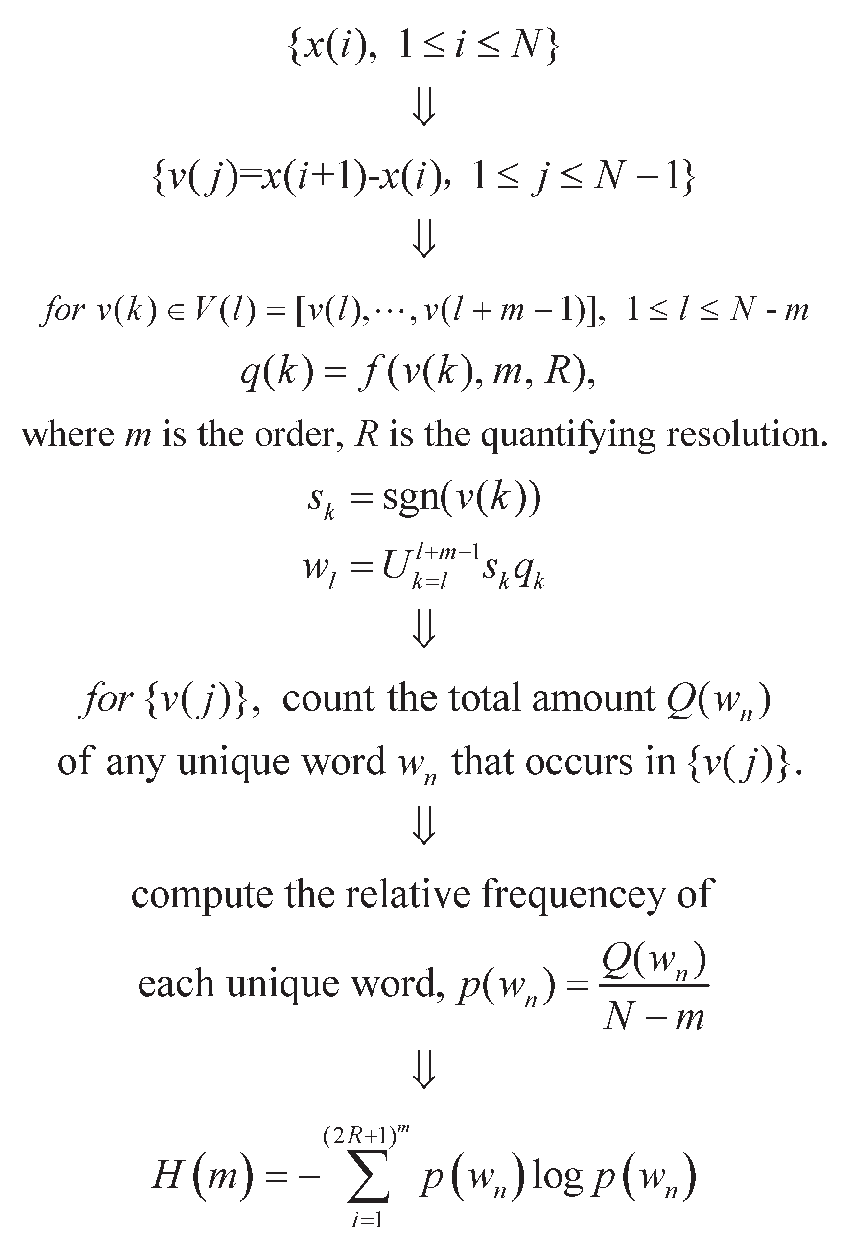
The procedure of the increment entropy is briefly summarized in Figure 1.

Figure 1. Schematic description of the steps of the increment entropy.

Figure 1. Schematic description of the steps of the increment entropy.

As usual, log is with base 2, and, thus, H is given in bit. In general, $H\left(m\right)$ is normalized by $m-1$. Obviously, $H\left(m\right)$ is bounded in $[0,mlog(2R+1\left)\right]$. For example, for a series with ten values $3,3,2,-8,-5,4,20,10,11,8$, we generate an increment sequence $0,-1,-10,3,9,16,-10,1,-3$ from the given series by a differential operator. There are a variety of ways to quantify the elements. Here, we take the order $m=2$ and the resolution level $R=4$. We quantify each element $v\left(j\right)$ in a constructed vector $V=\left\{v\right(j),j=1,\cdots ,m\}$ by the standard deviation of the vector using Equation (3). In this illustration, the magnitude of increment is quantified by the standard deviation of increment epoch and the quantifying resolution. As a result, we get eight words as shown in Table 1, any of which is unique. Correspondingly, the frequency of each word is $\frac{1}{8}$.

$$q\left(j\right)=\left\{\begin{array}{cc}0,\hfill & std\left(V\right)=0\hfill \\ min\left(R,\lfloor \frac{∥v\left(j\right)∥\times R}{std\left(V\right)}\rfloor \right),\hfill & std\left(V\right)\ne 0.\hfill \end{array}\right.$$

(3)

$$H\left(2\right)=-\frac{1}{8}log\left(\frac{1}{8}\right)\times 8=3$$

$$h\left(2\right)=\frac{H\left(2\right)}{2-1}=3$$

Table 1. Symbolization process.

Vectors			$s_1$	$q_1$	$s_2$	$q_2$
3	3	2	0	0	$-1$	4
3	2	$-8$	$-1$	0	$-1$	4
2	$-8$	$-5$	$-1$	4	1	1
$-8$	$-5$	4	1	2	1	4
$-5$	4	20	1	4	1	4
4	20	10	1	3	$-1$	2
20	10	11	$-1$	4	1	0
10	11	8	1	1	$-1$	4

Table 1. Symbolization process.

Vectors			$s_1$	$q_1$	$s_2$	$q_2$
3	3	2	0	0	$-1$	4
3	2	$-8$	$-1$	0	$-1$	4
2	$-8$	$-5$	$-1$	4	1	1
$-8$	$-5$	4	1	2	1	4
$-5$	4	20	1	4	1	4
4	20	10	1	3	$-1$	2
20	10	11	$-1$	4	1	0
10	11	8	1	1	$-1$	4

Given an epoch of m length, it could produce ${(2R+1)}^m$ possible formed patterns in IncrEn, but $m!$ patterns in PE. For smaller order m (generally less than 10), ${(2R+1)}^m$ is roughly more than $m!$. Thus, IncrEn($m,R$) could be larger than PE for random or chaotic signals, whereas it is approximate to PE for regular signals. Similar to PE, IncrEn is calculated for different embedding dimensions m. It is a theoretical problem to determine a limit for large m. In [25], Bandt and Pompe recommend $m=3,\cdots ,7$. Here, IncrEn is calculated with increment time series. A smaller data size compared to ${(2R+1)}^m$, will cause a bias in IncrEn. In practice, we recommend the order $m=2,3,4,5$. For a given m, an R can cause ${(2R+1)}^m$ possible patterns. When R is too large, IncrEn becomes over sensitive to noise. When $R=0$, the symbolization is dependent on the signs of increments, which is identical to that employed in [43]. In practical purpose, we recommend the quantifying resolution $R\le 4$.

3. Simulation and Results

We conducted simulations both on chaotic signals and regular signals (e.g., periodical signals) to examine IncrEn. We compared IncrEn with PE and SampEn on these synthetic data in various aspects, such as reliability for detecting abrupt change, data length effect, and stability.

3.1. Results on Logistic Time Series

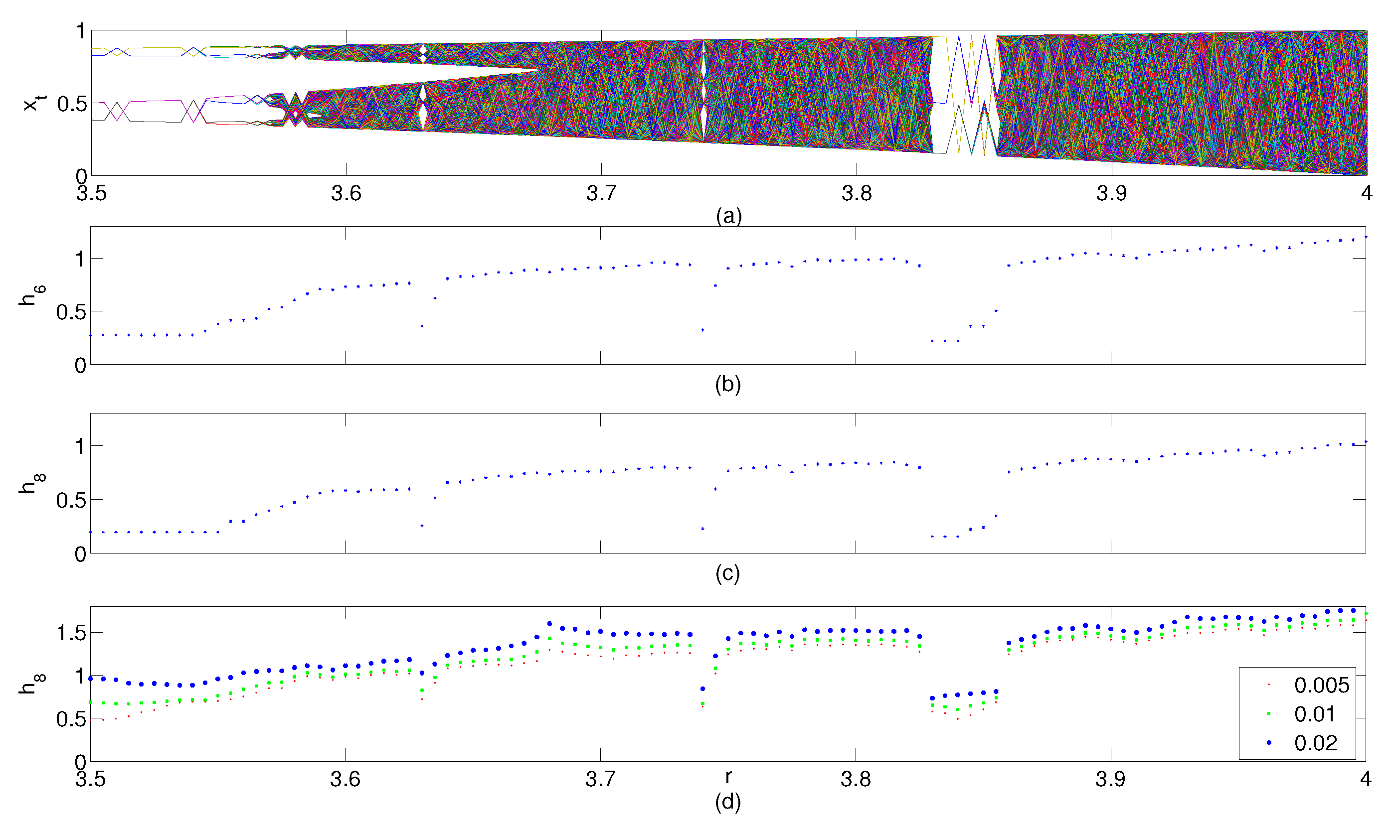
First, we demonstrate that IncrEn can effectively and accurately indicate the complexity of dynamic system using the well-known logistic map $x_n=r{x}_{n-1}(1-x_{n-1})$ already shown in previous studies [25,33]. It is well known that the behavior of the logistic map varies with the parameter r. We generated 20,000 values of the logistic map with varying control parameter r within $[3.5,4]$ and an initial value between $0.4$ and $0.6$. The bifurcation diagram of the logistic map is shown in Figure 2a. We calculate IncrEn of logistic sequence of different parameter r. IncrEn is completely consistent with the results in previous studies [25,33]. When the logistic map exhibits a periodic behavior, e.g., $r<3.56995$ (approximate), IncrEn is much lower. From almost all initial conditions, the value $x_n$ approaches permanent oscillations among four values for $3.44949<r<3.54409$ (approximately), and enters a period-doubling cascade (8, 16, 32, etc.). When r approximately approaches 3.56995, the period-doubling cascade ends and chaos starts up. For most $r>3.56995$, the sequence exhibits chaotic behavior, but, for certain ranges of r, it still shows non-chaotic behavior. For example, it oscillates among three values when r approximately approaches 3.82843, and, when r increases slightly, it oscillates among six values, then 12 values, etc. As shown in Figure 2b,c, IncrEn ($h_6$ and $h_8$) are much more sensitive to the transient instants. The functions $h_6$ and $h_8$ are quite approximate to each other. This justifies that IncrEn of a lower order is as effective as IncrEn of a higher order when being applied to real-world data [25].

We further examine the effects of Gaussian observational noise on IncrEn. Comparing Figure 2d with Figure 2c, the appearance of IncrEn is almost identical regardless of the observational noise. As shown in Figure 2d, IncrEn, $h_8$, only grows slightly, compared to that without noise, even in low-period window. This is very distinct from PE as PE is relatively larger in the low-period window, e.g., period-4 and period-3 windows (see Figure 2e in [25]).

Figure 2. Logistic equation for varying control parameter r and corresponding IncrEn with varying scale. (a) bifurcation diagram; (b) increment Entropy, $h_6$; (c) $h_8;$ (d) $h_8$ with Gaussian observational noise at standard deviations.

Figure 2. Logistic equation for varying control parameter r and corresponding IncrEn with varying scale. (a) bifurcation diagram; (b) increment Entropy, $h_6$; (c) $h_8;$ (d) $h_8$ with Gaussian observational noise at standard deviations.

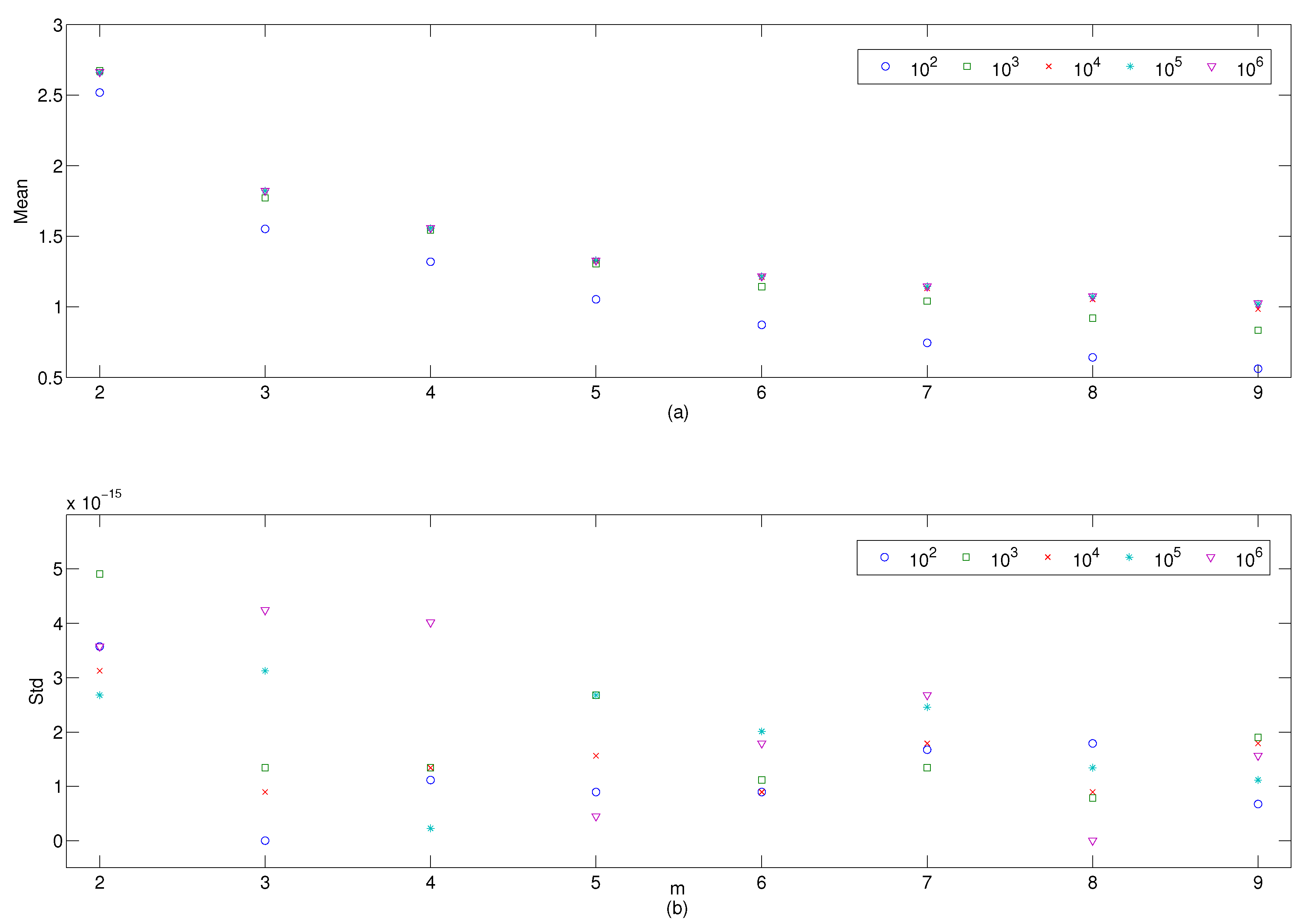
We examine the effect of data length on IncrEn. We take 100 time series with various data length. Each series is produced by the logistic map with $r=4$ and an initial value between $0.4$ and $0.6$. We calculate the IncrEn of each series with $R=4$. As shown in Figure 3a, $h_m$ decreases with m. IncrEn is very approximate when the data length is beyond ${10}^3$. The variance of $h_m$ is extremely small as shown in Figure 3b.

Figure 3. Order m choice and data length effect. (a) mean $<h_m>$ of logistic map ($r=4$) with ${10}^k$ data points ($k=2,3,4,5,6$). Horizontal: embeding dimension m; (b) corresponding standard deviation σ of $h_m$.

Figure 3. Order m choice and data length effect. (a) mean $<h_m>$ of logistic map ($r=4$) with ${10}^k$ data points ($k=2,3,4,5,6$). Horizontal: embeding dimension m; (b) corresponding standard deviation σ of $h_m$.

3.2. Relationship to Other Approaches

The primary motivation of IncrEn is to characterize the magnitude of the relative changes of the values and instants that these changes occur in time series. IncrEn combines the concepts of entropy and symbolic dynamics, which is related to PE. If the quantifying level is 0, IncrEn($m,R$) reduces into IncrEn(m), which is computed based on the sign correlation. In this case, IncrEn(m) can be considered as a variant of PE in which the values in a vector are compared with only their nearest neighbors, rather than the every element in the vector. IncrEn quantifies the diversity of possible incremental patterns of the values in a time series. We further conducted simulations to illustrate the features of IncrEn and compared IncrEn with PE and SampEn.

3.2.1. Distinguishing Analogous Patterns

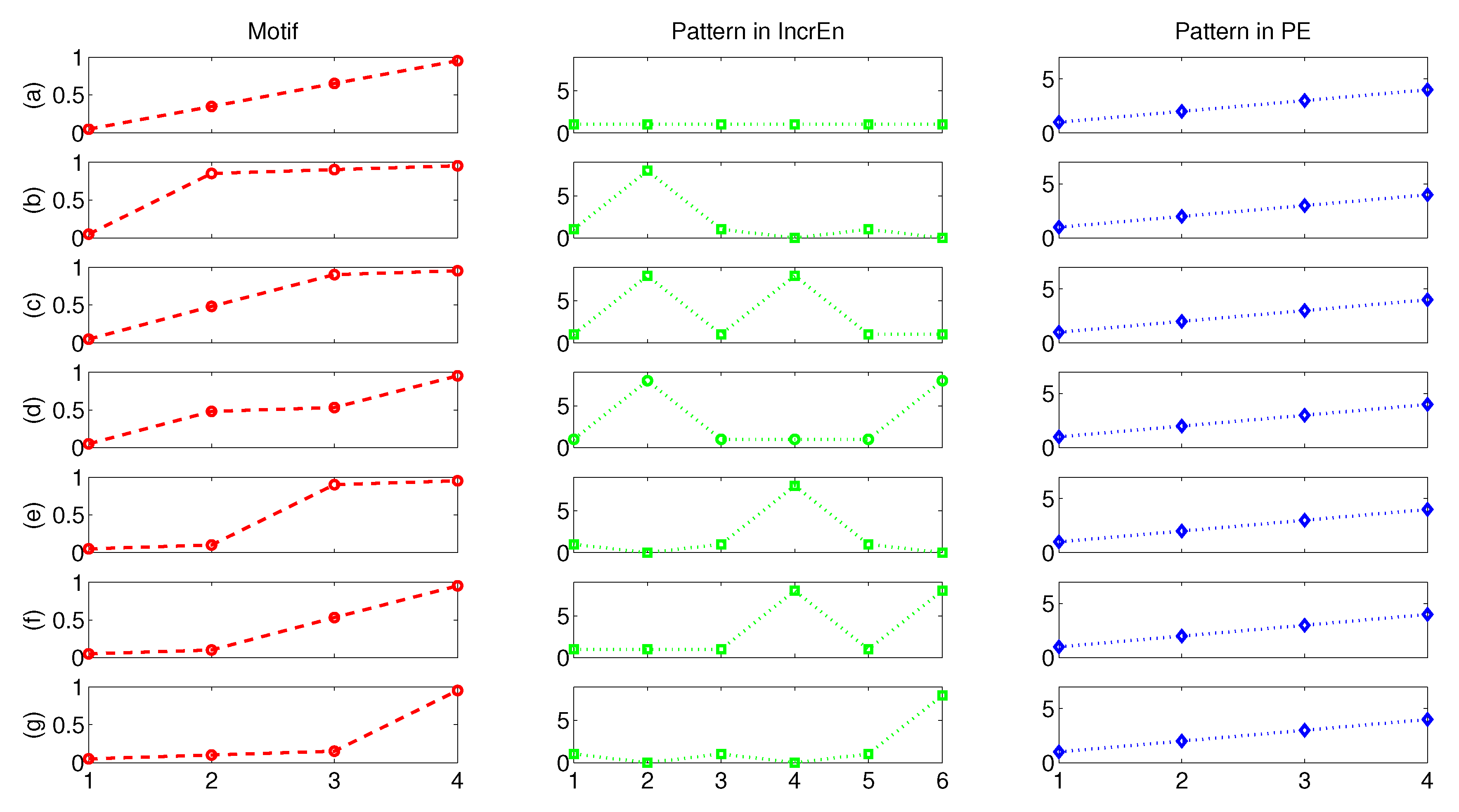
We construct a group of motifs, each of which is composed of four points in ascending order, as shown in the left panel of Figure 4. Although these motifs look similar, none of them is identical to other motifs. In IncrEn, these seven motifs are mapped into seven different patterns with order $m=3$ and quantifying resolution $R=4$, although their elements align with an identical order. However, they are transformed into an identical pattern in PE because all of them are in ascending order. This makes IncrEn more sensitive to changes hidden in time series. It is clear that the vector that forms the motif in Figure 4b is symmetrical to that in Figure 4g with respect to the vector in Figure 4a, and thus obviously their distance (e.g., Euclidean distance) to the vector in Figure 4a is equal. Therefore, those vectors with distinct appearances could not be effectively distinguished by SampEn and ApEn.

Figure 4. Analogous motifs (a–g) and their corresponding patterns in IncrEn and PE.

Figure 4. Analogous motifs (a–g) and their corresponding patterns in IncrEn and PE.

3.2.2. Detecting Energetic Change and Structural Change

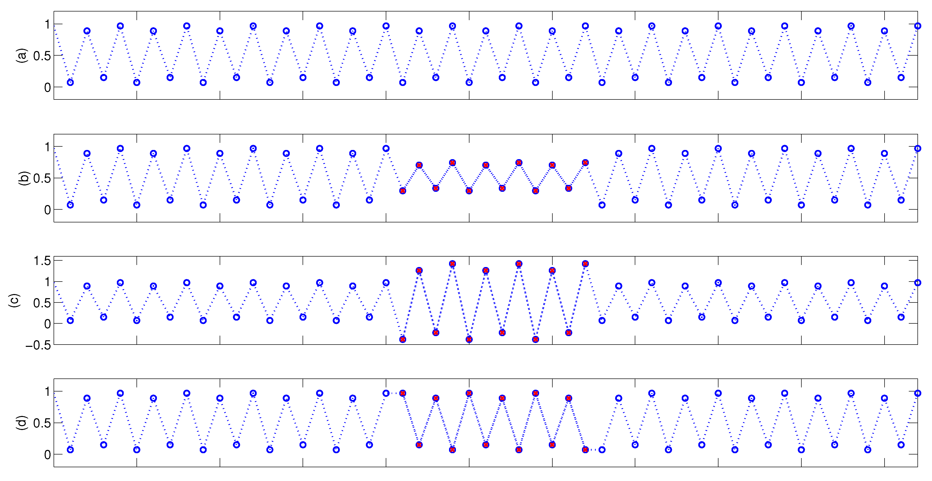
In this paper, we further examine the applications of IncrEn on detecting energetic and structural changes. The previous studies have illustrated the failure of PE for detecting abrupt change in amplitude (see Figure 1 in [33], Figure 2a in [36]). Either spike or burst in signal is one kind of energetic change in signal. We simulated three kinds of signals: regular signal, regular one interspersed with energetic mutations, and regular ones interspersed with structural mutations. We randomly generated a group of real numbers that are denoted as an atomic epoch. Then, we changed the amplitude of the atomic epoch but kept its ordinal pattern to construct an energetic mutation epoch. Likewise, a structural mutation epoch can be easily produced only by permuting the elements of the atomic epoch in reverse. A regular signal is produced by replicating the atomic epoch hundreds of times (see Figure 5a). Here, the atomic epoch is four random real numbers, and the energetic mutation is produced by multiplying it by a factor $\sqrt{2}$, and the structural mutation is produced by reversing its order. A regular signal is composed of 300 atomic epochs. Signals with energetic or structural change are composed of a large number of atomic epochs and a few mutation epochs. In Figure 5, we illustrated a group of simulated signals. We ran the simulation for 300 times. We computed IncrEn, PE, and SampEn on resultant data using various parameters ($R=4,m=2,3,4$ for IncrEn; $m=2,3,4$ for PE; $r=0.2std,m=2,3,4$ for SampEn). We also calculated IncrEn with other quantifying resolution R ($R\le 3$) and obtain the similar results.

IncrEn, PE, and SampEn of each signal are presented in Table 2 (Mean ± std). SampEn for all signals presented in Figure 5 is equal to zero, which indicates that SampEn can hardly differentiate the signals with a few mutations from the original regular signal. SampEn fails to detect the subtle change, either energetic or structural. When the order is lower, $m=2,3$, PE for signals with energetic changes is almost equal to that for the original signal ($p>0.05$ for $m=2$; $p>0.05$ for $m=3$). PE is a little larger for signals with structural mutations than that for original signal. However, it is not significant, ($p>0.05$ for $m=2$; $p>0.05$ for $m=3$). When the order becomes higher, $m=4$, PE is larger for signals with energetic mutations ($0.4611\pm 0.0031$) than the original regular signal ($0.4600\pm 0$), $p<0.0001$. Similarly, PE is quite larger for signals with structural mutations ($0.4766\pm 0.0048$) than the original regular signal, $p<0.0001$. IncrEn is significantly larger for signals with energetic mutations ($0.4698\pm 0.0014$) than the original regular ones ($0.4600\pm 0$) at the order $m=4$ ($p<0.0001$). It is also much larger for signals with structural mutations ($0.4788\pm 0.0033$) than the original one at the order $m=4$ ($p<0.0001$). At the order $m=3$, IncrEn performs better than PE and SampEn, because both PE and SampEn can capture only structural mutations, $p=0.0004$. IncrEn is more sensitive to a fraction of subtle structural changes than both PE and SampEn. At the order $m=4$, both IncrEn and PE are significantly larger for signals with structural mutation than those with energetic mutation, $p<0.0001$ for both. It indicates that both of them are capable of distinguishing structural mutation from energetic mutations.

Figure 5. Detection of energetic and structual change. (a) Regular time series consists of 300 identical atomic epochs that contain four random numbers; (b) Time series interspersed with three energetic mutation epochs (attenuation); (c) Time series interspersed with three energetic mutation epochs (enhancement); (d) Time series interspersed with three structural mutation epochs.

Figure 5. Detection of energetic and structual change. (a) Regular time series consists of 300 identical atomic epochs that contain four random numbers; (b) Time series interspersed with three energetic mutation epochs (attenuation); (c) Time series interspersed with three energetic mutation epochs (enhancement); (d) Time series interspersed with three structural mutation epochs.

Table 2. Increment entropy (IncrEn), permutation entropy (PE), and sample entropy (SampEn) of regular signals, regular ones with energetic mutations, and regular ones with structural mutations.

Entropy		Regular	Energetic Mutation	Structural Mutation
IncrEn	$m=2$	1.3235 ± 0.1380	1.3264 ± 0.1372	1.3529 ± 0.1378
	$m=3$	0.6849 ± 0.0379	0.6937 ± 0.0387	0.7044 ± 0.0388
	$m=4$	0.4600 ± 0.0000	0.4698 ± 0.0014	0.4788 ± 0.0033
PE	$m=2$	0.6367 ± 0.0643	0.6367 ± 0.0643	0.6386 ± 0.0621
	$m=3$	0.6271 ± 0.0825	0.6275 ± 0.0828	0.6397 ± 0.0791
	$m=4$	0.4600 ± 0.0000	0.4611 ± 0.0031	0.4788 ± 0.0033
SampEn	$m=2$	0.0082 ± 0.0577	0.0083 ± 0.0577	0.0082 ± 0.0577
	$m=3$	0.0000 ± 0.0000	0.0000 ± 0.0000	0.0000 ± 0.0000
	$m=4$	0.0000 ± 0.0000	0.0000 ± 0.0000	0.0000 ± 0.0000

Table 2. Increment entropy (IncrEn), permutation entropy (PE), and sample entropy (SampEn) of regular signals, regular ones with energetic mutations, and regular ones with structural mutations.

Entropy		Regular	Energetic Mutation	Structural Mutation
IncrEn	$m=2$	1.3235 ± 0.1380	1.3264 ± 0.1372	1.3529 ± 0.1378
	$m=3$	0.6849 ± 0.0379	0.6937 ± 0.0387	0.7044 ± 0.0388
	$m=4$	0.4600 ± 0.0000	0.4698 ± 0.0014	0.4788 ± 0.0033
PE	$m=2$	0.6367 ± 0.0643	0.6367 ± 0.0643	0.6386 ± 0.0621
	$m=3$	0.6271 ± 0.0825	0.6275 ± 0.0828	0.6397 ± 0.0791
	$m=4$	0.4600 ± 0.0000	0.4611 ± 0.0031	0.4788 ± 0.0033
SampEn	$m=2$	0.0082 ± 0.0577	0.0083 ± 0.0577	0.0082 ± 0.0577
	$m=3$	0.0000 ± 0.0000	0.0000 ± 0.0000	0.0000 ± 0.0000
	$m=4$	0.0000 ± 0.0000	0.0000 ± 0.0000	0.0000 ± 0.0000

3.2.3. Invariance of IncrEn

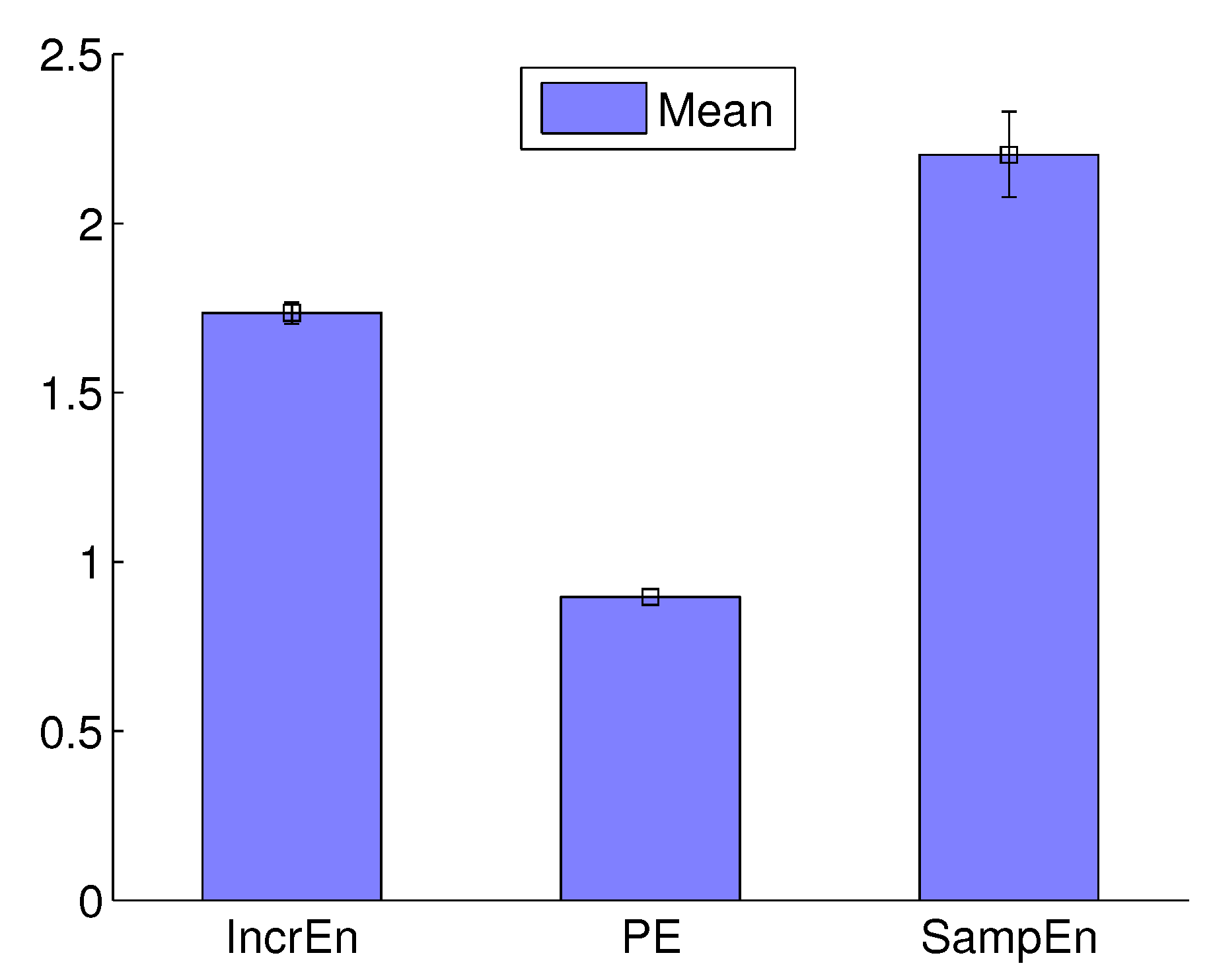
We address the invariance of IncrEn on a random Gaussian noise series. Here, we simulated 200 Gaussian noise series of 10,000 points. We calcuated IncrEn of an epoch of 1000 points truncated from each series. As shown in Figure 6, the standard deviation of IncrEn is quite small, 0.0319, compared with SampEn, 0.1268. PE is almost a constant because the standard deviation is extremely small—0.0006. In terms of the invariance, IncrEn is better than SampEn but inferior to PE.

Figure 6. Invariance of IncrEn, PE and SampEn on random noise.

Figure 6. Invariance of IncrEn, PE and SampEn on random noise.

3.3. Application to Seizure Detection from EEG Signals

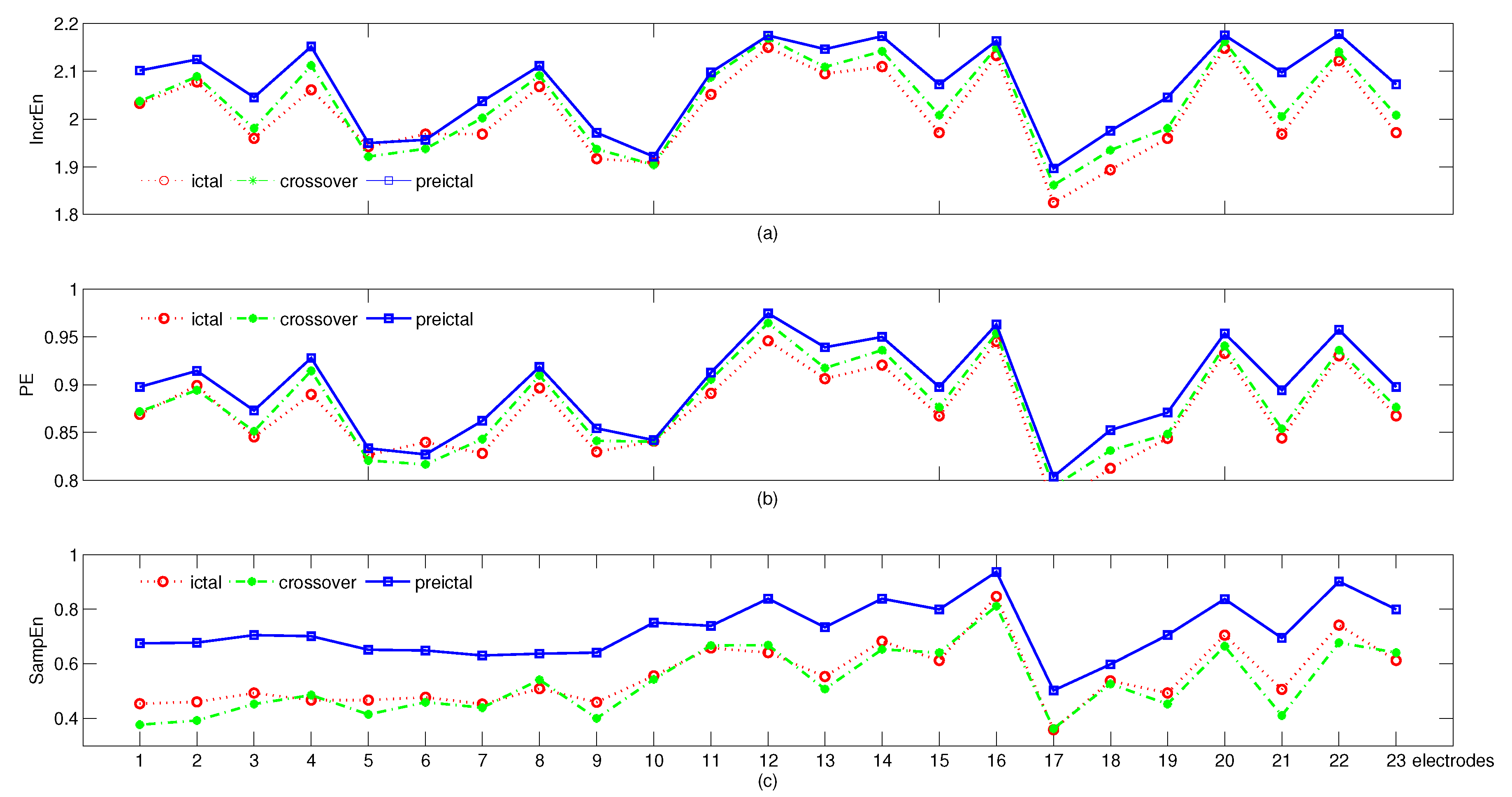
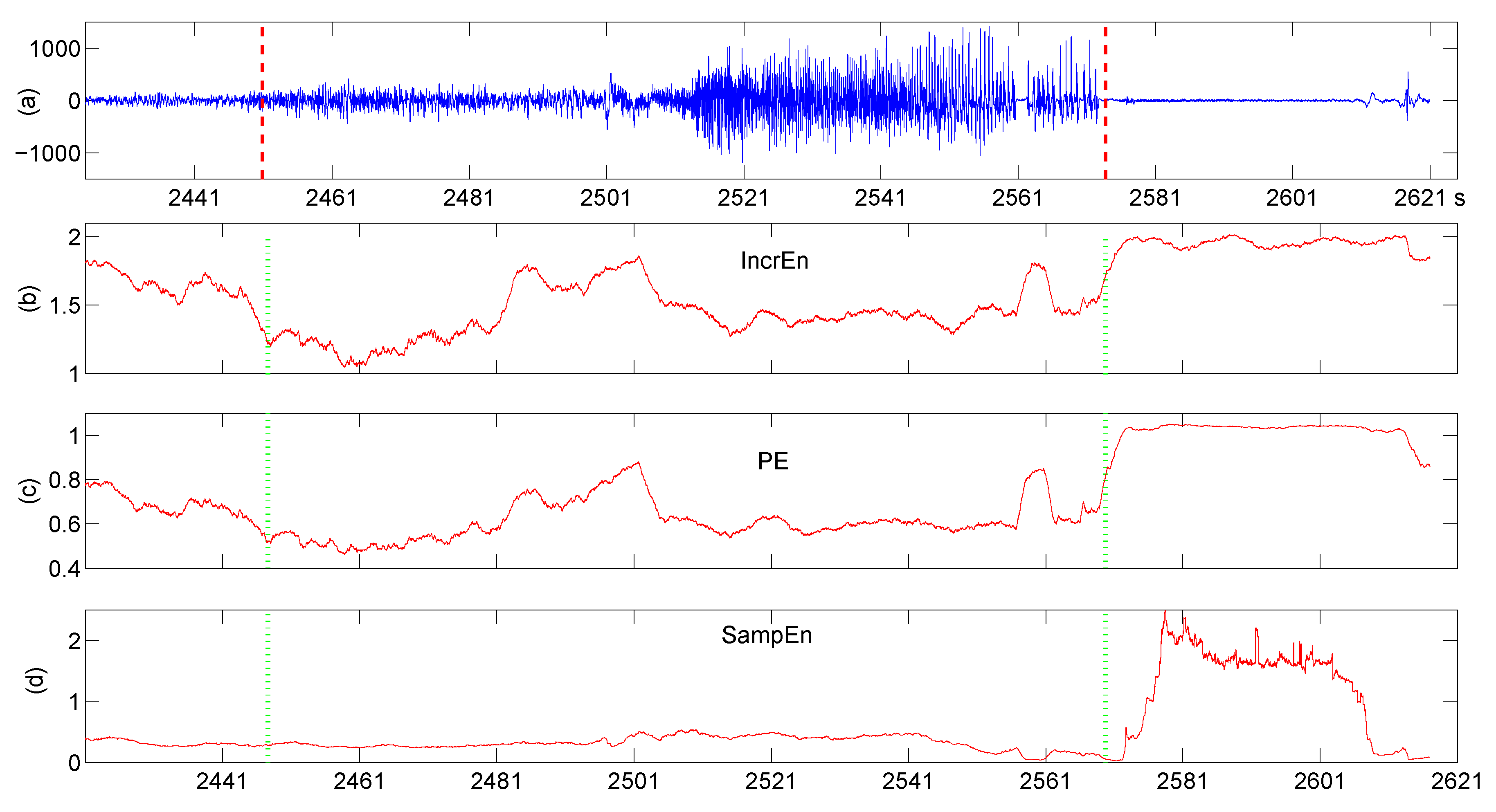
Entropy has been an effective approach to be used to detect seizure from EEG signals [27,33,36]. In this section, we demonstrate our proposed IncrEn on the detection of epileptic EEGs that contain a seizure and compare it with PE and SampEn. Here, the dataset used to evaluate our proposed IncrEn is from the CHB-MIT scalp EEG database that is freely available online [44,45,46]. EEG recordings in the data sets were recorded from 23 pediatric patients (five males, ages 3.5–22, 18 females, ages 1.5–19) at the Children’s Hospital Boston. The continuous scalp EEG were sampled at 256 Hz. The clinical seizures in the EEG recordings are identified by experts and are annotated the onset and the end. The data were segmented into one hour long records, and 14 seizure records that contain one or more seizures are used in the experiment, seven seizure records of subject 1 (female, aged 11), and seven seizure records of subject 3 (female, aged 14). We compute IncrEn ($m=4,R=4$) of three epochs of each seizure record to check if IncrEn is capable of identifying a seizure, one right before the seizure onset (preictal), one right after the seizure onset (ictal), and a crossover that contains a part of seizure (crossover). IncrEn becomes lower from the preictal stage to the ictal stage. This is consistent with previous studies that entropy decreases during the seizure stage and increases when the seizure ends [33,47]. The average of IncrEn at preictal stage over 14 data sets is the largest over most of electrodes, and that at the ictal stage is the second largest over most of electrodes. That at the crossover stage is the least over most of electrodes, as presented in Figure 7a. The differences among them are not significant over all the electrodes ($p>0.005$). PE is similar to IncrEn, as shown in Figure 7b. Likewise, the differences among the three stages are not significant over all the electrodes ($p>0.005$). Similarly, the average of SampEn at preictal stage over 14 datasets are significantly larger than those at other stages over several electrodes. Unlike both IncrEn and PE, the differences of the average of SampEn over 14 datasets between the crossover stage and ictal stage are erratic over the electrodes, see Figure 7c. We use a sliding window on a seizure record to illustrate that IncrEn is able to detect the seizure onset, a change point of time series. Here, we further calculated IncrEn with various parameters of the seizure record using a window size of 500 samples with 499 samples overlapped. Here, we showed IncrEn ($m=4,R=4$), PE ($m=4$) and SampEn ($m=4,r=0.2std$) in Figure 8. IncrEn is more sensitive to the seizure onset. It goes downwards obviously at the initial phase of seizure and upwards at the end of seizure. Further, from Figure 8b IncrEn is sensitive to the transient amplitude changes within the seizure record. We also calculated IncrEn, PE, and SampEn with different parameters, and found similar results to that in Figure 8.

Figure 7. Average of IncrEn (a); PE (b); and SampEn (c) over 14 epileptic EEG signals at preictal, crossover, and ictal stages.

Figure 7. Average of IncrEn (a); PE (b); and SampEn (c) over 14 epileptic EEG signals at preictal, crossover, and ictal stages.

Figure 8. Detecting the seizure onset in a seizure record (a); using IncrEn (b); PE (c); and SampEn (d). The left vertical dashed line denotes the seizure onset, and the right vertical dashed line denotes the end of seizure.

Figure 8. Detecting the seizure onset in a seizure record (a); using IncrEn (b); PE (c); and SampEn (d). The left vertical dashed line denotes the seizure onset, and the right vertical dashed line denotes the end of seizure.

3.4. Application to Bearing Fault Detection by Vibration

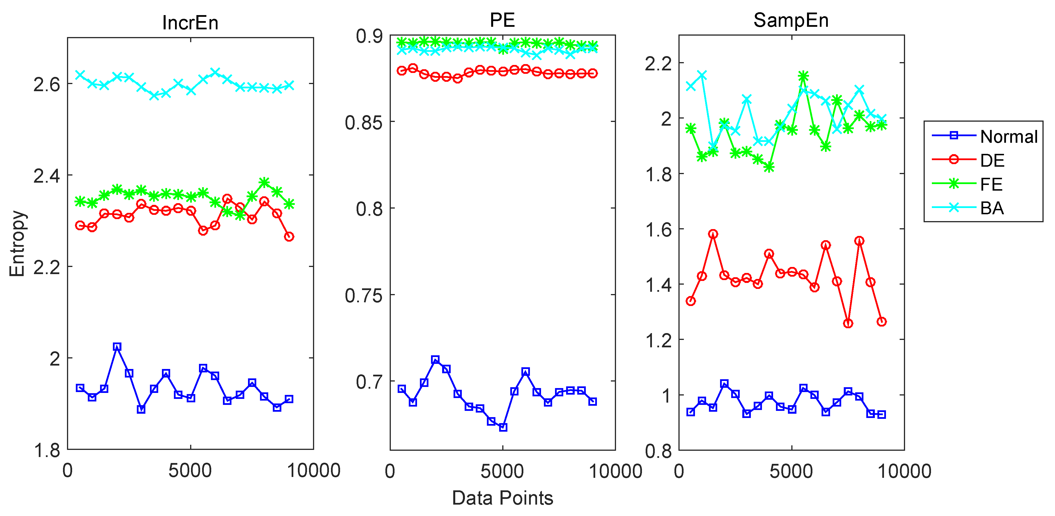
In this section, we demonstrate the detection of rolling bearing fault using IncrEn. Vibration based bearing fault detection has been broadly applied in practice. Researchers and engineers often use nonlinear analysis to extract the nonlinear feature of vibration related to the faults, such as the correlation dimension, the largest Lyapunov exponent, and entropy. Because PE based approaches have been used to diagnose bearing fault, we use IncrEn to analyze bearing fault data that are available at the Case Western Reserve University bearing data center [48]. Motor bearings faults range from 0.007 inches to 0.040 inches in diameter, which were located separately at the inner raceway, rolling element (i.e., ball) and outer raceway. Tri-axis accelerometers mounted at the 12 o’clock position at both the drive end and fan end of the motor housing were utilized to collect vibration data was collected using accelerometers at 12,000 samples per second (see more details of data description from the Case Western Reserve University bearing data center). In order to exhibit the performance of IncrEn of various parameters, we compute IncrEn with $m=3$, $R=3$, and $N=1000$ for four kinds of vibration acceleration signals recorded on a bearing with fault of 0.007 inches at rolling element (ball). One signal is a normal baseline (0 hp motor load, 1797 rpm motor speed), and the other three signals are from sensors equipped on different positions including the drive end (DE), the fan end (FE), the motor supporting base plate (BA). We also compute PE with $m=3$ and $N=1000$ and SampEn with $m=3$ and $r=0.2std$ for these signals. Results are presented in Figure 9. IncrEn of three fault vibration signals (DE, FE, and BA) are significantly larger than the normal baseline signal (p < 0.001). Similarly, both PE and SampEn are significantly larger than the normal baseline signal (p < 0.0001). It is hard for PE to discriminate the fault vibration under BA and FE conditions, and it is also difficult for SampEn. IncrEn performs well for detecting the fault vibration signals.

Figure 9. IncrEn, PE and SampEn of vibration acceleration signals recorded on a bearing with a fault on rolling element. A sliding time window of 1000 samples with 500 overlapped samples is adopted.

Figure 9. IncrEn, PE and SampEn of vibration acceleration signals recorded on a bearing with a fault on rolling element. A sliding time window of 1000 samples with 500 overlapped samples is adopted.

4. Discussion

There are various measures of complexity of time series. Most of measures of complexity monotonically increase with randomness, giving a lower value for regular sequences but a higher one for random sequences. Other definitions assign a lower value for both completely regular and pure random sequences but a higher one for the intermediate stage [18,49,50,51]. However, from the point of view of predictability, neither chaotic sequence nor random sequence is predictable. Both of them are highly complex [13]. Our approach is an intuitive notion of complexity in that IncrEn grows up with increasing disorder, maximizing at random stage but minimizing at regular stage. On this respect, it is the same as PE and SampEn. IncrEn is lower for a regular sequence, higher for a random one, and intermediate for a chaotic one. Thus, it is a measure of the degree of predictability.

Our simulation has demonstrated that IncrEn is more sensitive not only to a subtle alternation of amplitude but also to a tiny modification of structure, as shown in Figure 3 and Figure 4. This allows it to accurately capture subtle changes hidden in sequences, either energetic or structural. As a result, IncrEn can be used to extract various features hidden in time series and to detect dynamical change in time series caused by internal or external factors.

In recent years, entropy has been an effective method to characterize and to distinguish the physiological signals across diverse physiological and pathological conditions, such as HRV abnormality [20,21], neural disorder [22,52,53], gaits analysis [23], etc. As shown in Figure 7 and Figure 8, IncrEn exhibits better performance on seizure detection from real epileptic EEG signals than PE and SampEn. A prominent merit of IncrEn lies in that the computation of IncrEn does not make any assumption on data, which makes it applicable to diverse signals. In particular, it is an appropriate measure to examine the characteristics of those signals consisting of some equal values, e.g., HRV, which is not considered by PE [25,37]. IncrEn exhibits robustness to observational noise. As shown in Figure 2d, noise does not disturb appearance of IncrEn, even in a shorter-period window. Noise only causes a slight increase in IncrEn. IncrEn is robust against noise (comparing Figure 2d).

The previous studies have shown that the data length has impact on the entropy computation [8,16,24,25,54]. Even for a shorter data length, e.g., 100, the variance of IncrEn across different data lengths is small as shown in Figure 3. This indicates that IncrEn is a powerful tool for analyzing very short signals. In addition, both IncrEn and PE have quite good invariance when being applied to Gaussian noise sequence. In contrast, SampEn of Gaussian noise sequences fluctuates violently as shown in Figure 6.

5. Conclusions

In this paper, we present the notion of IncrEn that is a novel measure to quantify the complexity of time series. The symbolization of IncrEn considers both the magnitude and sign of the increments constructed from time series. Results of a group of simulations and experiments on real data have indicated that IncrEn can be applied to reveal the characteristics of a variety of signals and to discriminate sequences across various conditions. Our approach possesses merits of change detection of time series. It is a promising method to characterize time series of diverse fields.

References

1. Hornero, R.; Abasolo, D.; Jimeno, N.; Sanchez, C.I.; Poza, J.; Aboy, M. Variability, regularity, and complexity of time series generated by schizophrenic patients and control subjects. IEEE Trans. Biomed. Eng. 2006, 53, 210–218. [Google Scholar] [CrossRef] [PubMed]
2. Gonzalez Andino, S.L.; Grave de Peralta Menendez, R.; Thut, G.; Spinelli, L.; Blanke, O.; Michel, C.M.; Landis, T. Measuring the complexity of time series: An application to neurophysiological signals. Hum. Brain Mapp. 2000, 11, 46–57. [Google Scholar] [CrossRef]
3. Friston, K.J.; Tononi, G.; Sporns, O.; Edelman, G.M. Characterising the complexity of neuronal interactions. Hum. Brain Mapp. 1995, 3, 302–314. [Google Scholar] [CrossRef]
4. Zamora-López, G.; Russo, E.; Gleiser, P.M.; Zhou, C.; Kurths, J. Characterizing the complexity of brain and mind networks. Philos. Trans. R. Soc. Lond. A 2011, 369, 3730–3747. [Google Scholar] [CrossRef] [PubMed]
5. Olbrich, E.; Achermann, P.; Wennekers, T. The sleeping brain as a complex system. Philos. Trans. R. Soc. Lond. A 2011, 369, 3697–3707. [Google Scholar] [CrossRef] [PubMed]
6. Costa, M.; Goldberger, A.L.; Peng, C.K. Multiscale Entropy Analysis of Complex Physiologic Time Series. Phys. Rev. Lett. 2002, 89, 068102. [Google Scholar] [CrossRef] [PubMed]
7. Pincus, S.M.; Goldberger, A.L. Physiological time-series analysis: What does regularity quantify? Am. J. Physiol. 1994, 266, H1643–H1656. [Google Scholar] [PubMed]
8. Richman, J.S.; Moorman, J.R. Physiological time-series analysis using approximate entropy and sample entropy. Am. J. Physiol. 2000, 278, H2039–H2049. [Google Scholar]
9. Tononi, G.; Sporns, O.; Edelman, G.M. A measure for brain complexity: Relating functional segregation and integration in the nervous system. Proc. Natl. Acad. Sci. USA 1994, 91, 5033–5037. [Google Scholar] [CrossRef] [PubMed]
10. Barnett, W.A.; Medio, A.; Serletis, A. Nonlinear and Complex Dynamics in Economics. Available online: http://econwpa.repec.org/eps/em/papers/9709/9709001.pdf (accessed on 8 January 2016).
11. Arthur, W.B. Complexity and the Economy. Science 1999, 284, 107–109. [Google Scholar] [CrossRef] [PubMed]
12. Turchin, P.; Taylor, A.D. Complex Dynamics in Ecological Time Series. Ecology 1992, 73, 289–305. [Google Scholar] [CrossRef]
13. Boffetta, G.; Cencini, M.; Falcioni, M.; Vulpiani, A. Predictability: A way to characterize complexity. Phys. Rep. 2002, 356, 367–474. [Google Scholar] [CrossRef]
14. Lempel, A.; Ziv, J. On the Complexity of Finite Sequences. IEEE Trans. Inf. Theory 1976, 22, 75–81. [Google Scholar] [CrossRef]
15. Kolmogorov, A. Logical basis for information theory and probability theory. IEEE Trans. Inf. Theory 1968, 14, 662–664. [Google Scholar] [CrossRef]
16. Pincus, S.M. Approximate entropy as a measure of system complexity. Proc Natl. Acad. Sci. USA 1991, 88, 2297–2301. [Google Scholar] [CrossRef] [PubMed]
17. Crutchfield, J.P.; Young, K. Inferring statistical complexity. Phys. Rev. Lett. 1989, 63, 105–108. [Google Scholar] [CrossRef] [PubMed]
18. Shiner, J.S.; Davison, M.; Landsberg, P.T. Simple measure for complexity. Phys. Rev. E 1999, 59, 1459–1464. [Google Scholar] [CrossRef]
19. Pincus, S.M.; Goldberger, A.L. Physiological time-series analysis: What does regularity quantify? Am. J. Physiol. 1994, 266, H1643–H1656. [Google Scholar] [PubMed]
20. Porta, A.; Guzzetti, S.; Furlan, R.; Gnecchi-Ruscone, T.; Montano, N.; Malliani, A. Complexity and nonlinearity in short-term heart period variability: Comparison of methods based on local nonlinear prediction. IEEE Trans. Biomed. Eng. 2007, 54, 94–106. [Google Scholar] [CrossRef] [PubMed]
21. Lake, D.E.; Richman, J.S.; Griffin, M.P.; Moorman, J.R. Sample entropy analysis of neonatal heart rate variability. Am. J. Physiol. 2002, 283, R789–R797. [Google Scholar] [CrossRef] [PubMed]
22. Takahashi, T.; Cho, R.Y.; Mizuno, T.; Kikuchi, M.; Murata, T.; Takahashi, K.; Wada, Y. Antipsychotics reverse abnormal EEG complexity in drug-naive schizophrenia: A multiscale entropy analysis. NeuroImage 2010, 51, 173–182. [Google Scholar] [CrossRef] [PubMed]
23. Buzzi, U.H.; Ulrich, B.D. Dynamic stability of gait cycles as a function of speed and system constraints. Mot. Control 2004, 8, 241–254. [Google Scholar]
24. Yentes, J.; Hunt, N.; Schmid, K.; Kaipust, J.; McGrath, D.; Stergiou, N. The Appropriate Use of Approximate Entropy and Sample Entropy with Short Data Sets. Ann. Biomed. Eng. 2013, 41, 349–365. [Google Scholar] [CrossRef] [PubMed]
25. Bandt, C.; Pompe, B. Permutation Entropy: A Natural Complexity Measure for Time Series. Phys. Rev. Lett. 2002, 88, 174102. [Google Scholar] [CrossRef] [PubMed]
26. Bandt, C.; Keller, G.; Pompe, B. Entropy of interval maps via permutations. Nonlinearity 2002, 15, 1595–1602. [Google Scholar] [CrossRef]
27. Cao, Y.; Tung, W.W.; Gao, J.; Protopopescu, V.; Hively, L. Detecting dynamical changes in time series using the permutation entropy. Phys. Rev. E 2004, 70, 046217. [Google Scholar] [CrossRef] [PubMed]
28. Xu, X.; Zhang, J.; Small, M. Superfamily phenomena and motifs of networks induced from time series. Proc. Natl. Acad. Sci. USA 2008, 105, 19601–19605. [Google Scholar] [CrossRef] [PubMed]
29. Staniek, M.; Lehnertz, K. Symbolic transfer entropy. Phys. Rev. Lett. 2008, 100, 158101. [Google Scholar] [CrossRef] [PubMed]
30. Olofsen, E.; Sleigh, J.; Dahan, A. Permutation entropy of the electroencephalogram: A measure of anaesthetic drug effect. Br. J. Anaesth. 2008, 101, 810–821. [Google Scholar] [CrossRef] [PubMed]
31. Zunino, L.; Zanin, M.; Tabak, B.M.; Pérez, D.G.; Rosso, O.A. Forbidden patterns, permutation entropy and stock market inefficiency. Physica A 2009, 388, 2854–2864. [Google Scholar] [CrossRef]
32. Hornero, R.; Abásolo, D.; Escudero, J.; Gómez, C. Nonlinear analysis of electroencephalogram and magnetoencephalogram recordings in patients with Alzheimer’s disease. Philos. Trans. R. Soc. A 2009, 367, 317–336. [Google Scholar] [CrossRef] [PubMed] [Green Version]
33. Liu, X.F.; Wang, Y. Fine-grained permutation entropy as a measure of natural complexity for time series. Chin. Phys. B 2009, 18, 2690–2695. [Google Scholar]
34. Ruiz, M.D.C.; Guillamón, A.; Gabaldón, A. A new approach to measure volatility in energy markets. Entropy 2012, 14, 74–91. [Google Scholar] [CrossRef]
35. Zanin, M.; Zunino, L.; Rosso, O.A.; Papo, D. Permutation entropy and its main biomedical and econophysics applications: A review. Entropy 2012, 14, 1553–1577. [Google Scholar] [CrossRef]
36. Fadlallah, B.; Chen, B.; Keil, A.; Principe, J. Weighted-permutation entropy: A complexity measure for time series incorporating amplitude information. Phys. Rev. E 2013, 87, 022911. [Google Scholar] [CrossRef] [PubMed]
37. Bian, C.; Qin, C.; Ma, Q.D.; Shen, Q. Modified permutation-entropy analysis of heartbeat dynamics. Phys. Rev. E 2012, 85, 021906. [Google Scholar] [CrossRef] [PubMed]
38. Liu, X.F.; Yu, W.L. A symbolic dynamics approach to the complexity analysis of event-related potentials. Acta Phys. Sin. 2008, 57, 2587–2594. [Google Scholar]
39. Daw, C.S.; Finney, C.E.A.; Tracy, E.R. A review of symbolic analysis of experimental data. Rev. Sci. Instrum. 2003, 74, 915–930. [Google Scholar] [CrossRef]
40. Marston, M.; Hedlund, G.A. Symbolic Dynamics. Am. J. Math. 1938, 60, 815–866. [Google Scholar]
41. Marston, M.; Hedlund, G.A. Symbolic Dynamics II. Sturmian Trajectories. Am. J. Math. 1940, 62, 1–42. [Google Scholar] [CrossRef]
42. Graben, P.B.; Saddy, J.D.; Schlesewsky, M.; Kurths, J. Symbolic dynamics of event-related brain potentials. Phys. Rev. E 2000, 62, 5518–5541. [Google Scholar] [CrossRef]
43. Ashkenazy, Y.; Ivanov, P.; Havlin, S.; Peng, C.; Goldberger, A.; Stanley, E. Magnitude and sign correlations in heartbeat fluctuations. Phys. Rev. Lett. 2001, 86, 1900–1903. [Google Scholar] [CrossRef] [PubMed]
44. CHB-MIT Scalp EEG Database. Available online: http://www.physionet.org/pn6/chbmit/ (accessed on 8 January 2016).
45. Shoeb, A.; Edwards, H.; Connolly, J.; Bourgeois, B.; Ted Treves, S.; Guttag, J. Patient-specific seizure onset detection. Epilepsy Behav. 2004, 5, 483–498. [Google Scholar] [CrossRef] [PubMed]
46. Shoeb, A.H.; Guttag, J.V. Application of machine learning to epileptic seizure detection. In Proceedings of the 27th International Conference on Machine Learning (ICML-10), Haifa, Israel, 21–24 June 2010; pp. 975–982.
47. Diambra, L.; de Figueiredo, J.C.B.; Malta, C.P. Epileptic activity recognition in EEG recording. Phys. A Stat. Mech. Appl. 1999, 273, 495–505. [Google Scholar] [CrossRef]
48. Bearing Data Center. Available online: http://csegroups.case.edu/bearingdatacenter/home (accessed on 8 January 2016).
49. Ke, D.-G. Unifying Complexity and Information. Sci. Rep. 2013, 3. [Google Scholar] [CrossRef] [PubMed]
50. Grassberger, P. Toward a quantitative theory of self-generated complexity. Int. J. Theor. Phys. 1986, 25, 907–938. [Google Scholar] [CrossRef]
51. Crutchfield, J.P. Between order and chaos. Nat. Phys. 2012, 8, 17–24. [Google Scholar] [CrossRef]
52. Srinivasan, V.; Eswaran, C.; Sriraam, N. Approximate Entropy-Based Epileptic EEG Detection Using Artificial Neural Networks. IEEE Trans. Inf. Technol. Biomed. 2007, 11, 288–295. [Google Scholar] [CrossRef] [PubMed]
53. Kannathal, N.; Choo, M.L.; Acharya, U.R.; Sadasivan, P. Entropies for detection of epilepsy in EEG. Comput. Methods Programs Biomed. 2005, 80, 187–194. [Google Scholar] [CrossRef] [PubMed]
54. Lesne, A.; Blanc, J.L.; Pezard, L. Entropy estimation of very short symbolic sequences. Phys. Rev. E 2009, 79, 046208. [Google Scholar] [CrossRef] [PubMed]