


Abstract
In this paper, a proposed computational method referred to as Projected Differential Transformation Method (PDTM) resulting from the modification of the classical Differential Transformation Method (DTM) is applied, for the first time, to the Black–Scholes Equation for European Option Valuation. The results obtained converge faster to their associated exact solution form; these easily computed results represent the analytical values of the associated European call options, and the same algorithm can be followed for European put options. It is shown that PDTM is more efficient, reliable and better than the classical DTM and other semi-analytical methods since less computational work is involved. Hence, it is strongly recommended for both linear and nonlinear stochastic differential equations (SDEs) encountered in financial mathematics.
Keywords:
analytical solution; Black–Scholes model; projected differential transform method; option valuation; European options; stochastic differential equations Mathematics Subject Classification:
35A20; 35R60; 91B70
1. Introduction
Pricing of options is a key aspect of financial mathematics and financial engineering. In 1973 Black and Scholes derived the most famous and significant valuation model, known as Black–Scholes Model for options [1]. The model is used for European or American options—be it a call option or a put option. The model is based on some assumptions, among such are the no–arbitrage opportunities, no inclusion of transaction costs associated with hedging, the asset price is lognormally distributed, the drift and the volatility rates are assumed constants, trading of all securities and derivatives are assumed continuous [2]. The assumption of the volatility as a constant function has really posed a challenge in option valuation using the Black–Scholes Model, since it is not the case in reality.
In a bid to address parts of the challenges posed by the aforementioned assumptions, many researchers have resorted to different approaches and modified models. Among these are the inclusion of jumps or stochastic parameters such as volatility in the price processes of option, Levy processes [3,4], the derivative of a no arbitrage determinant theorem for Liu’s stock model in uncertain markets [5], models driven by uncertain processes for option pricing [6,7,8] and so on.
We remark here that the market value of a call option is a function of the underlying asset price, the exercise price, interest rate, expiration time, and the stock volatility . Despite these shortcomings, the Black–Scholes Model remains the hallmark of option pricing models for derivative security, and still proves very useful and vital both empirically and theoretically for the following reasons: the price of the option does not explicitly rely on the preferences of investors—risk –neutral valuation relationship (RNVR. Therefore, there is a greater need for better semi-analytical methods for solutions of such models resulting from stochastic differential equations (SDEs) and uncertain differential equations (UDEs).
In what follows, we will consider the classical celebrated Black–Scholes option pricing model:
where is the value of the contingent claim , at time, , , with a payoff function , and expiration price, such that:
where indicates the large value between and 0.
Theorem 1.
[One-dimensional Ito formula] [9,10]
For an adapted stochastic process , satisfying the stochastic differential equation (SDE):
we have:
where .
For the derivation of Equation (1), Theorem 1 is applied (see [11] and the references therein for other necessary details). We remark here that Equation (1) holds for options whose underlying stock do not pay dividends provided that , and upon the satisfaction of the assumptions associated with the Black–Scholes model.
Many researchers and authors have attempted to obtain the solution of Equation (1) analytically and/or numerically, thereby adopting and using various direct and iterative methods, respectively. The classical Black–Scholes model is notable for its explicit closed form solution of European–style options (call and put options). On the other-hand, this is not generally true for non-European-style options whose closed form solutions do not exist, and even if they do exist, the techniques and approaches are complicated and even not easy to obtain using the conventional approaches, or methods, as such, Smeureanu and Fanache in [12], by means of several processors, via the finite difference method consider numerical solution of the Black–Scholes equation.
Cen and Le in [13] consider a numerical method based on central difference spatial discretization on a piecewise uniform mesh and an implicit time stepping technique for generalized Black–Scholes equation. In [14], Mosneagu and Dura apply numerical methods based on finite differences for solving Black–Scholes equation. Their intention is to create a general numerical scheme for different types of options.
Uddin, Ahmed and Bhowmik in [15], consider solution methods for the Black Scholes model with European options, by studying a weighted average method using different weights numerical approximations, and as such approximate the model using finite difference scheme. Algliardi, Popivanov and Slavova [16,17] consider the solution of the Black–Scholes equation via a Mellin transformation approach. Qiu and Lorenz in [18] study a modification of the Black–Scholes equation with regard to existence and uniqueness of solution to the Cauchy problem.
For the solution of fractional type Black–Scholes equation, Elbeleze, Kilicman and Taib combine the homotopy perturbation method (HPM), Sumudu transform, and He’s polynomial [19], Kumar, Kumar and Singh in [20] apply a numerical algorithm [HPM], Ahmad et al. in [21] apply the Variational Iteration Method (VIM), while Kumar et al. [22], provide an analytical solution for the fractional Black–Scholes option pricing equation by homotopy perturbation method with coupling of the Laplace transform.
Considering the solutions of linear and nonlinear Black–Scholes equations, other methods—Adomian Decomposition Method (ADM), modified ADM (MADM), modified VIM (MVIM), homotopy analysis method (HAM) and modified HAM (MHAM) are applied [23,24,25].
In solving both ordinary differential equations and partial differential equations of various forms including integro-differential equations encountered in finance [26], the fractional type ordinary differential equation in [27]; the relatively new semi–analytical method known as differential transform method (DTM) is shown to be effective, reliable and easier in application when compared to other semi-analytical methods [28,29], even when the results agree.
In this work, a modification of the DTM referred to as projected differential transform method (PDTM) is adopted and presented for the first, in solving the famous Black- Scholes equation in option valuation.
The remaining part of the paper is structured as follows: in Section 2, we give a brief introduction to DTM, PDTM and their fundamental properties; in Section 3, the PDTM is applied to solve some examples of the Black–Scholes equation, while in Section 4, we compare our results with regards to graphical interpretation, and in Section 5, we give concluding remarks.
2. The Differential Transformation Method (DTM) and Its Modification
In this section, we give a brief introduction to DTM, PDTM and their fundamental properties.
2.1. Analysis of a Two-Dimensional DTM
Suppose a two-variable function is analytic at in the Domain, then, the differential transform of is defined and denoted as:
and the differential inverse transform of is:
The following theorems and properties can be deduced from Equations (5) and (6) [30,31]:
Theorem 2.
If .
Theorem 3.
If .
Theorem 4.
If .
Theorem 5.
where: .If
The differential transformation method (DTM) has been studied by many researchers and showed to be easier in terms of application when solving both linear and nonlinear differential equations as it converts said problems into their equivalents in algebraic recursive form. This is unlike other semi-analytical methods: ADM, VIM, HAM and so on, that require the determination of a successive term only by integrating a previous component [32,33].
Despite the many advantages of the DTM over other semi-analytical methods, some level of difficulty is still met when dealing mainly with the nonlinearity of differential equations and differential equations with variable coefficients. This again gives room for modification of the DTM in various forms by many authors and researchers [34,35].
In this work, a relatively new version of the modification referred to as the projected differential transform method (PDTM) will be applied to Black–Scholes equations for analytical and numerical solutions.
2.2. The Overview of the PDTM
Suppose is analytic at in a domain , then in considering the Taylor series of , regard is given to some variables instead of all the variables as seen in the classical DTM. Thus, the projected DTM of with respect to at is defined and denoted by:
and as such:
where Equation (8) is referred to as the projected differential inverse transform (PDIT) of with respect to .
2.3. Some Fundamental Theorems and Properties of the PDTM
Theorem 6.
If then
Theorem 7a.
If then .
Theorem 7b.
If then .
Theorem 8.
If .
Theorem 9.
If
3. Applications and Illustrative Examples
In this section, we solve some examples of the Black–Scholes equations with the proposed modified version of the DTM.
Example 1.
Consider the following Black–Scholes equation [25]:
Taking the PDTM of Equations (9) and (10) gives:
Thus, when , we have:
As such:
Also:
when ,
Hence:
where:
Equation (20) is the exact solution of Equation (9).
Example 2.
Consider the following Black–Scholes equation {Ex 7 & Ex 2 [19,20], for }:
Taking the PDTM of Equations (21) and (22) gives:
subject to:
So, when h = 0:
and:
So when :
As such:
So when :
Hence:
So, simplifying Equation (32) using Equation (31) yields:
Equation (33) is the exact solution of Equation (21) subject to Equation (22).
4. Discussion of Results
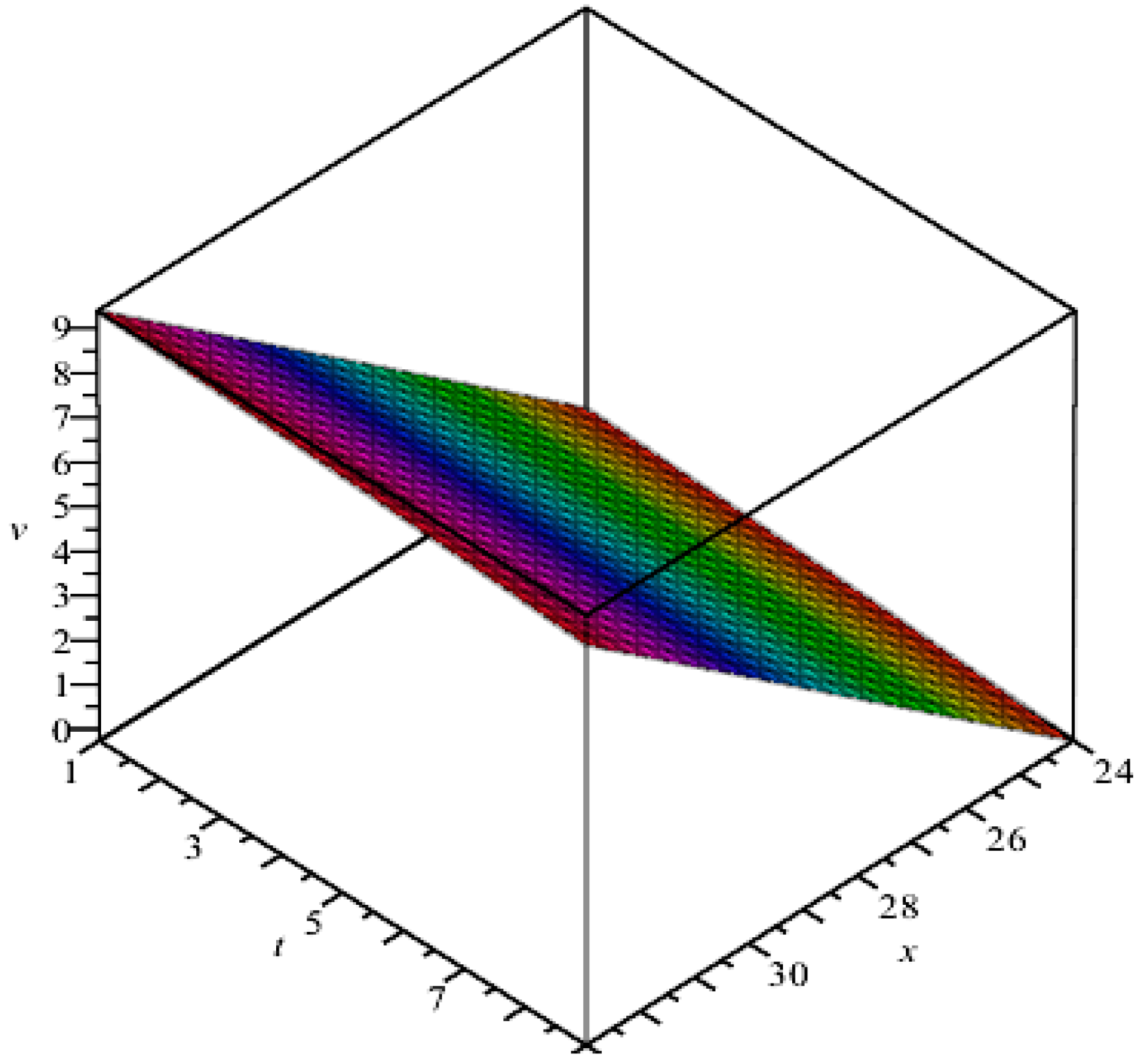
We present in this section Figure 1, Figure 2, Figure 3 and Figure 4 to discuss our obtained results in comparison with their associated exact forms.
Figure 1.
.
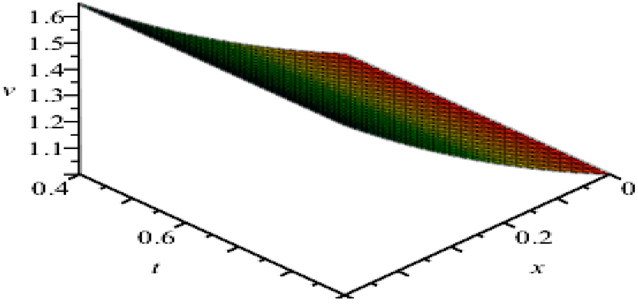
Figure 2.
.
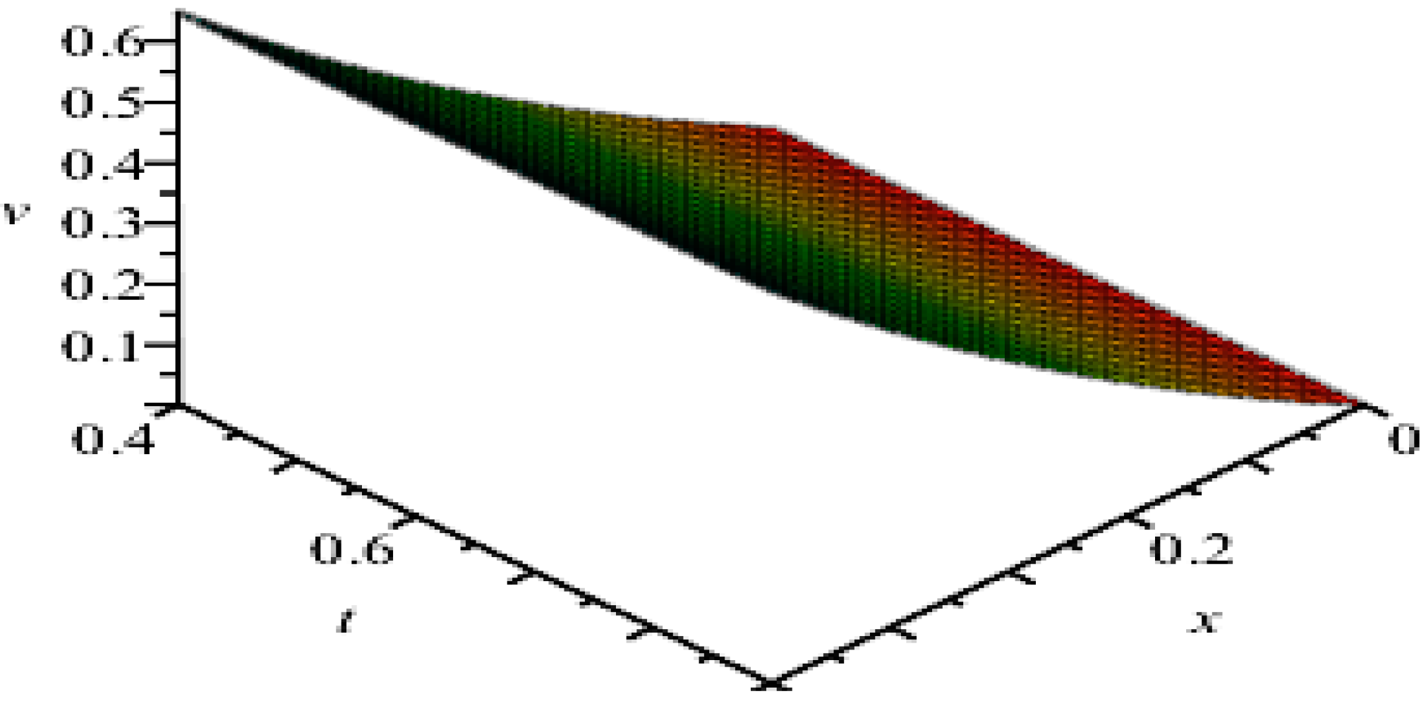
Figure 1 and Figure 2 are 3D plots of solutions to the problem in Example 1 at different values of for fixed .
Figure 3.
.
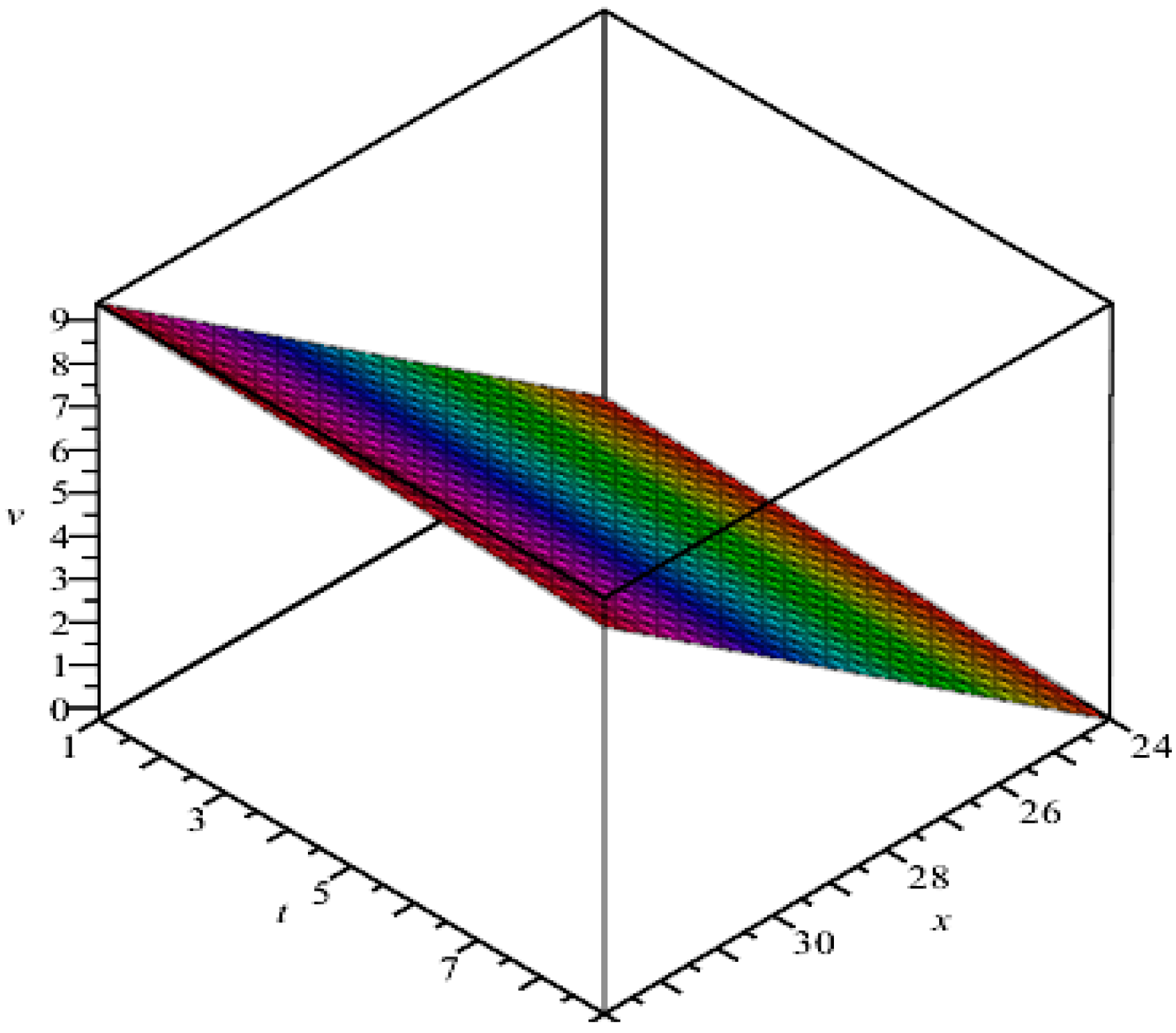
Figure 4.
.
5. Concluding Remarks
In this study, a proposed computational method known as Projected Differential Transformation Method (PDTM) has been successfully applied, for the first time, to the Black–Scholes Equation for European Option Valuation. We solved some illustrative and numerical examples to test the efficiency of the proposed method. The results obtained converge faster to their associated exact solutions, even with less computation, without linearization or perturbation; showing that the method can also be used easily for approximate solutions in a direct form; these easily computed results represent the analytical values of the associated European call options, the same algorithm can be followed for European put options.
Finally, we remarked that the PDTM is very efficient, reliable; and faster in application (even without giving up accuracy) when compared with the classical DTM [20], ADM [17], HAM and HPM [12]; though the results via these methods are in strong agreement. Hence, it is strongly recommended for both linear and nonlinear stochastic differential equations (SDEs) encountered in financial mathematics and other areas of applied sciences.
Acknowledgments
The authors are grateful to Covenant University for all forms of support not limited to finance, resources, good working environment, and spirituality. We thank the anonymous reviewers sincerely for their valuable time and constructive comments towards the improvement of the paper.
Author Contributions
All the authors: S.O.E., O.O.U., and E.A.O. carried out this work in collaboration with positive contribution. They all read and approved the final manuscript for publication.
Conflicts of Interest
The authors declare no conflict of interest.
References
- Black, F.; Scholes, M. The pricing of options and corporate liabilities. J. Political Econ. 1973, 81, 637–354. [Google Scholar] [CrossRef]
- Owoloko, E.A.; Okeke, M.C. Investigating the Imperfection of the B-S Model: A Case Study of an Emerging Stock Market. Br. J. Appl. Sci. Technol. 2014, 4, 4191–4200. [Google Scholar] [CrossRef]
- John, J.C.H. Options, Futures, and Other Derivatives, 9th ed.; Prentice Hall: Upper Saddle River, NJ, USA, 2014. [Google Scholar]
- Ugbebor, O.O.; Edeki, S.O. On Duality Principle in Exponentially Le’vy Market. J. Appl. Math. Bioinform. 2013, 3, 159–170. [Google Scholar]
- Yao, K. A no-arbitrage theorem for uncertain stock model. Fuzzy Optim. Decis. Mak. 2015, 14, 227–242. [Google Scholar] [CrossRef]
- Chen, X.W. American option pricing formula for uncertain financial market. Int. J. Oper. Res. 2011, 8, 32–37. [Google Scholar]
- Li, S.; Peng, J. A new stock model for option pricing in uncertain environment. Iran. J. Fuzzy Syst. 2014, 11, 27–41. [Google Scholar] [CrossRef]
- Jiao, D.Y.; Yao, K. An interest rate model in uncertain environment. Soft Comput. 2015, 19, 775–780. [Google Scholar] [CrossRef]
- Oksendel, B. Stochastic Differential Equation; Springer: Berlin/Heidelberg, Germany, 1991. [Google Scholar]
- Brzezniak, Z.; Zastawniak, T. Basic Stochastic Processes; Springer Verlag: Heidelberg, Germany, 1998. [Google Scholar]
- Zheng, Y. On Stochastic Differential Equation and Modified Black–Scholes Option Pricing Model. Available online: http://ssrn.com/abstract=1091823 (accessed on 9 October 2015).
- Smeureanu, I.; Fanache, D. A Linear Algorithm for Black–Scholes Economic Model. Rev. Inform. Econ. 2008, 1, 150–156. [Google Scholar]
- Cen, Z.; Le, A. A robust and accurate finite difference method for a generalized Black–Scholes equation. J. Comput. Appl. Math. 2011, 235, 3728–3733. [Google Scholar] [CrossRef]
- Mosneagu, A.M.; Dura, G. Numerical Approximation of Black–Scholes Equation. Ann. Alexandru Ioan Cuza Univ. Math. 2010, 56, 39–64. [Google Scholar]
- Uddin, M.K.S.; Ahmed, M.; Bhowmik, S.K. A Note on Numerical Solution of Linear Black–Scholes Model. GANIT J. Bangladesh Math. Soc. 2013, 33, 103–115. [Google Scholar] [CrossRef]
- Agliardi, R.; Popivanov, P.; Slovova, A. On Nonlinear Black–Scholes Equations. Nonl. Anal. Differ. Eq. 2013, 1, 75–81. [Google Scholar]
- Jodar, L.; Peris, P.S.; Cortes, J.C.; Sala, R. A new direct method for solving the Black–Scholes Equation. Appl. Math. Lett. 2005, 18, 29–32. [Google Scholar] [CrossRef]
- Qiu, Y.; Lorenz, J. A nonlinear Black–Scholes Equation. Int. J. Bus. Perform. Supply Chain Model. 2009, 1, 33–40. [Google Scholar] [CrossRef]
- Elbeleze, A.A.; Kilicman, A.; Taib, B.M. Homotopy Perturbation Method for Fractional Black–Scholes European Option Pricing Equations Using Sumudu Transform. Math. Probl. Eng. 2013, 2013. [Google Scholar] [CrossRef]
- Kumar, S.; Kumar, D.; Singh, J. Numerical Computation of Fractional Black–Scholes Equation arising in Financial Market. Egypt. J. Basic Appl. Sci. 2014, 1, 177–183. [Google Scholar] [CrossRef]
- Ahmad, J.; Shakeel, M.; UI Hassan, Q.M.; Mohyud-Din, S.T. Analytical Solution of Black–Scholes Model Using Fractional Variational Iteration Method. Int. J. Modern Math. Sci. 2013, 5, 133–142. [Google Scholar]
- Kumar, S.; Yildirin, A.; Khan, Y.; Jafari, H.; Sayevand, K.; Wei, L. Analytical Solution of Fractional Black–Scholes European Option Pricing Equations Using Laplace Transform. J. Fract. Calc. Appl. 2012, 2, 1–9. [Google Scholar]
- Bohner, M.; Sanchez, F.H.M.; Rodriguez, S. European Call Option Pricing Using the Adomian Decomposition Method. Adv. Dyn. Syst. Appl. 2014, 9, 75–85. [Google Scholar]
- Allahviranloo, T.; Behzadi, S.S. The use of iterative methods for solving Black–Scholes equations. Int. J. Ind. Math. 2013, 5, 1–11. [Google Scholar]
- Biazar, J.; Goldoust, F. The Adomian Decomposition Method for the Black–Scholes Equation. In Proceedings of the 3rd International Conference on Applied Mathematics and Pharmaceutical Sciences (ICAMP’2013), Singapore, Singapore, 29–30 April 2013; pp. 321–323.
- Edeki, S.O.; Adinya, I.; Ugbebor, O.O. The Effect of Stochastic Capital Reserve on Actuarial Risk Analysis via an Integro-differential equation. IAENG Int. J. Appl. Math. 2014, 44, 83–90. [Google Scholar]
- Demiray, S.T.; Bulut, H.; Belgacem, F.B.M. Sumudu Transform Method for Analytical Solutions of Fractional Type Ordinary Differential Equations. Math. Probl. Eng. 2014, 2014. [Google Scholar] [CrossRef]
- Kanth, A.S.V.R.; Aruna, K. Comparison of two Dimensional DTM and PDTM for solving Time-Dependent Emden-Fowler Type Equations. Int. J. Nonlinear Sci. 2012, 13, 228–239. [Google Scholar]
- Dogan, N.; Erturk, V.S.; Akin, O. Numerical Treatment of Singularly Perturbed Two-Point Boundary Value Problems by Using Differential Transformation Method. Discrete Dyn. Nat. Soc. 2012, 2012. [Google Scholar] [CrossRef]
- Chen, C.K.; Ho, S.H. Solving partial differential equations by two-dimensional differential transform method. Appl. Math. Comput. 1999, 106, 171–179. [Google Scholar] [CrossRef]
- Jang, M.J.; Chen, C.L.; Liu, Y.C. Two-dimensional differential transform for partial differential equations. Appl. Math. Comput. 2001, 121, 261–270. [Google Scholar] [CrossRef]
- Sen, A.K. An Application of the Adomian decomposition method to the transcient behavior of a model of biochemical reaction. J. Math. Anal. Appl. 1988, 131, 232–245. [Google Scholar] [CrossRef]
- Mousa, M.M.; Ragab, S.F. Application of the Homotopy Perturbation Method to Linear and Nonlinear Schrodinger Equations. Verlag Z. Naturforschung Tubingen 2008, 63, 140–144. [Google Scholar] [CrossRef]
- Jang, B. Solving linear and nonlinear initial value problems by the projected differential transform method. Comput. Phys. Commun. 2010, 181, 848–854. [Google Scholar] [CrossRef]
- Ahmed, S.A.; Elzaki, T.M. A Comparative Study of Sumudu Decomposition Method and Sumudu Projected Differential Transform Method. World Appl. Sci. J. 2014, 31, 1704–1709. [Google Scholar]
© 2015 by the authors; licensee MDPI, Basel, Switzerland. This article is an open access article distributed under the terms and conditions of the Creative Commons Attribution license (http://creativecommons.org/licenses/by/4.0/).