Thermodynamic Analysis of Closed Steady or Cyclic Systems

Abstract

Closed, steady or cyclic thermodynamic systems, which have temperature variations over their boundaries, can represent an extremely large range of plants, devices or natural objects, such as combined heating, cooling and power plants, computers and data centres, and planets. Energy transfer rates can occur across the boundary, which are characterized as heat or work. We focus on the finite time thermodynamics aspects, on energy-based performance parameters, on rational efficiency and on the environmental reference temperature. To do this, we examine the net work rate of a closed, steady or cyclic system bounded by thermal resistances linked to isothermal reservoirs in terms of the first and second laws of thermodynamics. Citing relevant references from the literature, we propose a methodology that can improve the thermodynamic analysis of an energy-transforming or an exergy-destroying plant. Through the reflections and analysis presented, we have found an explanation of the second law that clarifies the link between the Clausius integral of heat over temperature and the reference temperature of the Gouy–Stodola theorem. With this insight and approach, the specification of the environmental reference temperature in exergy analysis becomes more solid. We have explained the relationship between the Curzon Ahlborn heat engine and an irreversible Carnot heat engine. We have outlined the nature of subsystem rational efficiencies and have found Rant’s anergy to play an important role. We postulate that heat transfer through thermal resistance is the sole basis of irreversibility.

1. Introduction

Closed, steady or cyclic thermodynamic systems, which have temperature variations over their boundaries, can represent an extremely large range of plants, devices or natural objects, such as combined heating, cooling and power plants, thermoelectric devices, regenerative and non-regenerative braking systems, energy storage systems, computers and data centres and planets. We consider a system closed if no matter crosses its boundary. We consider a closed system steady if its energy and entropy remain constant and if the distribution of temperature over the entropy transfer rate through its surface (Section 2.7) is invariant with time; with this definition, we do not require further information about its state. We consider a closed system cyclic if it returns one or more times to a state with the same energy, entropy and surface temperature distribution over the entropy transfer rate.

The analysis of a closed, steady or cyclic, reversible or irreversible system linked by thermal resistances to a heat source and a heat sink has been well studied in the literature, e.g., Novikov [1], Curzon and Ahlborn [2], Angulo-Brown et al. [3], Chen [4], Amelkin et al. [5], Feidt [6], Açıkkalp and Yamık [7] and Hernández et al. [8]. We use the term ‘reversible system’ to mean a system within which all processes are thermodynamically reversible and the term ‘irreversible system’ to mean a system within which some processes are not thermodynamically reversible. Many papers are concerned with establishing upper bounds for the thermal efficiency of a heat engine at maximum power, but general performance characteristics have also been examined for heat engines, reverse heat engines and plants with more than one useful output rate, i.e., a positive net rate of work output and/or exergy output rates corresponding to heat transfer rates at various temperatures.

We look at first law performance parameters and second law rational efficiencies of such arrangements, including cases where there are more than two isothermal reservoirs. For the configuration where there is only one isothermal reservoir in addition to the environmental isothermal reservoir, we demonstrate the relationships between energy-based thermal efficiencies or coefficients of performance (COPs) and second law rational efficiencies. For completeness, we introduce a new heat engine COP, applicable where the heat sink (the exergy source in this case) is at a temperature below the ambient one. This engine COP is a practical alternative to defining the thermal efficiency as the ratio of the power output to a rate of heat input at environmental temperature (this rate of heat transfer has no exergetic or economic value). It can be seen that there is nice symmetry between the expressions for thermal efficiencies, COPs and rational efficiencies that we present. Between them, they describe the complete first law and second law performance characteristics of the composite system investigated, not just the optimal performance. The composite, irreversible system has four operational cases: the heat engine (HE1) where the heat source is above the ambient temperature, the heat engine (HE2) where the heat sink is below the ambient temperature, the heat pump (reverse heat engine, RHE1) and the refrigeration plant (RHE2). We also present the rational efficiency at maximum power, which we have not found in the literature, although it is implicit. This is the rational efficiency of the Curzon–Ahlborn engine operating at maximum power.

Exergy analysis is based on the concept of an idealized, all-enclosing, reference environment that has infinite heat capacity and thermal conductivity, is uniform and is in equilibrium at the environmental reference temperature, $T_0$. The actual surroundings of a real plant, such as a heat engine, a heat pump or a refrigerator, may differ significantly from the ideal. We apply the concepts of finite time thermodynamics to refine the concept of $T_0$, thereby making exergy analysis more consistent with reality.

1.1. Model

As an actual ‘environment’ may not be in thermal equilibrium: a real plant may interact with multiple thermal reservoirs, e.g., with the ground, with a large body of water, with the air, with the sun and with the sky, as well as available sources of exergy, such as a combustion region or a source of waste heat. Usually, also, there will be at least one intended exergy sink, which needs to be adequately defined and characterized: it could be a sink of mechanical shaft power, a sink of electrical power or, as a pertinent example, an isothermal reservoir attached to the system by a thermal resistance. It should be noted too that an intended exergy sink could be a source of heat transfer at a temperature that is lower than $T_0$.

Referring to Figure 1, we consider a closed reversible or irreversible system, A, that produces a net shaft work interaction rate while undergoing heat transfer interactions with n isothermal reservoirs, each linked to the boundary of System A by a constant thermal resistance. The thermal resistances would have SI units of K/W. We assume that the physical regions associated with the thermal resistances have negligible heat capacity. We assume that the arrows shown in Figure 1 indicate the positive directions for the associated heat transfer rates and the net work rate.

Figure 1. A closed reversible or irreversible system, A, bounded by constant thermal resistances linked to isothermal reservoirs.

Figure 1. A closed reversible or irreversible system, A, bounded by constant thermal resistances linked to isothermal reservoirs.

As a key constraint, we assume that System A undergoes no net change. For simplicity, we assume that it is closed, as otherwise we would have to include net transport of energy and entropy in our energy and entropy balances. It may be in a steady state, but if its state is unsteady, the net work interaction rate is the time-averaged value, and the heat transfer rates are time-averaged values at stated fixed temperatures. A virtual isothermal reservoir at the effective environmental temperature, $T_0$, is also shown. As it is virtual, it has a heat transfer interaction rate of zero with A. Whenever we have only a single, isothermal, environmental reservoir, we will label its temperature $T_0$, and it need not be virtual, as it is likely to provide or accept a finite rate of heat transfer, ${\dot{Q}}_0$. It is a fundamental assumption of exergy analysis that there is a reservoir that can either supply or accept heat transfer at this fixed temperature, without limit.

An isothermal reservoir does not have to be infinite, as long as it can accept or provide the required heat transfer rate. Engineers know how to make such a thing, e.g., by making use of a thermoelectric device. We can maintain a temperature on the boundary. We also assume that we can vary or set the various heat transfer rates, as required. For this discussion, the thermal reservoirs are held at constant temperatures, just as Carnot [9] described for the hot and cold bodies in his book of 1824.

In Figure 1, we also show a second system, B, that includes A and the thermal resistances. At the boundary of System B, heat transfer occurs at the temperatures of the external isothermal reservoirs.

If there are just two isothermal reservoirs, then the heat engine would operate with one heat source and one heat sink. If the thermal resistances are negligible and System A is reversible, we would have a reversible Carnot cycle operating directly between the two isothermal reservoirs.

If there are n isothermal reservoirs, all of the thermal resistances are negligible and System A is reversible, then there could be multiple Carnot cycles involved. In fact, when we plot a general “cycle” of a reversible closed system that undergoes no net change on a temperature versus entropy-transfer-rate diagram (Section 2.7), every cycle is a Carnot cycle. In the translated book “The Mechanical Theory of Heat” of 1879, Clausius [10] broke up reversible cycles, plotted on diagrams of pressure against volume, into thin strips, each of which corresponded to a Carnot cycle. He used the diagram on p. 89 to explain his famous equality for a reversible cycle $\int \mathrm{d}Q/T=0$ and cited his original paper of 1854, published in Poggendorffs Annalen. In an analogous way, we can model any reversible closed system, within which no net change is occurring as it interacts with multiple thermal reservoirs, with an assembly of contiguous, but adiabatically-separated Carnot cycle systems. Moreover, we can model any irreversible closed system, within which no net change is occurring as it interacts with multiple thermal reservoirs, as an assembly of contiguous, but adiabatically-separated Carnot cycle systems bounded by thermal resistances, each of which interacts only with two isothermal reservoirs and a work reservoir. A work reservoir is a system that can accept or provide a rate of shaft work. Indeed, we can go further and allow the “Carnot” cycle to be irreversible. Where we are interested in modelling a range of operating conditions or the performance of subsystems, a finite-time thermodynamics model incorporating an irreversible cycle is likely to be closer to reality than one where all of the irreversibility is modelled by the bounding thermal resistances only.

The entropy transfer rate associated with a rate of heat transfer $\dot{Q_i}$ through a boundary that is at absolute temperature $T_i$ is given by Equation (1).

$$\dot{S_i}=\frac{\dot{Q_i}}{T_i}$$

(1)

We find it very useful to plot temperature against the cumulative rate of entropy transfer, over the surface of the assembly of Carnot cycle systems or the assembly of irreversible systems that involve heat transfer at two temperatures only, which undergo no net change, and over time. We have that sort of arrangement in mind when we put forward these n isothermal reservoirs. The integer n could have any value up to infinity, and if it is infinity, then we could have smooth temperature glides (over part of the boundary of the surface or over intervals of time). Hence, we can have constant temperatures and/or temperature glides.

Amelkin et al. [5,11] have considered a multiple reservoir arrangement of the type shown in Figure 1, both for the case where System A is reversible and where it involves irreversibility. In optimizing the plant for the maximization of power output, they came to the conclusion that not all thermal reservoirs should be chosen. In the present paper, we are not concerned with performing such an optimization, but rather with characterizing the performance of the overall system as it exchanges energy by heat transfer at specified rates with specified isothermal reservoirs.

1.2. Aims

Our first aim in this paper is to examine the energy-based, or first law, performance parameters of System B, consisting of a closed reversible system linked by thermal resistances to n isothermal reservoirs. In engineering, we still use first law performance quantifiers: specifically, thermal efficiencies and coefficients of performance. Equation (2) defines the thermal efficiency of a heat engine. Equations (3) and (4) define the coefficients of performance of a heat pump and a refrigeration plant, respectively. These performance parameters are traditional and convenient, but not entirely logical. An efficiency must be greater than or equal to zero and less than unity. A coefficient of performance must be greater than or equal to zero, but need not be less than unity.

$$E_{\mathrm{th}\mathrm{eng}}=\frac{{\dot{W}}_{\mathrm{net}\mathrm{out}}}{{\dot{Q}}_{\mathrm{in}}}=\frac{\mathrm{Desired}\mathrm{energy}\mathrm{output}\mathrm{rate}}{\mathrm{Necessary}\mathrm{energy}\mathrm{input}\mathrm{rate}}$$

(2)

$${\mathrm{COP}}_{\mathrm{hp}}=\frac{{\dot{Q}}_{\mathrm{out}}}{{\dot{W}}_{\mathrm{net}\mathrm{in}}}=\mathrm{ditto}$$

(3)

$${\mathrm{COP}}_{\mathrm{ref}}=\frac{{\dot{Q}}_{\mathrm{in}}}{{\dot{W}}_{\mathrm{net}\mathrm{in}}}=\frac{\mathrm{Desired}\mathrm{energy}\mathrm{input}\mathrm{rate}}{\mathrm{Necessary}\mathrm{energy}\mathrm{input}\mathrm{rate}}$$

(4)

For example, the performance of an ideal heat pump, as characterized by the Carnot COP, could be five or it might be thirty five. This is the COP of a reversible Carnot cycle, operating in reverse as a reverse heat engine. In 1852, William Thomson [12], Lord Kelvin, wrote a paper, “On the economy of heating or cooling of buildings by means of currents of air”, in which he came up with the ratio of the required work input to the heat transfer that would be required for the direct heating of the air as $1/35$. We would now describe such performance, using the inverse of Kelvin’s fraction, by quoting a heat pump COP of 35. In Kelvin’s calculations, the air was to be heated from 50 °F to 80 °F, i.e., from 10.00 °C to 16.67 °C. Based on these temperatures, the Carnot heat pump COP would have been 18.0. However, Kelvin based his calculations on increasing the temperature of the air reversibly using a non-steady-flow, open, reversible system. Equivalently, calculating the integrated Carnot COP over the temperature glide of the air as it is heated at constant pressure in a steady flow system by a series of infinitesimal Carnot heat pumps, we obtain an overall heat pump COP for the reversible heat pump of 35.3. Current technology heat pumps for heating houses yield a COP of up about four. We are a long way from the ideal performance that Kelvin described accurately in 1852. The value of the COP quoted for a real system does not inherently indicate what the performance could be for an ideal system providing the same effect.

We also wanted to present the second law performance parameters: the rational efficiency values for System B, implemented as a heat engine, a heat pump or a refrigeration plant. We were interested, also, in the rational efficiency values of subsystems of the overall system. In addition, we wanted to explore the meaning of the environmental reference temperature.

2. Concept Development

We adopt a methodology that may help us to extract the structure of and appreciate the nature of the exergy flow paths associated with heat transfer, provide insight into ways of defining rational efficiency in exergy analysis and make the choice of environmental reference temperature somewhat more solid and method based, recognizing the significance of finite time in real thermodynamic processes that involve heat transfer. We start with the simplest case and develop the concepts progressively.

2.1. One Heat Source and One Heat Sink with Reversible Heat Transfer

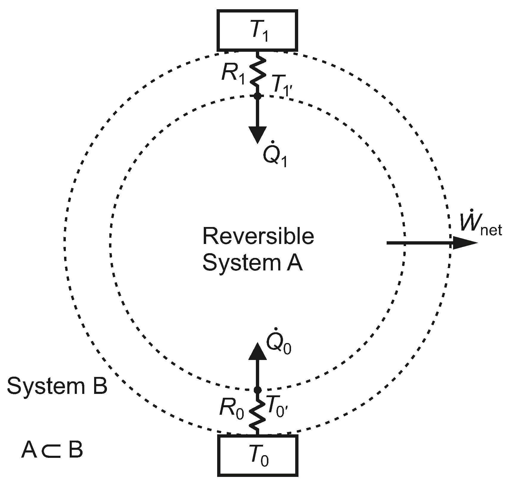
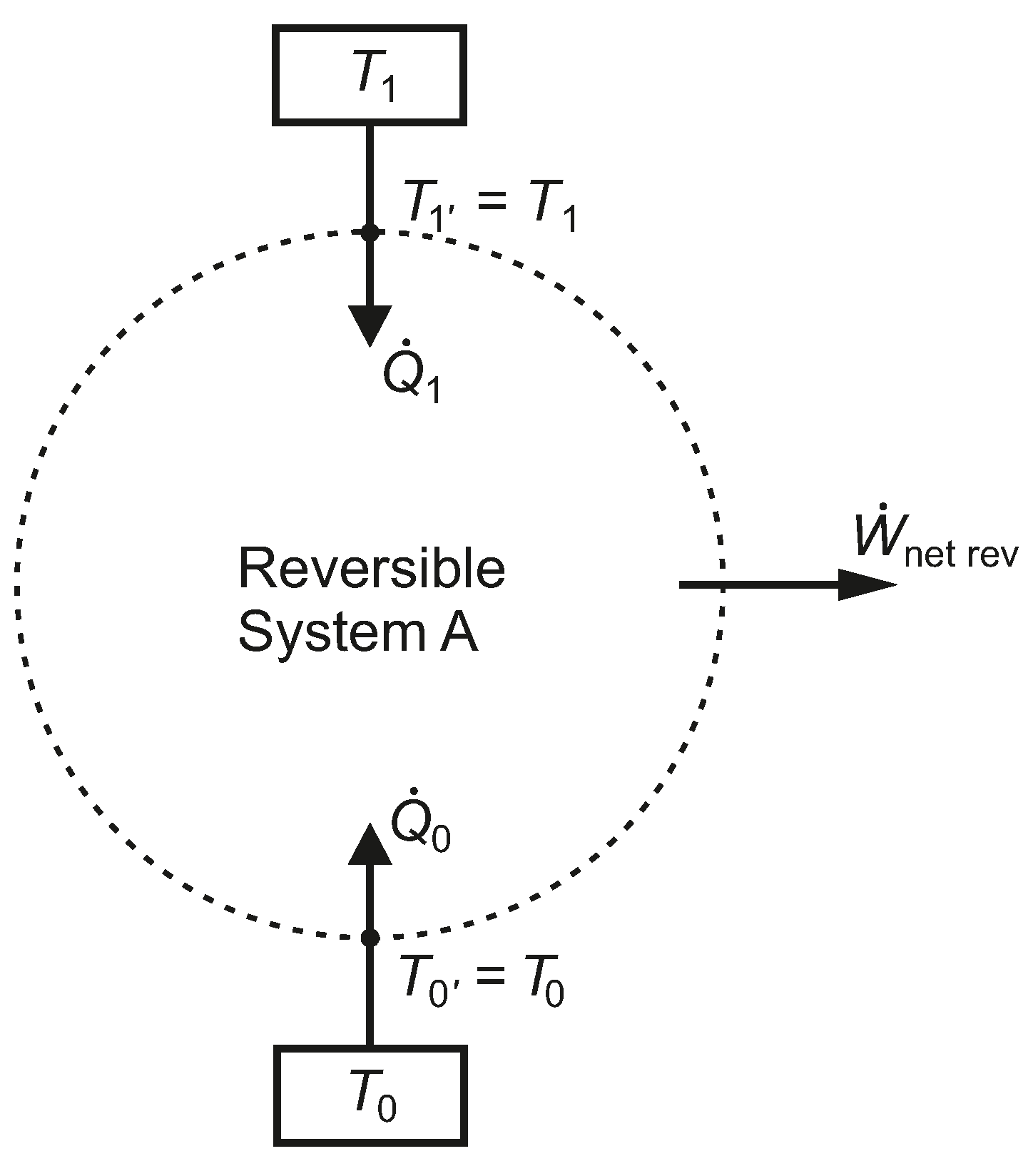
In Figure 2, a system, A, has a net work interaction while exchanging heat with just two isothermal reservoirs, at temperatures $T_1$ and $T_0$, where each thermal reservoir is linked to the boundary of the system, without any thermal resistance between them. For the moment, we assume the net work is an energy output and that $T_1>T_0$. We also assume that System A undergoes only reversible processes.

Figure 2. A closed reversible system, A, bounded by two isothermal reservoirs, without intermediate thermal resistances.

Figure 2. A closed reversible system, A, bounded by two isothermal reservoirs, without intermediate thermal resistances.

The thermal efficiency, $E_{\mathrm{th}\mathrm{rev}}$, is given by Equation (5), and the net rate of work output is given by Equation (6). This efficiency is known as the Carnot efficiency, $E_{\mathrm{Carnot}}$, as Sadi Carnot [9] first described the concept of an idealized cycle of a heat engine system, based on reversible processes and with only infinitesimal temperature differences causing the heat transfer interactions between the system and two isothermal reservoirs. Carnot also pointed out that this maximum efficiency, expressing the “motive power” of the heat transfer rates, was independent of the particular working substance, whether solid, liquid, vapour or two-phase. The Carnot efficiency would be applicable for any net rate of work output of a reversible steady-state or cyclic device, operating between the two isothermal reservoirs, for which the assumption of zero or infinitesimal connecting thermal resistances held.

$$E_{\mathrm{th}\mathrm{rev}}=\frac{{\dot{W}}_{\mathrm{net}\mathrm{rev}}}{{\dot{Q}}_1}=E_{\mathrm{Carnot}}=\left(\frac{T_1-T_0}{T_1}\right)=\left(1-\frac{T_0}{T_1}\right)$$

(5)

$${\dot{W}}_{\mathrm{net}\mathrm{rev}}={\dot{Q}}_1\left(1-\frac{T_0}{T_1}\right)$$

(6)

Now, we consider cases where the net work interaction is an energy input and where $T_1$ may be greater than or less than $T_0$. Carnot [9] (p.11) pointed out that the net work output of his idealized heat engine could be reversed, so that the energy taken from the source and that transferred to the sink could be returned, leaving no net effect on the heat engine system or its surroundings. The heat pump and refrigeration COPs of a reversible heat engine, operating in reverse, are given by Equations (7) and (8).

$${\mathrm{COP}}_{\mathrm{hp}\mathrm{rev}}=\frac{{\dot{Q}}_1}{{\dot{W}}_{\mathrm{net}\mathrm{rev}}}=\frac{1}{E_{\mathrm{Carnot}}}=\left(\frac{T_1}{T_1-T_0}\right)$$

(7)

$${\mathrm{COP}}_{\mathrm{refr}\mathrm{rev}}=-\frac{{\dot{Q}}_1}{{\dot{W}}_{\mathrm{net}\mathrm{rev}}}=-\frac{1}{E_{\mathrm{Carnot}}}=\left(\frac{T_1}{T_0-T_1}\right)$$

(8)

In Equation (7), ${\dot{Q}}_1$ and ${\dot{W}}_{\mathrm{net}\mathrm{rev}}$ are both negative, and the isothermal reservoir at temperature $T_1$ is the heat sink at a temperature above $T_0$. In Equation (8), ${\dot{W}}_{\mathrm{net}\mathrm{rev}}$ is negative, and the isothermal reservoir at temperature $T_1$ is the heat source, which is at a temperature below $T_0$.

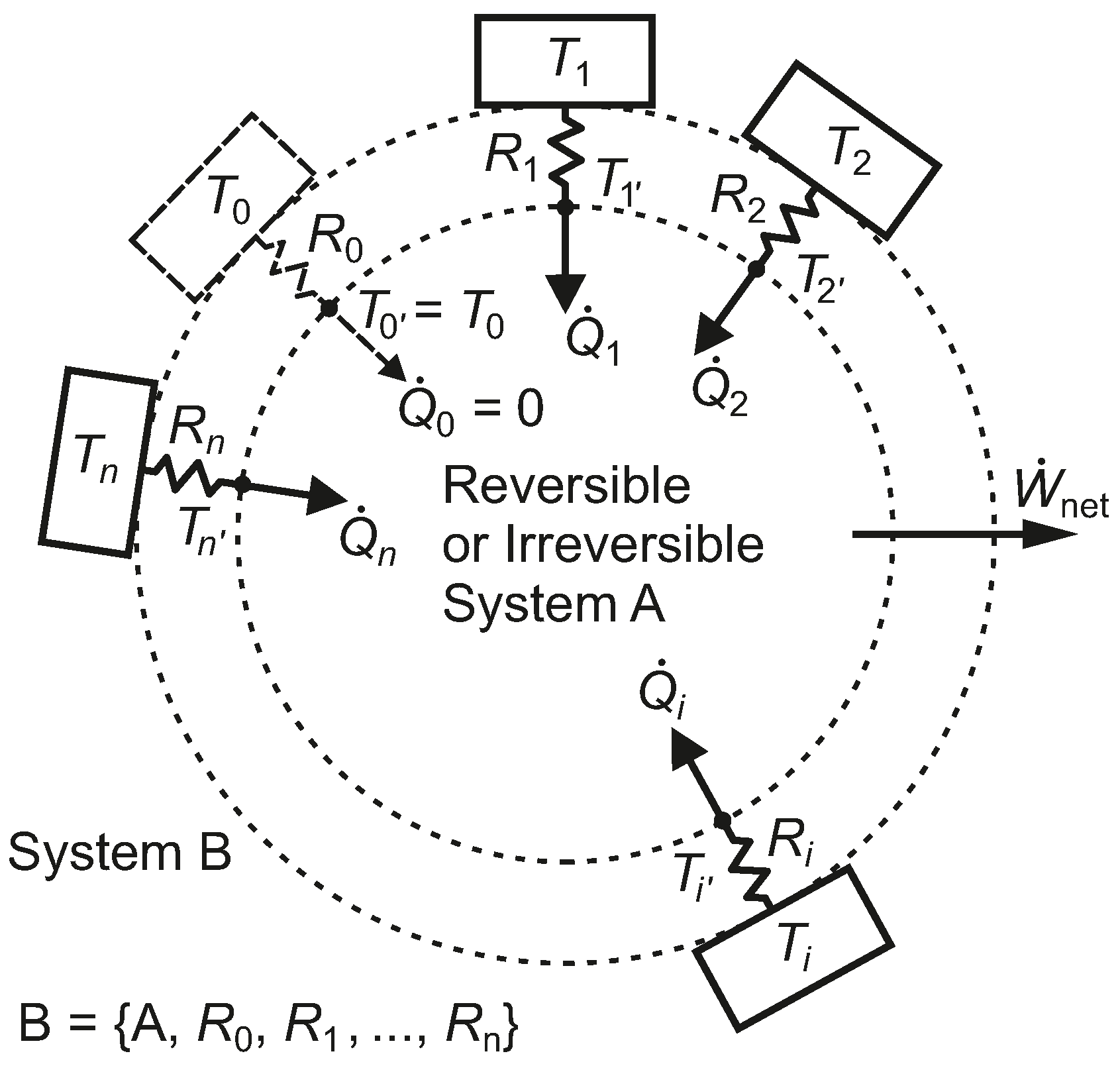
There remains a further case to be considered. Imagine we had an isothermal reservoir somewhere under the surface of the Earth at −100 ${}^{\circ }$C. Then, our heat engine could operate between ambient temperature, $T_0$, and that low-temperature reservoir, at $T_1$. This would be one of four different application cases that are possible. We could have:

• a heat engine (which we denote as HE1) accepting heat transfer from a high temperature heat source at $T_1$ and rejecting heat at $T_0$ (if irreversible, the entropy transfer rate out at $T_0$ is greater than the entropy transfer rate in at $T_1$),
• a heat engine (HE2) accepting heat transfer at $T_0$ and rejecting heat to a low temperature heat sink at $T_1$ (if irreversible, the entropy transfer rate out at $T_1$ is greater than the entropy transfer rate in at $T_0$),
• a heat pump (which we denote as a reverse heat engine, Type 1, RHE1) rejecting heat to a high temperature sink at $T_1$ and accepting heat transfer at $T_0$ (if irreversible, the entropy transfer rate out at $T_1$ is greater than the entropy transfer rate in at $T_0$) or,
• a refrigerator (RHE2) accepting heat transfer from a low temperature source at $T_1$ and rejecting heat at $T_0$ (if irreversible, the entropy transfer rate out at $T_0$ is greater than the entropy transfer rate in at $T_1$).

The Type 1 systems or devices (HE1 and RHE1) operate at temperatures that are mainly above ambient temperature, while Type 2 (HE2 and RHE2) operates mainly at temperatures below ambient temperature. In all four cases, entropy has to be balanced to respect the second law, which states that for a system that is undergoing no net change, the rate of entropy creation must be greater than or equal to zero and can only equal zero if there is no irreversibility occurring within the system. Where entropy is being created within the system, there must be a corresponding net rate of entropy rejection from the system. As a consequence, for a unique net rate of entropy transfer into the system (positive or negative) from the thermal energy reservoir at $T_1$ (this reservoir either provides or accepts a rate of exergy transfer) and a unique rate of entropy generation within the system, there must be a unique rate of heat transfer into or out of the environmental isothermal reservoir at $T_0$: the existence of the environmental isothermal reservoir allows this balancing heat transfer rate to occur. It could be called a rate of anergy transfer, using the term proposed by Rant [13]. It may be that progress in the field of exergy analysis and finite time thermodynamics has been held back by a lack of attention to anergy transfer.

Cases HE1 and HE2 are the heat engine cases where $T_1>T_0$ or $T_1<T_0$. There is a net rate of exergy input associated with heat transfer at $T_1$ and a net rate of exergy output as work. RHE1 and RHE2 are the reverse heat engine cases where $T_1>T_0$ or $T_1<T_0$. There is a net rate of exergy input as work and a net rate of exergy output associated with heat transfer at $T_1$.

For a reversible HE2, where $T_1<T_0$, the following expressions apply.

$$E_{\mathrm{th}\mathrm{rev}}{|}_{T_1<T_0}=E_{\mathrm{Carnot}}=\left(\frac{T_0-T_1}{T_0}\right)=\left(1-\frac{T_1}{T_0}\right)$$

(9)

$${\dot{W}}_{\mathrm{net}\mathrm{rev}}{|}_{T_1<T_0}={\dot{Q}}_0\left(1-\frac{T_1}{T_0}\right)$$

(10)

2.2. One Heat Source and One Heat Sink with Thermal Resistances

Assuming an HE1 heat engine ($T_1>T_0$), taking into account the temperature drops associated with heat transfer through resistances $R_1$ and $R_0$ in Figure 3 and letting $R_{\mathrm{tot}}=R_1+R_0$, the thermal efficiency is given by Equation (11) and the net power output by Equation (12).

$$E_{\mathrm{th}}{|}_{T_1>T_0}=1-\frac{T_0}{T_1-{\dot{Q}}_1{R}_{\mathrm{tot}}}$$

(11)

$${\dot{W}}_{\mathrm{net}}{|}_{T_1>T_0}={\dot{Q}}_1\left(1-\frac{T_0}{T_1-{\dot{Q}}_1{R}_{\mathrm{tot}}}\right)$$

(12)

Figure 3. A closed reversible system, A, bounded by two constant thermal resistances linked to isothermal reservoirs.

Figure 3. A closed reversible system, A, bounded by two constant thermal resistances linked to isothermal reservoirs.

Assuming an HE2 heat engine ($T_1<T_0$), the thermal efficiency is given by Equation (13) and the net power output by Equation (14). We note that the thermal efficiency is still defined as the net rate of work output divided by the rate of heat input and that, in this case, the rate of heat input is ${\dot{Q}}_0$.

$$E_{\mathrm{th}}{|}_{T_1<T_0}=\frac{{\dot{W}}_{\mathrm{net}}}{{\dot{Q}}_0}=1-\frac{T_1}{T_0-{\dot{Q}}_0{R}_{\mathrm{tot}}}$$

(13)

$${\dot{W}}_{\mathrm{net}}{|}_{T_1<T_0}={\dot{Q}}_0\left(1-\frac{T_1}{T_0-{\dot{Q}}_0{R}_{\mathrm{tot}}}\right)$$

(14)

The heat pump and refrigeration COPs are given by Equations (15) and (16).

$${\mathrm{COP}}_{\mathrm{hp}}=\frac{-{\dot{Q}}_1}{-{\dot{W}}_{\mathrm{net}}}=\frac{1}{E_{\mathrm{th}}}=\left(\frac{T_1-{\dot{Q}}_1{R}_{\mathrm{tot}}}{T_1-T_0-{\dot{Q}}_1{R}_{\mathrm{tot}}}\right)$$

(15)

$${\mathrm{COP}}_{\mathrm{refr}}=\frac{{\dot{Q}}_1}{-{\dot{W}}_{\mathrm{net}}}=-\frac{1}{E_{\mathrm{th}}}=\left(\frac{T_1-{\dot{Q}}_1{R}_{\mathrm{tot}}}{T_0-T_1+{\dot{Q}}_1{R}_{\mathrm{tot}}}\right)$$

(16)

At this point, we define one more first law performance parameter that we will refer to subsequently as part of our second law analysis of HE2 heat engines. We use the engine COP of Equation (17) for an HE2 to express the ratio of the net work output rate to the rate of heat rejection to the low temperature sink at $T_1$, where $T_1<T_0$. The work output rate is given by Equation (18).

$${\mathrm{COP}}_{\mathrm{eng}}{|}_{T_1<T_0}=-\frac{{\dot{W}}_{\mathrm{net}}}{{\dot{Q}}_1}=\left(\frac{T_0}{T_1-{\dot{Q}}_1{R}_{\mathrm{tot}}}-1\right)$$

(17)

$${\dot{W}}_{\mathrm{net}}{|}_{T_1<T_0}={\dot{Q}}_1\left(1-\frac{T_0}{T_1-{\dot{Q}}_1{R}_{\mathrm{tot}}}\right)$$

(18)

2.3. Heat Input Rate and Thermal Efficiency of a Heat Engine at Maximum Power

For an HE1 heat engine (where $T_1>T_0$) at maximum net power output, the rate of heat input is given by Equation (19) and the thermal efficiency by Equation (20).

$${\dot{Q}}_{1,\max \mathrm{power}}{|}_{T_1>T_0}=\frac{T_1-\sqrt{T_1}\sqrt{T_0}}{R_{\mathrm{tot}}}$$

(19)

$$E_{\mathrm{th},\max \mathrm{power}}{|}_{T_1>T_0}=\frac{{\dot{W}}_{\mathrm{net},\max \mathrm{power}}}{{\dot{Q}}_{1,\max \mathrm{power}}}=1-\frac{\sqrt{T_0}}{\sqrt{T_1}}$$

(20)

Similar expressions can be written for an HE2 heat engine: Equations (21) and (22). We also provide Equations (23) and (24), as we regard ${\dot{Q}}_1$ as the principal heat transfer rate.

$${\dot{Q}}_{0,\max \mathrm{power}}{|}_{T_1<T_0}=\frac{T_0-\sqrt{T_0}\sqrt{T_1}}{R_{\mathrm{tot}}}$$

(21)

$$E_{\mathrm{th},\max \mathrm{power}}{|}_{T_1<T_0}=\frac{{\dot{W}}_{\mathrm{net},\max \mathrm{power}}}{{\dot{Q}}_{0,\max \mathrm{power}}}=1-\frac{\sqrt{T_1}}{\sqrt{T_0}}$$

(22)

$${\dot{Q}}_{1,\max \mathrm{power}}{|}_{T_1<T_0}=\frac{T_1-\sqrt{T_0}\sqrt{T_1}}{R_{\mathrm{tot}}}$$

(23)

$${\mathrm{COP}}_{\mathrm{eng},\max \mathrm{power}}{|}_{T_1<T_0}=-\frac{{\dot{W}}_{\mathrm{net},\max \mathrm{power}}}{{\dot{Q}}_{1,\max \mathrm{power}}}=1-\frac{\sqrt{T_0}}{\sqrt{T_1}}$$

(24)

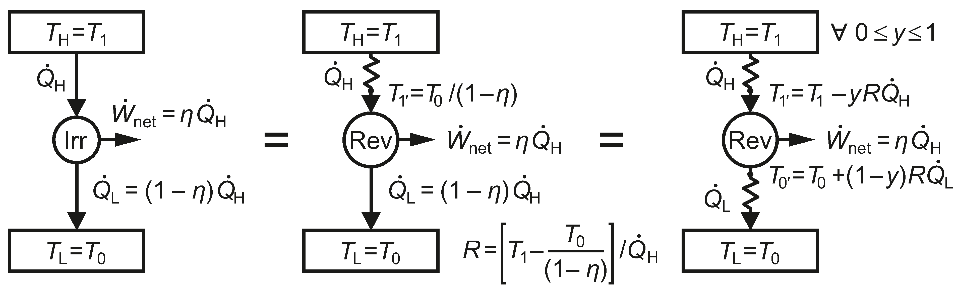
Vaudret et al. [14] have traced the history of Equation (20) to a 1929 book by Reitlinger and have included a scanned image of the relevant excerpt in their paper. Furthermore, an equation equivalent to Equation (20) for thermal efficiency was provided by Novikov [1], where $T_1$ was the temperature at which heat transfer evolved in a nuclear reactor and $T_0$ was the ambient temperature. As a simplification underlying this form of the equation, the working fluid cycle was assumed to be reversible. Novikov credited a number of other authors with developing this type of expression. Equation (20) was popularized by Curzon and Ahlborn [2], and their paper has been very widely cited.

Equations (11), (12) and (16) were included (the last in two end-of-chapter problems) for the first time in the seventh edition (2013) of the popular heat and mass transfer textbook by Incropera et al. [15], emphasizing a growing appreciation of the structural relationship between the temperature differences associated with heat transfer interactions and optimization of plant performance—the papers by Novikov [1] and Curzon and Ahlborn [2] were cited. As an example, McGovern and Harte [16,17] included internal thermal resistances in exergy analyses of the operation of refrigeration compressors.

We note that System B in Figure 3, which undergoes irreversible processes, has the same thermal efficiency as System A, which undergoes only reversible processes. The fact that both systems have the same thermal efficiency emphasizes the weakness of a first-law-only parameter, such as $E_{\mathrm{th}}$, for characterizing the performance of the heat engine. Systems B and A also share the same heat pump or refrigeration COPs.

2.4. Exergy Analysis Principles to Be Applied

The equality of Clausius [10], Equation (25), applies to the reversible system, A, of Figure 3, while his inequality, Equation (26), applies to the irreversible system, B, that includes the thermal resistances.

$$\sum _{i=0}^1\frac{{\dot{Q}}_i}{T_i^{\prime }}=0$$

(25)

$$\sum _{i=0}^1\frac{{\dot{Q}}_i}{T_i}<0$$

(26)

Here, we write Clausius’ expressions on a time rate basis for a closed, steady or cyclic system. If the system is steady, the summation is performed over the surface, requiring knowledge of the distribution of the heat flux and temperature. If the system is cyclic, the summation is performed over the surface and over time, requiring knowledge of the distribution of heat flux and temperature over the surface and over time. These expressions represent the second law of thermodynamics, while Equation (27) represents the first law.

$$\sum _{i=0}^1\dot{Q_i}={\dot{W}}_{\mathrm{net}}$$

(27)

Equations (25), (26) and (27) give rise to the Gouy–Stodola theorem, Equation (28), a derivation of which is available in Bejan [18] (Ch. 2). In this equation, ${\dot{W}}_{\mathrm{lost},0}$ is the rate at which available work (also known as exergy) is destroyed, e.g., in System B in Figure 3, and ${\dot{S}}_{\mathrm{gen}}$ is the rate of entropy generation within the system. In including a zero in the subscript label of ${\dot{W}}_{\mathrm{lost},0}$, Bejan explained and emphasized that the expressed rate at which available work is destroyed is with reference to an associated energy transfer rate (also known as an anergy transfer rate in this context) occurring at the specified environmental reference temperature $T_0$.

As Bejan [18] (Ch. 2) explained, it is common to draw the boundary of an overall system being analysed in entropy generation minimization analysis (or in exergy analysis) conventionally, in such a way that the ultimate ‘balancing’ transfer of energy to or from the environment occurs at $T_0$. The Gouy–Stodola theorem applies for just this case, but is not applicable for systems, or particularly subsystems, subject to constraints, such as being adiabatically separated from the environment, or bounded by a surface over which different or varying temperatures exist, or being bounded by an external surface of the overall system over which different environmental temperatures exist. Any entropy creation within a closed, steady or cyclic system undergoing no net change will require entropy transfer out of the system somewhere on the boundary, at some temperature, or over some ranges of temperature. If the system is steady, the rate of entropy rejection must be contemporaneous with the rate of entropy creation. In addition to writing Equation (28) with a zero in the identifying subscript of the lost work term, Bejan also provided an equation, equivalent to Equation (29), that allowed the lost work to be expressed relative to an associated reference temperature, $T_j$, on a system or subsystem boundary where balancing heat transfer or balancing entropy transport or transfer occur to satisfy the inequality of Clausius. This could be for cases where we are interested in the performance of a subsystem in the context of its own local constraints. We borrow this concept in relation to the exergy transfer rate associated with a rate of heat transfer, which we refer to an appropriate boundary temperature, Equation (30) and Figure 4.

$${\dot{W}}_{\mathrm{lost},0}=T_0{\dot{S}}_{\mathrm{gen}}$$

(28)

$${\dot{W}}_{\mathrm{lost},j}=\frac{T_j}{T_0}{\dot{W}}_{\mathrm{lost},0}$$

(29)

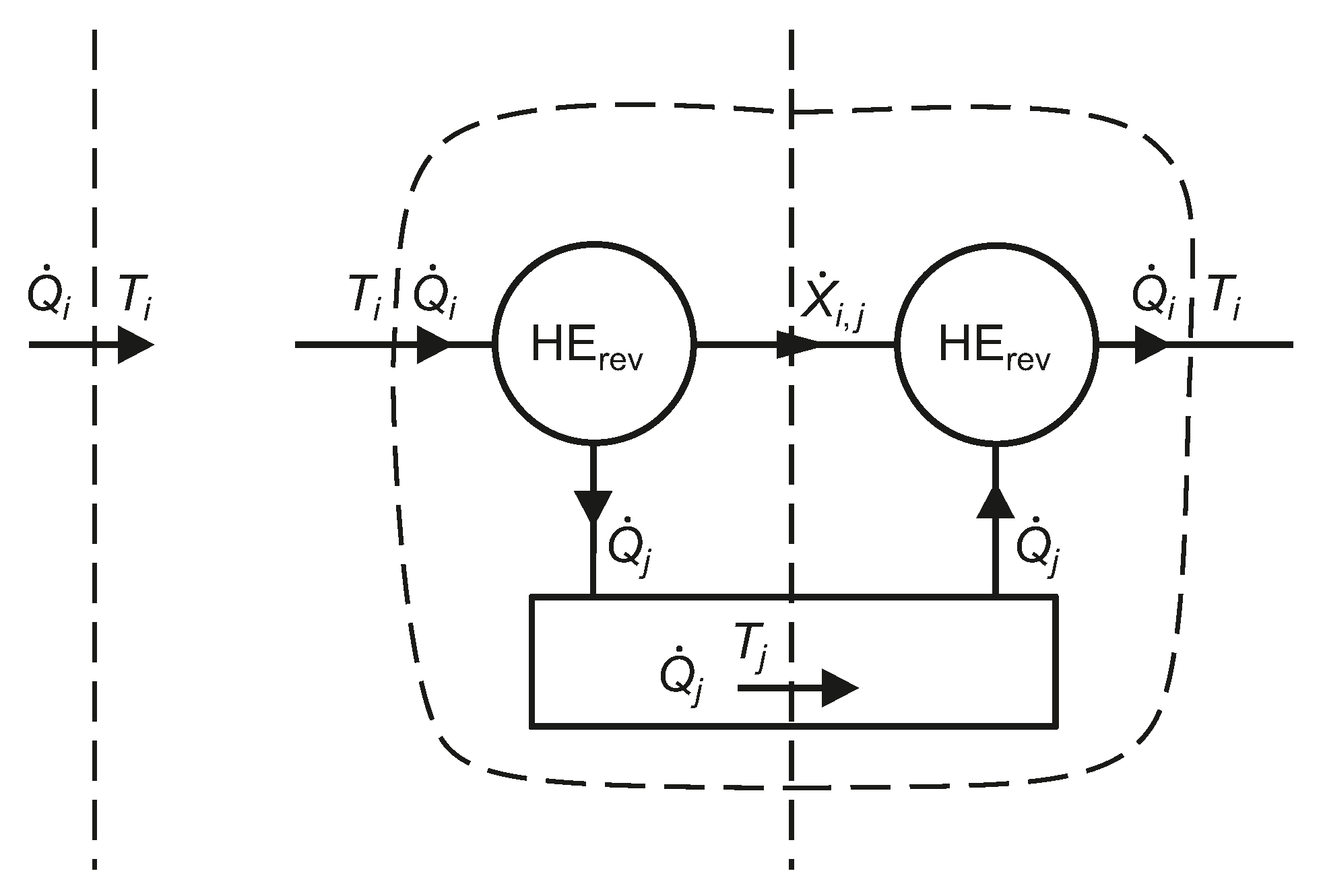
From the Carnot efficiency of a reversible engine operating between isothermal reservoirs at $T_i$ and $T_j$, the reversible shaft work associated with a heat transfer rate ${\dot{Q}}_i$ at $T_i$ is given by Equation (30), as explained schematically in Figure 4. The algebraic sign of the exergy transfer rate is automatically taken into account [19], but care is needed in its interpretation. The exergy transfer rate $\dot{X}$ will have the same sign as $\dot{Q}$ if $T>T_0$, but will have the opposite sign if $T<T_0$. In a vapour compression refrigeration plant, the energy transfer rate to the refrigerant in the evaporator is an input to the refrigeration system, but the corresponding exergy transfer rate is a negative input, which means that the exergy output rate is positive. Thus, Equation (30) gives the exergy transfer rate, ${\dot{X}}_{i,j}$, associated with an actual heat transfer rate in the context of the temperature $T_j$ of an isothermal reservoir at which any required heat and entropy transfer to satisfy the inequality of Clausius can occur.

$${\dot{X}}_{i,j}={\dot{Q}}_i\left(1-\frac{T_j}{T_i}\right)={\dot{Q}}_i-{\dot{A}}_{i,j}$$

(30)

Figure 4. The exergy transfer rate, ${\dot{X}}_{i,j}$, corresponding to a heat transfer rate ${\dot{Q}}_i$ at $T_i$, relative to an isothermal reservoir at temperature $T_j$ (virtual reversible heat engines, HE${}_{\mathrm{rev}}$, are employed).

Figure 4. The exergy transfer rate, ${\dot{X}}_{i,j}$, corresponding to a heat transfer rate ${\dot{Q}}_i$ at $T_i$, relative to an isothermal reservoir at temperature $T_j$ (virtual reversible heat engines, HE${}_{\mathrm{rev}}$, are employed).

The rate of anergy transfer, ${\dot{A}}_{i,j}$, associated with a rate of heat transfer at temperature $T_i$ is given by Equation (31). We note that the rate of anergy transfer is directly proportional to the reference temperature $T_j$ (which is usually the same as $T_0$) and indirectly proportional to the temperature at which the heat transfer occurs. It follows from Equation (31) that the rate of anergy transfer associated with a rate of heat transfer is always in the same direction as the heat transfer. We also note that the anergy rate of a rate of heat transfer at a given temperature equals the corresponding entropy transfer rate multiplied by the reference temperature for exergy and anergy $T_j$, which we call $T_0$ if it applies for the entire composite system under consideration.

$${\dot{A}}_{i,j}={\dot{Q}}_i\frac{T_j}{T_i}={\dot{S}}_i{T}_j={\dot{S}}_i{T}_k\frac{T_j}{T_k}={\dot{A}}_{i,k}\frac{T_j}{T_k}$$

(31)

For our definition of rational efficiency, η, we use the ratio, for a specified system, of the sum of the net exergy outputs to all exergy sinks, divided by the sum of the net exergy inputs from all exergy sources; Equation (32). To be rigorous, we need to make the following stipulations. There can only be one or more sources or one or more sinks, not both, associated with the net work rate. Likewise, for any temperature or infinitesimal temperature range where heat transfer occurs over the boundary, there can only be one or more sources or one or more sinks, not both, for the associated exergy transfer rate. This definition is entirely boundary-based. If a net exergy output rate will ultimately be destroyed and is therefore not useful, we have the choice of extending the boundary into the reference environment to include that rate of exergy destruction, thereby eliminating it from the numerator of the rational efficiency.

$$\eta =\frac{\sum {\dot{X}}_{\mathrm{net},\mathrm{out}}}{\sum {\dot{X}}_{\mathrm{net},\mathrm{in}}}$$

(32)

In a seminal paper in 1986, Valero, Lozano and Muñoz [20] introduced the concept of exergetic cost, defined as the amount of exergy per unit time required to produce a physical flow, and proposed a set of propositions relating to it as part of a theory of exergy saving. The concepts introduced amounted to a new way of looking at overall systems in terms of the laws of thermodynamics and the principles of economics. For costing and rational efficiency evaluation purposes, their proposition 2P, “…all the products of a generic equipment have the same unit exergetic cost” is key to addressing furcations (or forks) in the flow of exergy through an overall system or plant. Lozano and Valero published a comprehensive paper on the theory of exergetic cost in 1993 [21]. In this publication, the corresponding proposition, P4b, had the wording “…if a unit has a product composed of several flows, then the same unit exergetic cost will be assigned to all of them”.

We believe exergetic costing approaches, and exergonomic approaches built on them will be more widely used as understanding of the nature of exergy flow through systems deepens. The reference temperature is of central importance, as the numerical outcomes are dependent on it. McGovern [22] focused on the structural issue of exergy recycles.

Now we point out the structural difference between a conventional mechanical efficiency of a power transmission system, such as a gearbox, and a rational efficiency according to Equation (32). The mechanical efficiency (shaft power output over input) could be 95%. The rational efficiency would typically be zero (where the analysis boundary extends into the environment). However, in principle the rational efficiency of an improved version could be higher than even the mechanical efficiency. If the materials could withstand it, we could cause the heat rejection rate (energetically equivalent to 5% of the input shaft power) to occur at a very high temperature relative to the temperature of the surroundings, $T_0$, and the net rate of exergy output could come arbitrarily close to the net input of mechanical power (input minus output shaft power).

2.5. Exergy Analysis of a Reversible System Linked without Thermal Resistances to Its Heat Source and Sink

We now apply exergy analysis to the reversible heat engine, A, described in Section 2.1 and Figure 2. We take $T_0$ to be the temperature of the environment. The net rate of work ${\dot{W}}_{\mathrm{net}\mathrm{rev}}$ is equivalent to a rate of shaft work, so it is also a rate of exergy transfer. If $T_1=T_0$, ${\dot{W}}_{\mathrm{net}\mathrm{rev}}$ can only be zero, and all rates of exergy output are zero, so the rational efficiency is undefined and irrelevant. In all other cases, the rational efficiency is unity.

If $T_1>T_0$ and ${\dot{W}}_{\mathrm{net}\mathrm{rev}}$ is positive, System A is a reversible heat engine (HE1) producing a net work output rate, ${\dot{X}}_{\mathrm{out},\mathrm{work}}$, according to Equation (6). We apply Equation (30) with $T_j=T_0$ to find the rates of exergy transfer associated with ${\dot{Q}}_0$ and with ${\dot{Q}}_1$, i.e., ${\dot{X}}_0=0$ and ${\dot{X}}_1={\dot{Q}}_1\left(1-T_0/T_1\right)$. Hence, the rational efficiency is given by:

$${\eta }_{\mathrm{eng}\mathrm{rev}}=\frac{{\dot{W}}_{\mathrm{net}\mathrm{rev}}}{{\dot{X}}_1}=\frac{{\dot{X}}_1+{\dot{X}}_0}{{\dot{X}}_1}=\frac{{\dot{Q}}_1\left(1-T_0/T_1\right)}{{\dot{Q}}_1\left(1-T_0/T_1\right)}=1$$

(33)

Similarly, if $T_1<T_0$ and ${\dot{W}}_{\mathrm{net}}$ is positive, System A is a reversible heat engine (HE2) producing a net work output rate. The rates of exergy transfer associated with ${\dot{Q}}_0$ and with ${\dot{Q}}_1$ are, once again, ${\dot{X}}_0=0$ and ${\dot{X}}_1={\dot{Q}}_1\left(1-T_0/T_1\right)$. We note that in this case, the exergy input rate is associated with the energy output rate $-{\dot{Q}}_1$. Hence, the rational efficiency is once again given as unity by Equation (33).

If $T_1>T_0$ and ${\dot{W}}_{\mathrm{net}\mathrm{rev}}$ is negative, System A is a reversible heat pump (RHE1) providing heat transfer to the isothermal reservoir at $T_1$. The rational efficiency is given by:

$${\eta }_{\mathrm{hp}\mathrm{rev}}=\frac{-{\dot{X}}_1}{-{\dot{W}}_{\mathrm{net}\mathrm{rev}}}=\frac{1}{{\eta }_{\mathrm{eng}\mathrm{rev}}}=1$$

(34)

If $T_1<T_0$ and ${\dot{W}}_{\mathrm{net}}$ is negative, System A is a reversible refrigerator (RHE2) accepting heat transfer from the isothermal reservoir at $T_1$ (an exergy output rate). The rational efficiency is given by:

$${\eta }_{\mathrm{refr}\mathrm{rev}}=\frac{-{\dot{X}}_1}{-{\dot{W}}_{\mathrm{net}\mathrm{rev}}}=\frac{1}{{\eta }_{\mathrm{eng}\mathrm{rev}}}=1$$

(35)

2.6. Exergy Analysis of a Reversible System Linked to Its Heat Source and Sink by Thermal Resistances

We now apply exergy analysis to Heat Engine B described in Section 2.2 and Figure 3. If $T_1=T_0$, ${\dot{W}}_{\mathrm{net}}$ can only be negative (i.e., an exergy input rate) or zero. The rates of exergy output can only be zero, so the rational efficiency is zero when ${\dot{W}}_{\mathrm{net}}$ is negative.

Using Equations (2), (13), (15), (16), (17) and (30), we obtain the following expressions for the rational efficiency where System B functions as a heat engine (denoted “eng”) or a heat engine operating in reverse (denoted “reng”, for “reverse engine”).

$${\eta }_{\mathrm{eng}}{|}_{T_1>T_0}=\frac{{\dot{W}}_{\mathrm{net}}}{{\dot{X}}_1}=\frac{T_1^2-({\dot{Q}}_1{R}_{\mathrm{tot}}+T_0)T_1}{(T_1-T_0)(T_1-{\dot{Q}}_1{R}_{\mathrm{tot}})}$$

(36)

$${\eta }_{\mathrm{eng}}{|}_{T_1<T_0}=\frac{{\dot{W}}_{\mathrm{net}}}{{\dot{X}}_1}=\frac{T_1^2-({\dot{Q}}_1{R}_{\mathrm{tot}}+T_0)T_1}{(T_1-T_0)(T_1-{\dot{Q}}_1{R}_{\mathrm{tot}})}$$

(37)

$${\eta }_{\mathrm{hp}}={\eta }_{\mathrm{reng}}{|}_{T_1>T_0}=\frac{-{\dot{X}}_1}{-{\dot{W}}_{\mathrm{net}}}=\frac{1}{{\eta }_{\mathrm{eng}}}=\frac{(T_1-T_0)(T_1-{\dot{Q}}_1{R}_{\mathrm{tot}})}{T_1^2-({\dot{Q}}_1{R}_{\mathrm{tot}}+T_0)T_1}$$

(38)

$${\eta }_{\mathrm{refr}}={\eta }_{\mathrm{reng}}{|}_{T_1<T_0}=\frac{-{\dot{X}}_1}{-{\dot{W}}_{\mathrm{net}}}=\frac{1}{{\eta }_{\mathrm{eng}}}=\frac{(T_1-T_0)(T_1-{\dot{Q}}_1{R}_{\mathrm{tot}})}{T_1^2-({\dot{Q}}_1{R}_{\mathrm{tot}}+T_0)T_1}$$

(39)

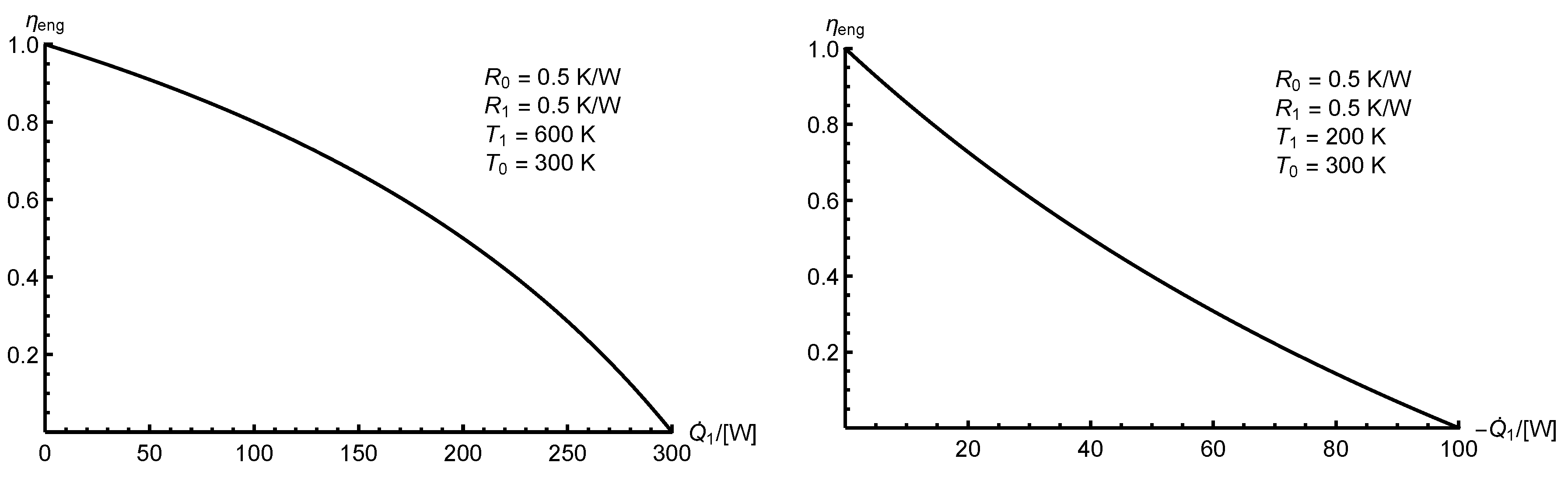
In Figure 5 and Figure 6 we provide sample rational efficiency plots versus the principal heat transfer rates, ${\dot{Q}}_1$, for heat engines (HE1 and HE2), a heat pump (RHE1) and a refrigeration plant (RHE2), each corresponding to the overall system, B, in Figure 3.

For a heat engine ($T_1>T_0$ or $T_1<T_0$) at maximum net power output, the rational efficiency is given by Equation (40).

$${\eta }_{\mathrm{eng},\max \mathrm{power}}=\frac{{\dot{W}}_{\mathrm{net}}}{{\dot{X}}_1}=\frac{1}{1+\sqrt{\frac{T_1}{T_0}}}$$

(40)

Figure 5. Rational efficiency versus the principal heat transfer rate, ${\dot{Q}}_1$, for heat engines ($T_1>T_0$ and $T_1<T_0$).

Figure 5. Rational efficiency versus the principal heat transfer rate, ${\dot{Q}}_1$, for heat engines ($T_1>T_0$ and $T_1<T_0$).

Figure 6. Rational efficiency versus the principal heat transfer rate, ${\dot{Q}}_1$, for reverse heat engines ($T_1>T_0$ and $T_1<T_0$).

Figure 6. Rational efficiency versus the principal heat transfer rate, ${\dot{Q}}_1$, for reverse heat engines ($T_1>T_0$ and $T_1<T_0$).

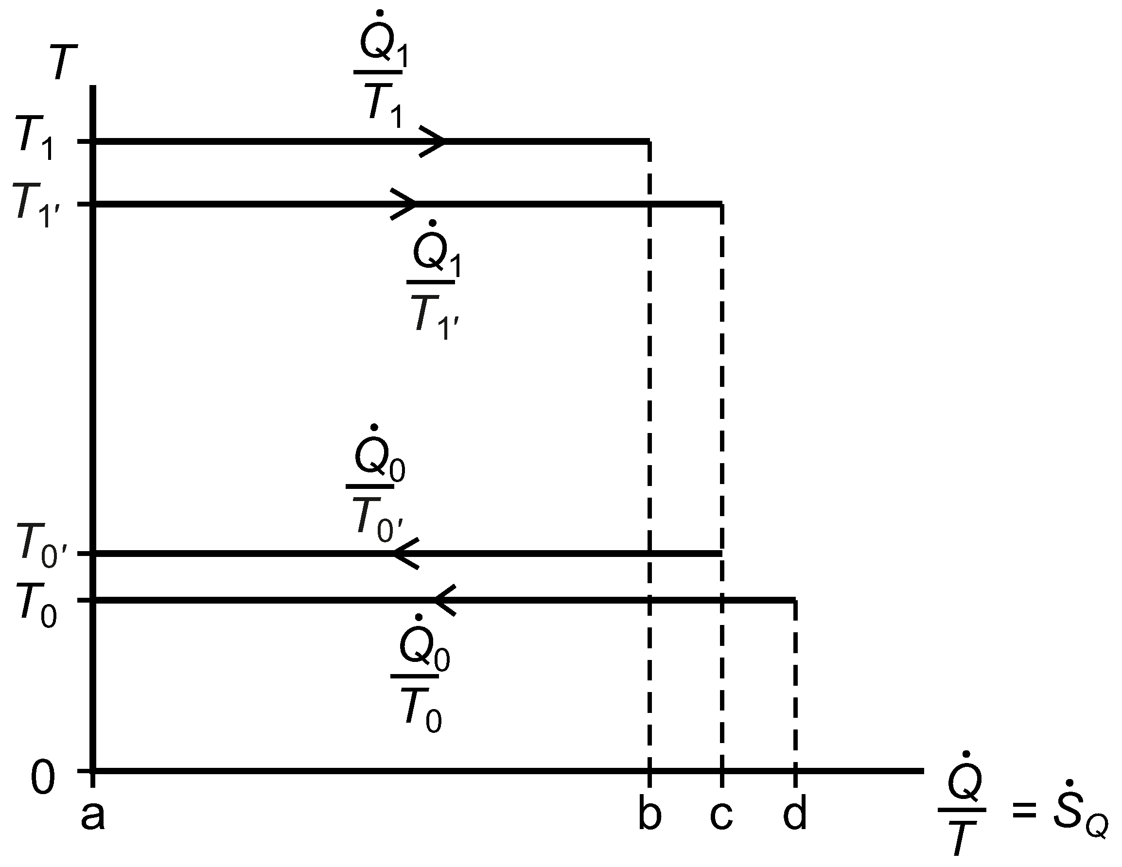
2.7. The Temperature versus Entropy Transfer Rate Diagram

We now consider the exergy analysis of the systems represented in Figure 3 with reference to a diagram of temperature versus entropy transfer rate for whichever system or subsystem we wish to focus on; Figure 7. Clausius’ cyclic integral, Equation (41), is applied over surface area and time to give the rate of entropy generation within any closed system or subsystem that undergoes no net change, and the Gouy–Stodola theorem, Equation (28), allows us to calculate the rate of lost work.

$$-\sum _i\frac{{\dot{Q}}_i}{T_i}={\dot{S}}_{\mathrm{gen}}$$

(41)

Figure 7. A diagram of temperature versus entropy transfer rates for a reversible heat engine linked by thermal resistances to two isothermal reservoirs, one of which is at the environmental temperature, $T_0$.

Figure 7. A diagram of temperature versus entropy transfer rates for a reversible heat engine linked by thermal resistances to two isothermal reservoirs, one of which is at the environmental temperature, $T_0$.

For System B, with respect to the environmental isothermal reservoir at $T_0$, the lost work rate is given by Equation (42) and the rate of exergy input is given by Equation (43).

$${\dot{W}}_{\mathrm{lost}\mathrm{B}}=T_0{\dot{S}}_{\mathrm{gen}\mathrm{B}}=-T_0\sum _{i=0}^1\frac{{\dot{Q}}_i}{T_i}=-T_0\left({\dot{S}}_{\mathrm{ab}}-{\dot{S}}_{\mathrm{ad}}\right)$$

(42)

$${\dot{X}}_{\mathrm{in}\mathrm{B}}={\dot{Q}}_1\left(1-\frac{T_0}{T_1}\right)={\dot{S}}_{\mathrm{ab}}\left(T_1-T_0\right)$$

(43)

The rational efficiency of System B with respect to $T_0$ is given by Equation (44). The quantities in this expression correspond to positive and negative rectangular areas in Figure 7.

$$\begin{array}{cc}\hfill {\eta }_{\mathrm{B},0}& =\frac{{\dot{X}}_{\mathrm{in}\mathrm{B}}-{\dot{W}}_{\mathrm{lost}\mathrm{B}}}{{\dot{X}}_{\mathrm{in}\mathrm{B}}}=\frac{{\dot{S}}_{\mathrm{ab}}\left(T_1-T_0\right)+T_0({\dot{S}}_{\mathrm{ab}}-{\dot{S}}_{\mathrm{ad}})}{{\dot{S}}_{\mathrm{ab}}\left(T_1-T_0\right)}\hfill \\ & =\frac{{\dot{S}}_{\mathrm{ab}}\left(T_1-T_0\right)-T_0{\dot{S}}_{\mathrm{bd}}}{{\dot{S}}_{\mathrm{ab}}\left(T_1-T_0\right)}=\frac{T_1(T_{1^{\prime }}-T_{0^{\prime }})}{T_{1^{\prime }}(T_1-T_0)}=\frac{T_1^2-({\dot{Q}}_1{R}_{\mathrm{tot}}+T_0)T_1}{(T_1-T_0)(T_1-{\dot{Q}}_1{R}_{\mathrm{tot}})}\hfill \end{array}$$

(44)

We also provide rational efficiency expressions for Systems A, $R_1$ and $R_0$ with respect to their entropy balancing reference temperatures $T_{0^{\prime }}$, $T_{1^{\prime }}$ and $T_0$, respectively; Equations (45)–(47).

$${\eta }_{\mathrm{A},0^{{}^{\prime }}}=\frac{{\dot{X}}_{\mathrm{in}\mathrm{A},0^{{}^{\prime }}}-{\dot{W}}_{\mathrm{lost}\mathrm{A},0^{{}^{\prime }}}}{{\dot{X}}_{\mathrm{in}\mathrm{A},0^{{}^{\prime }}}}=\frac{{\dot{S}}_{\mathrm{ac}}(T_{1^{\prime }}-T_{0^{\prime }})+T_{0^{\prime }}({\dot{S}}_{\mathrm{ac}}-{\dot{S}}_{\mathrm{ac}})}{{\dot{S}}_{\mathrm{ac}}\left(T_{1^{\prime }}-T_{0^{\prime }}\right)}=1$$

(45)

$${\eta }_{R_1,1^{{}^{\prime }}}=\frac{{\dot{X}}_{{\mathrm{in}R}_1,1^{{}^{\prime }}}-{\dot{W}}_{{\mathrm{lost}R}_1,1^{{}^{\prime }}}}{{\dot{X}}_{\mathrm{in}{R}_1,1^{{}^{\prime }}}}=\frac{{\dot{S}}_{\mathrm{ab}}\left(T_1-T_{1^{\prime }}\right)+T_{1^{\prime }}({\dot{S}}_{\mathrm{ab}}-{\dot{S}}_{\mathrm{ac}})}{{\dot{S}}_{\mathrm{ab}}\left(T_1-T_{1^{\prime }}\right)}=\frac{{\dot{S}}_{\mathrm{ab}}\left(T_1-T_{1^{\prime }}\right)-T_{1^{\prime }}{\dot{S}}_{\mathrm{bc}}}{{\dot{S}}_{\mathrm{ab}}\left(T_1-T_{1^{\prime }}\right)}=0$$

(46)

$${\eta }_{R_0,0}=\frac{{\dot{X}}_{{\mathrm{in}R}_0,0}-{\dot{W}}_{{\mathrm{lost}R}_0,0}}{{\dot{X}}_{{\mathrm{in}R}_0,0}}=\frac{{\dot{S}}_{\mathrm{ac}}\left(T_{0^{\prime }}-T_0\right)+T_0({\dot{S}}_{\mathrm{ac}}-{\dot{S}}_{\mathrm{ad}})}{{\dot{S}}_{\mathrm{ac}}\left(T_{0^{\prime }}-T_0\right)}=\frac{{\dot{S}}_{\mathrm{ac}}\left(T_{0^{\prime }}-T_0\right)-T_0{\dot{S}}_{\mathrm{cd}})}{{\dot{S}}_{\mathrm{ac}}\left(T_{0^{\prime }}-T_0\right)}=0$$

(47)

We suggest that these relative rational efficiencies are appropriate parameters to quantify the second law performance of these component subsystems. In our case, System A is reversible, but in a more general case, it would have a relative rational efficiency less than one. We note that when analysed in relation to the entropy balancing reference temperatures for their own boundaries, systems $R_1$ and $R_0$ are exergy destruction sinks, which convert exergy to anergy.

We now provide rational efficiency expressions for Systems A and $R_1$ with respect to the entropy balancing reference temperature of the composite System B, $T_0$; Equations (48) and (49) respectively.

$${\eta }_{\mathrm{A},0}=\frac{{\dot{X}}_{\mathrm{in}\mathrm{A},0}-{\dot{W}}_{\mathrm{lost}\mathrm{A},0}}{{\dot{X}}_{\mathrm{in}\mathrm{A},0}}=\frac{{\dot{S}}_{\mathrm{ac}}\left(T_{1^{\prime }}-T_0\right)+T_0({\dot{S}}_{\mathrm{ac}}-{\dot{S}}_{\mathrm{ac}})}{{\dot{S}}_{\mathrm{ac}}\left(T_{1^{\prime }}-T_0\right)}=1$$

(48)

$$\begin{array}{cc}\hfill {\eta }_{R_1,0}& =\frac{{\dot{X}}_{{\mathrm{in}R}_1,0}-{\dot{W}}_{{\mathrm{lost}R}_1,0}}{{\dot{X}}_{{\mathrm{in}R}_1,0}}=\frac{{\dot{S}}_{\mathrm{ab}}\left(T_1-T_0\right)+T_0({\dot{S}}_{\mathrm{ab}}-{\dot{S}}_{\mathrm{ac}})}{{\dot{S}}_{\mathrm{ab}}\left(T_1-T_0\right)}=\frac{{\dot{S}}_{\mathrm{ab}}\left(T_1-T_0\right)-T_0{\dot{S}}_{\mathrm{bc}}}{{\dot{S}}_{\mathrm{ab}}\left(T_1-T_0\right)}\hfill \\ & =\frac{T_{1^{\prime }}-T_{0^{\prime }}}{T_{1^{\prime }}-T_0}=\frac{T_1^2-{\dot{Q}}_1{R}_1{T}_1-T_0{T}_1}{(T_1-{\dot{Q}}_1{R}_1)\left(T_1-T_0\right)}\hfill \end{array}$$

(49)

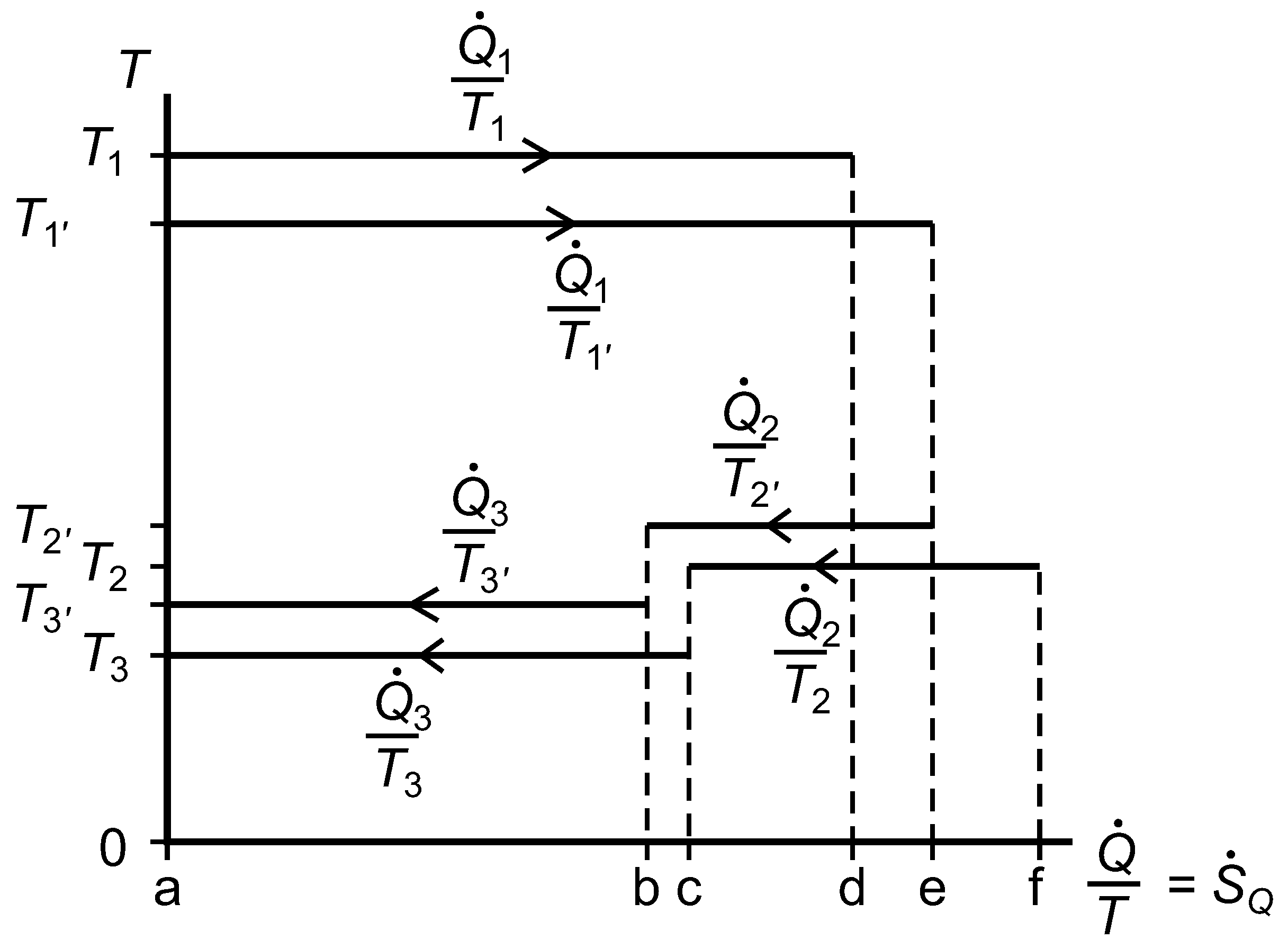
Figure 8 shows the exergy transfer rates between the subsystems of System B. System A has one exergy input rate, ${\dot{X}}_{\mathrm{in}\mathrm{A},0}$, and two exergy output rates, $\dot{W}$ and ${\dot{X}}_{{\mathrm{in}R}_0,0}$. We refer to this as a bifurcation of the exergy transfer rate path. The relative magnitudes of the exergy output rates of System A are characterized by their exergetic furcation factors; Equations (50) and (51).

$$f_{\mathrm{out}\mathrm{A},\dot{W},0}=\frac{{\dot{X}}_{\mathrm{out}\mathrm{A},\dot{W},0}}{{\dot{X}}_{\mathrm{out}\mathrm{A},\dot{Q},0}+{\dot{X}}_{\mathrm{out}\mathrm{A},\dot{W},0}}=\frac{T_{0^{\prime }}-T_{1^{\prime }}}{T_0-T_{1^{\prime }}}=\frac{[{\dot{Q}}_1{R}_1-T_1][{\dot{Q}}_1(R_0+R_1)+T_0-T_1]}{[{\dot{Q}}_1(R_0+R_1)-T_1]({\dot{Q}}_1{R}_1+T_0-T_1)}$$

(50)

$$f_{\mathrm{out}\mathrm{A},{\dot{Q}}_0,0}=\frac{{\dot{X}}_{\mathrm{out}\mathrm{A},\dot{Q},0}}{{\dot{X}}_{\mathrm{out}\mathrm{A},\dot{Q},0}+{\dot{X}}_{\mathrm{out}\mathrm{A},\dot{W},0}}=\frac{T_0-T_{0^{\prime }}}{T_0-T_{1^{\prime }}}=\frac{{\dot{Q}}_1{R}_0{T}_0}{[{\dot{Q}}_1(R_0+R_1)-T_1]({\dot{Q}}_1{R}_1+T_0-T_1)}$$

(51)

Figure 8. A diagram of the exergy transfer rates for the reversible heat engine linked by thermal resistances to two isothermal reservoirs, one of which is at the environmental temperature, $T_0$.

Figure 8. A diagram of the exergy transfer rates for the reversible heat engine linked by thermal resistances to two isothermal reservoirs, one of which is at the environmental temperature, $T_0$.

The overall rational efficiency of System B is expressed in terms of two subsystem rational efficiencies (the second of which is unity in this case) and one exergetic furcation factor; Equation (52). We note that we can complete the entire analysis of System B and its subsystems, provided we have enough information to draw the temperature versus entropy transfer rate diagram of Figure 7.

$${\eta }_{\mathrm{B},0}={\eta }_{R_1,0}·{\eta }_{\mathrm{A},0}·f_{\mathrm{out}\mathrm{A},\dot{W},0}$$

(52)

2.8. An Irreversible System Linked to Its Heat Source and Sink by Thermal Resistances

System B of Section 2.6 and Section 2.7 is a prototype of a plant or device that is thermodynamically irreversible, but can serve as a heat engine or a reverse heat engine. It exchanges heat at two temperature levels only and has a net work rate. It is characterized by its rational efficiency that is known over the ranges of its main operating parameters; Equations (36)–(39). The thermal resistances need not be linear, and their exact nature will determine the performance characteristics of the plant. In practice, the hot part of such an engine needs to be separated from the cold part, and the system boundary should be adiabatic between them. System A, within System B, could be replaced by another system like B or by an arbitrary system incorporating an appropriate cycle, such as an irreversible Carnot cycle, Stirling cycle or non-superheated regenerative Rankine cycle. Equation (52) would still apply, but ${\eta }_{\mathrm{A},0}$ would be less than unity.

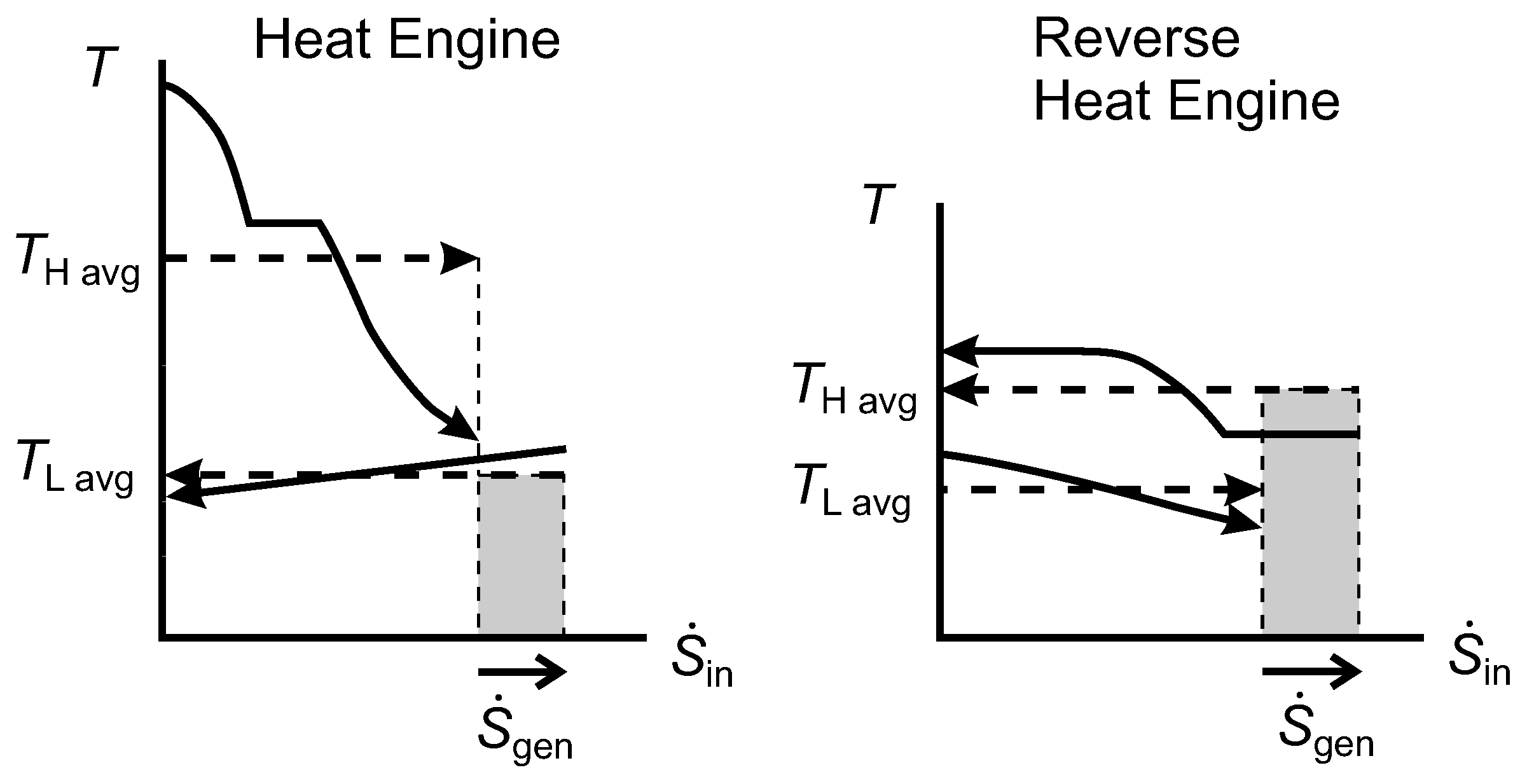
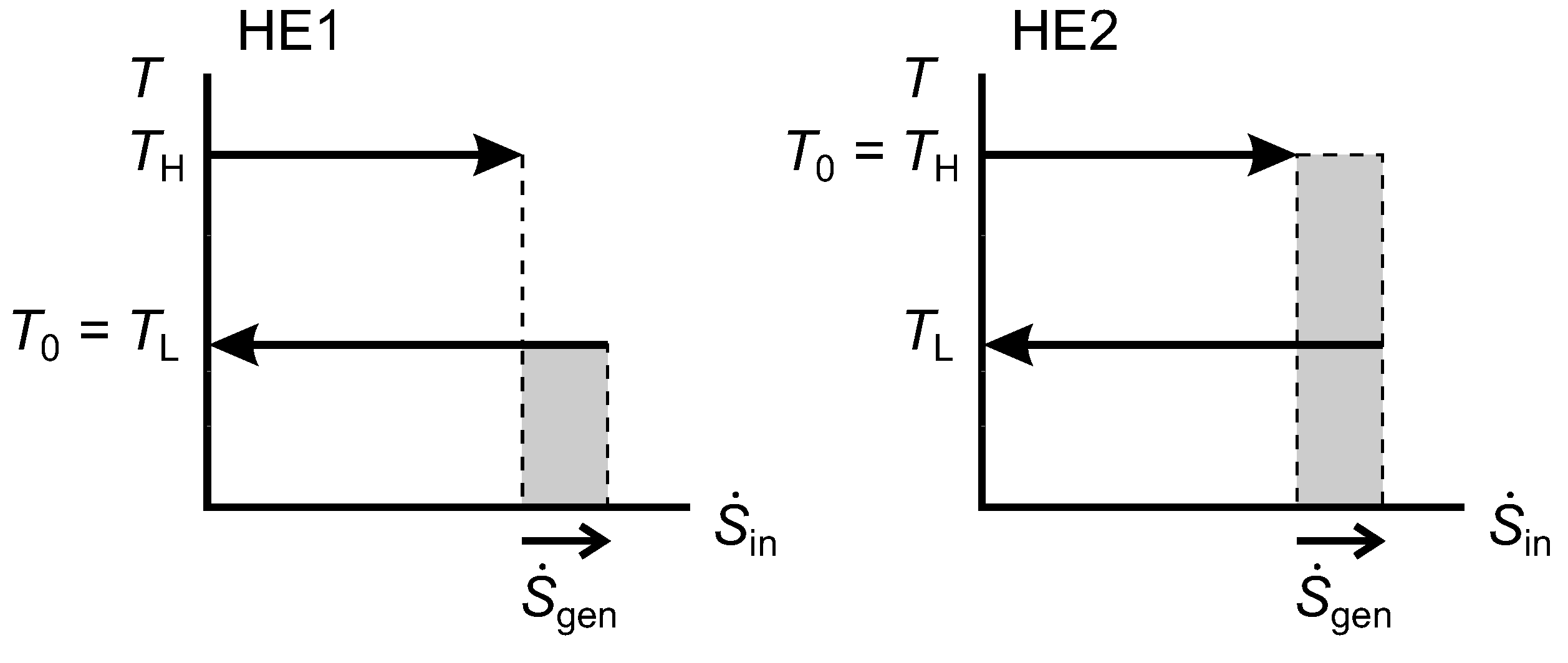
2.9. Lost Work Rate and the $T-\dot{S}$ Diagram

Figure 9 shows $T-\dot{S}$ diagrams for an irreversible HE1 and an irreversible HE2 that each have one isothermal source and one isothermal sink. In both cases, the width of the shaded area gives the rate of entropy generation, which is positive. For HE1, we can show that the shaded rectangle is the lost work rate, as follows:

$$\begin{array}{cc}\hfill {\dot{S}}_{\mathrm{gen}}{T}_{\mathrm{L}}& ={\dot{Q}}_{\mathrm{L},\mathrm{out}}-\frac{T_{\mathrm{L}}}{T_{\mathrm{H}}}{\dot{Q}}_{\mathrm{H},\mathrm{in}}\hfill \\ & ={\dot{Q}}_{\mathrm{L},\mathrm{out}}-{\dot{Q}}_{\mathrm{H},\mathrm{in}}+{\dot{Q}}_{\mathrm{H},\mathrm{in}}(T_{\mathrm{H}}-T_{\mathrm{L}})/T_{\mathrm{H}}\hfill \\ & =-{\dot{W}}_{\mathrm{net},\mathrm{out}}+{\dot{W}}_{\mathrm{net},\mathrm{out},\mathrm{rev}}={\dot{W}}_{\mathrm{net},\mathrm{out},\mathrm{rev}}-{\dot{W}}_{\mathrm{net},\mathrm{out}}={\dot{W}}_{\mathrm{lost},\mathrm{L}}={\dot{W}}_{\mathrm{lost},0}\hfill \end{array}$$

(53)

Figure 9. $T-\dot{S}$ Diagrams for an irreversible Heat Engine 1 (HE1) and an irreversible HE2.

Figure 9. $T-\dot{S}$ Diagrams for an irreversible Heat Engine 1 (HE1) and an irreversible HE2.

For HE2, the same expression for ${\dot{W}}_{\mathrm{lost},\mathrm{L}}$ applies, and we can obtain ${\dot{W}}_{\mathrm{lost},\mathrm{H}}$ using Equation(29). Hence,

$${\dot{W}}_{\mathrm{lost},0}={\dot{W}}_{\mathrm{lost},\mathrm{H}}=\frac{T_{\mathrm{H}}}{T_{\mathrm{L}}}{\dot{W}}_{\mathrm{lost},\mathrm{L}}$$

(54)

and we note that this is equal to the shaded area for HE2.

From Equation (31) for both HE1 and HE2, we see that ${\dot{S}}_{\mathrm{gen}}{T}_{\mathrm{L}}={\dot{A}}_{\mathrm{L},\mathrm{L}}$ (the shaded area shown for HE1) and that ${\dot{S}}_{\mathrm{gen}}{T}_{\mathrm{H}}={\dot{A}}_{\mathrm{L},\mathrm{H}}$ (the shaded area shown for HE2). In HE1, the reservoir at $T_{\mathrm{L}}$ is the environmental thermal reservoir, so $T_{\mathrm{L}}$ would correspond to $T_0$ in our notation for Figure 3, while $T_{\mathrm{H}}$ would correspond to $T_1$. In HE2, $T_{\mathrm{H}}$ is the environmental temperature and $T_{\mathrm{L}}$ would correspond to $T_1$.

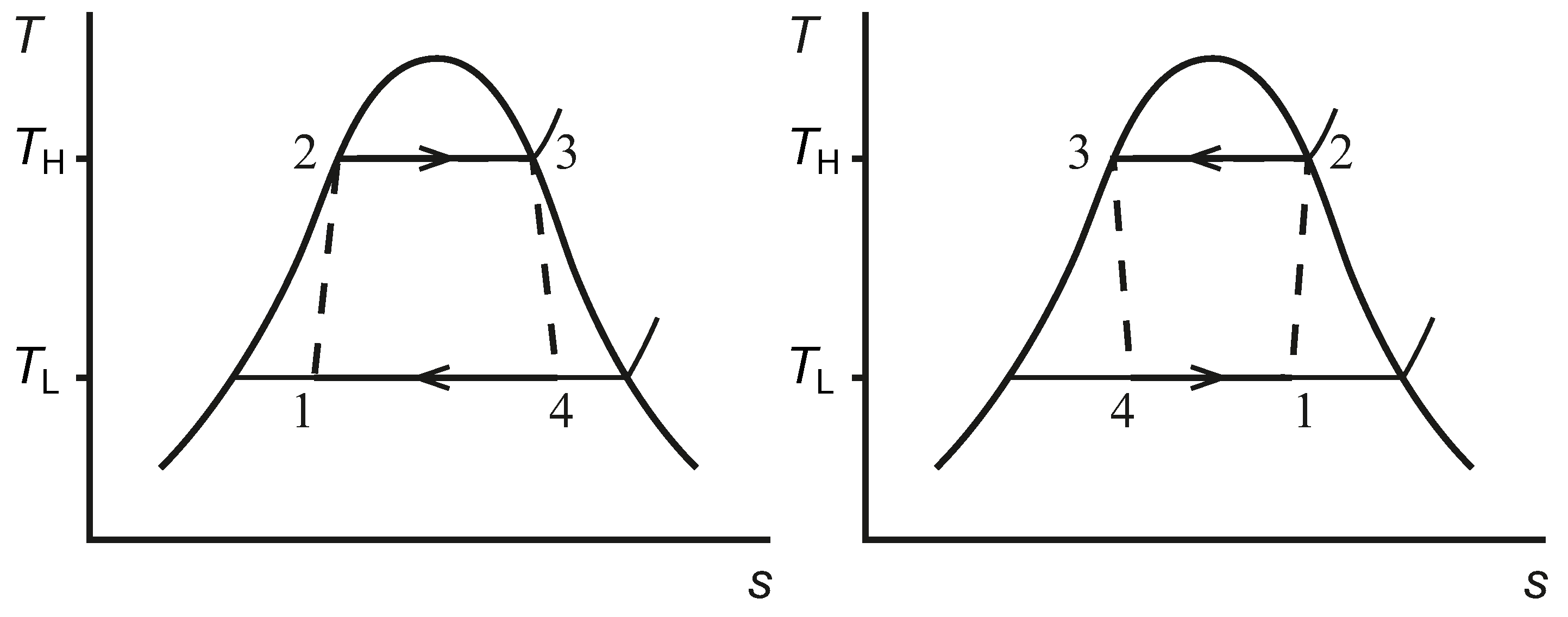
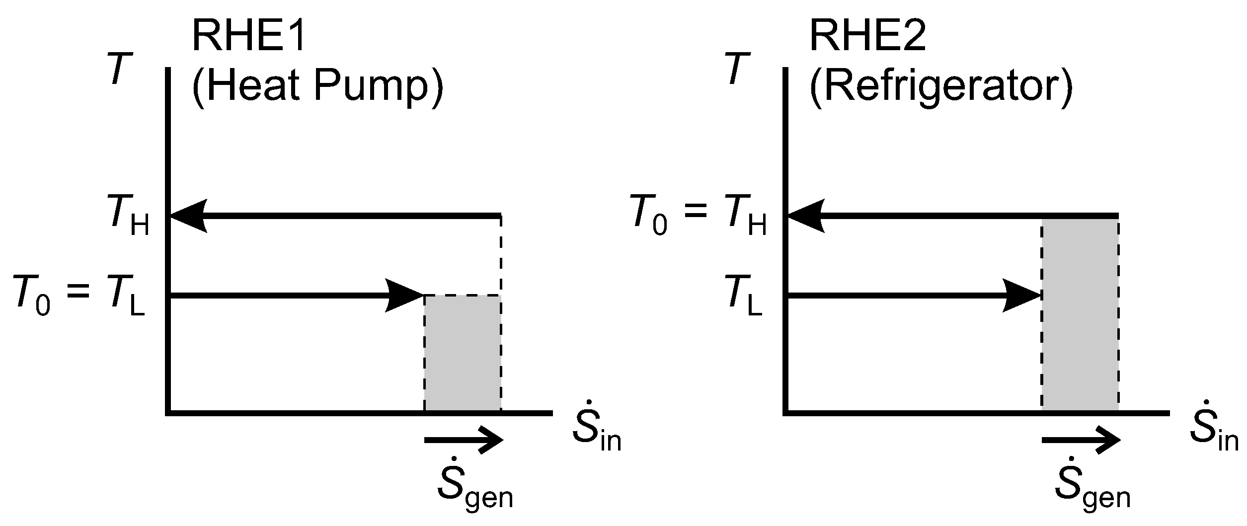
Similarly, for the reverse heat engines represented in Figure 10, we show that the shaded region for RHE2 is equal to the lost work rate for it.

Figure 10. $T-\dot{S}$ Diagrams for an irreversible Reversed Heat Engine 1 (RHE1) and an irreversible RHE2.

Figure 10. $T-\dot{S}$ Diagrams for an irreversible Reversed Heat Engine 1 (RHE1) and an irreversible RHE2.

$$\begin{array}{cc}\hfill {\dot{S}}_{\mathrm{gen}}{T}_{\mathrm{H}}& ={\dot{Q}}_{\mathrm{H},\mathrm{out}}-\frac{T_{\mathrm{H}}}{T_{\mathrm{L}}}{\dot{Q}}_{\mathrm{L},\mathrm{in}}\hfill \\ & ={\dot{Q}}_{\mathrm{H},\mathrm{out}}-{\dot{Q}}_{\mathrm{L},\mathrm{in}}+{\dot{Q}}_{\mathrm{L},\mathrm{in}}(T_{\mathrm{L}}-T_{\mathrm{H}})/T_{\mathrm{L}}\hfill \\ & ={\dot{W}}_{\mathrm{net},\mathrm{in}}-{\dot{Q}}_{\mathrm{L},\mathrm{in}}\frac{T_{\mathrm{H}}-T_{\mathrm{L}}}{T_{\mathrm{L}}}\hfill \\ & ={\dot{W}}_{\mathrm{net},\mathrm{in}}-\frac{{\dot{Q}}_{\mathrm{L},\mathrm{in}}}{\left(T_{\mathrm{L}}\right)/(T_{\mathrm{H}}-T_{\mathrm{L}})}\hfill \\ & ={\dot{W}}_{\mathrm{net},\mathrm{in}}-{\dot{W}}_{\mathrm{net},\mathrm{in},\mathrm{rev}}={\dot{W}}_{\mathrm{lost},\mathrm{H}}={\dot{W}}_{\mathrm{lost},0}\hfill \end{array}$$

(55)

For RHE1, the same expression for ${\dot{W}}_{\mathrm{lost},\mathrm{H}}$ applies, and we can obtain ${\dot{W}}_{\mathrm{lost},\mathrm{L}}$ using Equation (29). Hence,

$${\dot{W}}_{\mathrm{lost},0}={\dot{W}}_{\mathrm{lost},\mathrm{L}}=\frac{T_{\mathrm{L}}}{T_{\mathrm{H}}}{\dot{W}}_{\mathrm{lost},\mathrm{H}}$$

(56)

and we note that this is equal to the shaded area for RHE1.

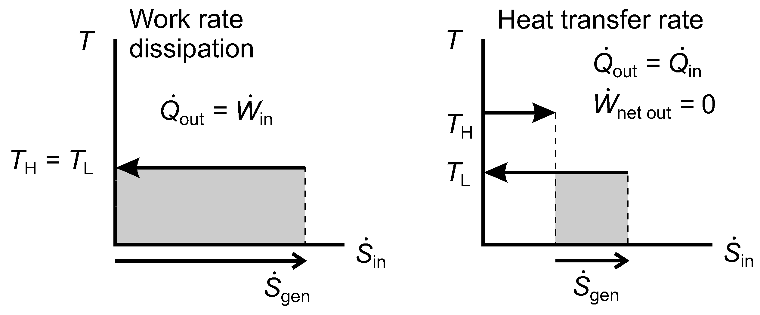
We note three special or limiting cases of the diagrams in Figure 9 and Figure 10. They do not pose any difficulties for the methodology, but is is helpful to be aware of them.

• A reverse heat engine can operate between thermal reservoirs at $T_{\mathrm{L}}$ and $T_{\mathrm{H}}=T_0$, but with only an infinitesimal heat transfer rate at $T_{\mathrm{L}}$ (regarded as a highly irreversible refrigerator), or at $T_{\mathrm{L}}$ again when $T_{\mathrm{L}}=T_0$ (regarded as a highly irreversible heat pump), Figure 10.
• There can be a net rate of work input accompanied by a corresponding net rate of heat rejection at $T_0$, e.g., a brake or a churn; Figure 11, work rate dissipation.
• There can be internal heat transfer through the system in the direction from the hotter surface to the colder one with zero net work output (a thermal resistance); Figure 11, heat transfer rate.

Externally, case 2 is infinitesimally different to case 1. Internally, the systems would differ. The highly irreversible heat pump or refrigerator would maintain a thermal gradient within the system, and part of the exergy destruction rate would be associated with internal heat conduction through that gradient, the remainder being associated with irreversibility in the reverse heat engine, also giving rise to internal heat conduction. In a fluid brake or dry friction brake, the exergy destruction rate would be associated with mechanical friction, giving rise to internal heat conduction. In an eddy current brake, the exergy destruction rate would be associated with electrical resistance, also giving rise to internal heat conduction.

Figure 11. Diagrams of temperature versus entropy transfer rates for irreversible work rate dissipation, as in a brake, and heat transfer rate in a thermal resistance.

Figure 11. Diagrams of temperature versus entropy transfer rates for irreversible work rate dissipation, as in a brake, and heat transfer rate in a thermal resistance.

3. The Environmental Temperature and Multiple Isothermal Reservoirs

Exergy analysis is built on the assumption of an enclosing environment that has a temperature that is at least approximately constant, and much consideration has been given to the concept of the environmental dead state [23,24]. Here, we use the configuration of Figure 1 to explore the meaning of $T_0$.

3.1. One Heat Source and Two Environmental Heat Sinks

We now consider System A, as in Figure 1, with one heat source at $T_1$ and two environmental thermal reservoirs at temperatures $T_2$ and $T_3$. As a concrete real-world example, heat rejection could occur from a heat engine to ambient air at 25 ${}^{\circ }$C and to seawater at 13 ${}^{\circ }$C. We use the term ‘environmental’ thermal reservoir to signify that any heat transfer with that reservoir has no intrinsic value, other than balancing the energy inputs and outputs of the steady or cyclic system in accordance with the first and second laws of thermodynamics. We assume the environmental thermal reservoirs are adiabatically separated from each other. For the present, we assume that both are heat sinks, i.e., they accept heat transfer, and that both $T_2$ and $T_3$ are lower than $T_1$. For now, also, we assume that System A is reversible.

As the environmental heat sink temperatures are not the same, neither of them can be considered the unique environmental reference temperature. We call upon a virtual isothermal reservoir to fulfil that role, and in order for it to be virtual, we impose the constraint that its net rate of heat transfer to or from System B is zero. We can imagine that this virtual reservoir connects to a point along resistance $R_2$ or a point along resistance $R_3$ and shares the effective environmental temperature, $T_0$, with that point. Our task now is to quantify that temperature.

Figure 12 is a plot of temperature versus the cumulative entropy transfer rates for the boundaries of Systems A and B. The area underneath any horizontal line on the diagram represents a rate of heat transfer through a boundary at the corresponding temperature. The total heat rejection rate from System B is given by Equation (57), and this must equal $T_0{\dot{S}}_{\mathrm{out}}$, as indicated in Equation (58). This result can be generalized for multiple ‘environmental’ isothermal reservoirs or for an environmental heat sink that involves a temperature glide, as shown in Equation (59). The integration is performed over the regions of the system where environmental entropy transfer takes place and over time.

Figure 12. A diagram of temperature versus entropy transfer rates for a reversible heat engine linked by thermal resistances to one heat source and two “environmental” heat sinks.

Figure 12. A diagram of temperature versus entropy transfer rates for a reversible heat engine linked by thermal resistances to one heat source and two “environmental” heat sinks.

$${\dot{Q}}_0=T_3{\dot{S}}_{\mathrm{ac}}+T_2{\dot{S}}_{\mathrm{cf}}$$

(57)

$$T_0=\frac{T_3{\dot{S}}_{\mathrm{ac}}+T_2{\dot{S}}_{\mathrm{cf}}}{{\dot{S}}_{\mathrm{af}}}$$

(58)

$$T_0=\frac{\int T_{\mathrm{env}}\mathrm{d}{\dot{S}}_{\mathrm{env}}}{\int \mathrm{d}{\dot{S}}_{\mathrm{env}}}$$

(59)

We note, however, that $T_0$ as defined in Equations (58) and (59) is also the average temperature of entropy rejection from the entire composite System B.

3.2. Generalization for Multiple Thermal Reservoirs

Now, we apply a technique like the one that Clausius used for cycles described on a thermodynamic state diagram, which we mentioned in Section 1.1. Rather than imagining thin Carnot cycle strips on a $p-V$ diagram, we imagine thin 3D bi-thermal (interacting with two isothermal reservoirs) closed, steady or cyclic systems. By aggregating them side-by-side, we can construct an arbitrary multi-thermal closed, steady or cyclic system. Each bi-thermal element of the side-by-side aggregation of subsystems has a hot surface, a cold surface and surfaces that are adiabatic. We can arrange them so that our composite system operates with a range of high and low temperatures distributed over the composite surface. The inequality of Clausius applies to our composite system where the integral is performed over the composite external surface and over time. We note that while the surface distribution of temperature over the cumulative entropy transfer rate is of key importance, the manner in which different thermal zones are arranged over the surface is incidental. This is not a system that we ever intend to build, but it can represent any arbitrary closed, steady or cyclic system. We have thus shown that for thermodynamic analysis, the real system can be represented as a collection of bi-thermal, adiabatically-isolated subsystems, which could have identical first and second law performance parameters. We point out that the subsystems we describe here need have no similarity to the actual component subsystems of the real system. Thus, all of the expressions and the $T-\dot{S}$ diagram that we have already described for bi-thermal steady, closed or cyclic systems apply for each of the bi-thermal subsystems.

3.3. The Nature of the Environmental Reference Temperature

We propose the following generalization of the definition of $T_0$. Our first realization is that the generalized System B, surrounded by many thermal reservoirs, is characterized by two temperatures, $T_{\mathrm{H}\mathrm{avg}}$ and $T_{\mathrm{L}\mathrm{avg}}$, the equivalent average high and low temperatures of the boundary at which the entropy acceptance and entropy rejection rates occur, as defined in Equations (60)–(65). One of these temperatures is associated with one of more “resources” (thermal sources of exergy), while the other is associated with an “environment”. Typically, the environment is our environment, assumed to be at a constant temperature.

$${\dot{Q}}_{{\mathrm{in}}^{-}}=\sum _{\forall i}\max \left(-{\dot{Q}}_i,0\right)$$

(60)

$${\dot{S}}_{{\mathrm{in}}^{-}}=\sum _{\forall i}\max \left(\frac{-{\dot{Q}}_i}{T_i},0\right)$$

(61)

$$T_{\mathrm{L}\mathrm{avg}}=\frac{{\dot{Q}}_{{\mathrm{in}}^{-}}}{{\dot{S}}_{{\mathrm{in}}^{-}}}$$

(62)

We point out that ${\dot{Q}}_{{\mathrm{in}}^{-}}$ is the rate of heat rejection from the system if the system is steady or the average rate over a cycle. Likewise, ${\dot{S}}_{{\mathrm{in}}^{-}}$ is the rate of entropy rejection from the system if it is steady or the average rate over a cycle. $T_{\mathrm{L}\mathrm{avg}}$ is thus the average temperature at which entropy rejection occurs from the system. Furthermore, $T_{\mathrm{H}\mathrm{avg}}$ is the average temperature at which entropy transfer occurs into the system.

$${\dot{Q}}_{{\mathrm{in}}^{+}}=\sum _{\forall i}\max \left({\dot{Q}}_i,0\right)$$

(63)

$${\dot{S}}_{{\mathrm{in}}^{+}}=\sum _{\forall i}\max \left(\frac{{\dot{Q}}_i}{T_i},0\right)$$

(64)

$$T_{\mathrm{H}\mathrm{avg}}=\frac{{\dot{Q}}_{\mathrm{in}}}{{\dot{S}}_{{\mathrm{in}}^{+}}}$$

(65)

The first law energy balance, Equation (27), can also be written as Equation (66). If ${\dot{Q}}_{{\mathrm{in}}^{+}}>{\dot{Q}}_{{\mathrm{in}}^{-}}$, then ${\dot{W}}_{\mathrm{net}\mathrm{out}}>0$; the system is a normal heat engine, and from the Clausius inequality, $T_{\mathrm{H}}>T_{\mathrm{L}}$. If ${\dot{Q}}_{{\mathrm{in}}^{+}}<{\dot{Q}}_{{\mathrm{in}}^{-}}$, then ${\dot{W}}_{\mathrm{net}\mathrm{out}}<0$; the system is a reverse heat engine, and once again, $T_{\mathrm{H}}>T_{\mathrm{L}}$. In steady state, or over the duration of one cycle, there is no net work output if $T_{\mathrm{H}}=T_{\mathrm{L}}$, i.e., if there is no difference between the average temperatures at which entropy is accepted and rejected.

$${\dot{Q}}_{{\mathrm{in}}^{+}}-{\dot{Q}}_{{\mathrm{in}}^{-}}={\dot{W}}_{\mathrm{net}\mathrm{out}}$$

(66)

From our consideration of the entropy generation rate of the irreversible heat engine and the irreversible reverse heat engine in Section 2.9, we conclude that for ‘above ambient’ devices (HE1 and RHE1) the environmental reference temperature of the Gouy–Stodola theorem, $T_0$, is the same as $T_{\mathrm{L}\mathrm{avg}}$, the average temperature of entropy transfer out of the overall system, as evaluated over its boundary. Thus, $T_{0\mathrm{HE}1}=T_{\mathrm{L}\mathrm{avg}}$ and $T_{0\mathrm{RHE}1}=T_{\mathrm{L}\mathrm{avg}}$. For ‘below ambient’ devices, $T_{0\mathrm{HE}2}=T_{\mathrm{H}\mathrm{avg}}$ and $T_{0\mathrm{RHE}2}=T_{\mathrm{H}\mathrm{avg}}$.

We now propose Equation (67), where the left-hand side is the sum of the net exergy and anergy transfer rates into a closed steady or cyclic system, which combines the Clausius inequality, Equations (25) and (26) and the Gouy–Stodola theorem, Equation (28). In this equation, our use of the terms exergy and anergy is consistent with Rant’s original usage [13], but is more restricted. Rather than expressing the exergy and anergy of an amount of energy, we use a time rate form and determine the exergy and anergy transfer rates corresponding to energy transfer rates across the boundary of a closed, steady or cyclic system. The net energy input rate equals the sum of the net exergy and anergy input rates, and this equation is equivalent to Equation (27) (a first law statement).

$${\dot{X}}_{\mathrm{in}}+{\dot{A}}_{\mathrm{in}}=0$$

(67)

The net rate of anergy input is given by Equation (68), and the net rate of exergy input associated with heat transfer is given by Equation (69). The net exergy transfer rate associated with work equals the work transfer rate and has the same direction as it; Equation (70).

$${\dot{A}}_{\mathrm{in}}=T_0{\dot{S}}_{\mathrm{in}}=T_0\sum _{\forall i}\frac{{\dot{Q}}_i}{T_i}$$

(68)

$${\dot{X}}_{\mathrm{in}\dot{Q}}=\sum _{\forall i}(T_i-T_0)\frac{{\dot{Q}}_i}{T_i}=\sum _{\forall i}(T_i-T_0){\dot{S}}_i={\dot{Q}}_{\mathrm{in}}-T_0\sum _{\forall i}\frac{{\dot{Q}}_i}{T_i}$$

(69)

$${\dot{X}}_{\mathrm{in},\dot{W}}={\dot{W}}_{\mathrm{net}\mathrm{in}}=-{\dot{W}}_{\mathrm{net}\mathrm{out}}$$

(70)

Hence, we can re-write Equation (67) as Equation(71).

$${\dot{W}}_{\mathrm{net}\mathrm{in}}+\sum _{\forall i}(T_i-T_0)\frac{{\dot{Q}}_i}{T_i}+T_0\sum _{\forall i}\frac{{\dot{Q}}_i}{T_i}=0$$

(71)

We note that the addition of the net rate of exergy input to $T_0$ times the left-hand side of the Clausius inequality converts it to an equality (which loses its second law nature, as the ${\dot{Q}}_i/T_i$ terms cancel). However, we can express the second law of thermodynamics using a ‘greater than zero’ inequality as Equation (72) or, in more detail, as Equation (73).

$${\dot{X}}_{\mathrm{in}}\ge 0$$

(72)

$${\dot{W}}_{\mathrm{net}\mathrm{in}}+\int (T-T_0)\frac{\mathrm{d}{\dot{Q}}_{\mathrm{in}}}{T}\ge 0$$

(73)

where $T_0$ is defined by Equation (74) or Equation (75), as appropriate.

$$T_0=\frac{\int \mathrm{d}{\dot{Q}}_{{\mathrm{in}}^{-}}}{\int \frac{\mathrm{d}{\dot{Q}}_{{\mathrm{in}}^{-}}}{T}}\mathrm{for}\mathrm{HE}1\mathrm{or}\mathrm{RHE}1$$

(74)

$$T_0=\frac{\int \mathrm{d}{\dot{Q}}_{{\mathrm{in}}^{+}}}{\int \frac{\mathrm{d}{\dot{Q}}_{{\mathrm{in}}^{+}}}{T}}\mathrm{for}\mathrm{HE}2\mathrm{or}\mathrm{RHE}2$$

(75)

4. Methodology Suggestions

We have shown that for a closed, steady or cyclic system, the average rate of exergy destruction, also known as the lost work rate or the irreversibility rate, can be evaluated and the rational efficiency of the system calculated. If we can partition the overall system into subsystems that are also closed and steady or cyclic, then we can evaluate the average rates of exergy destruction and the rational efficiencies of those subsystems, as well.

In practice, we may obtain the distribution of heat flux and temperature over the surface in various ways: through measurement, simulation of the system and its surroundings (using all of the techniques of mechanics, fluid mechanics, heat transfer, theory of electromagnetism, etc.), estimation or a combination of these. If we have a thermal map of the surface and a map of the heat flux into the surface (positive and negative), over the entire surface of the boundary, then from the first law of thermodynamics, we also know the net rate of work transfer into or out of the system. As an example of the use of experimentation and estimation we provide reference [25], which describes non-intrusive performance testing of a domestic freezer conducted by Oladunjoye and second law analysis by McGovern.

Figure 13. Example diagrams of temperature versus entropy transfer rates for closed, steady or cyclic systems.

Figure 13. Example diagrams of temperature versus entropy transfer rates for closed, steady or cyclic systems.

We suggest that the diagram of temperature versus cumulative entropy transfer rate into the surface is a useful tool for the analysis. Figure 9 and Figure 10 are the simplest case examples. The incremental ‘amounts’ of heat transfer rate through the boundary can be sorted, and the resulting overall diagrams for a heat engine or a reverse heat engine might be as shown in Figure 13. We define $T_0$ strictly on the basis of the overall boundary. When analysing exergy flows within the overall analysis boundary, we also use $T_0$ of the overall boundary for calculating the exergy transfer rates at the subsystem boundaries. In most cases, we extend the overall analysis boundary into the real physical environment of the plant, but in some cases, the effective environment could involve various temperature glides or levels. Furthermore, the method would allow cyclic variations in the environmental temperature to be taken into account, e.g., diurnal temperature variations.

5. The Irreversible Carnot System of Finite Thermal Resistance

We denote any system of the type shown in Figure 2 as a reversible Carnot system, as it corresponds to the class of systems that Carnot described in 1824 [9]. This class could employ a vapour (two phase), gaseous, liquid or solid medium—Carnot indicated he did not favour liquid or solid. He specified that only infinitesimal temperature differences for heat transfer should subsist in his ideal heat engine. Thus, the working medium would have only infinitesimal thermal resistance, or would require infinite time to produce a finite net work output. Carnot also clearly stated that all temperature changes within the working medium were to be due to compression and expansion only. He wrote, “We have shown that the character of the most effective utilization of heat in the production of movement would be that all temperature changes in the body were due to volume changes. The more we approach meeting this condition, the better the heat will be used,” ([9], p. 50, our translation). Carnot was very clear that this ideal heat engine (normal or reverse) was the limiting case for maximum performance.

Carnot may not have considered or known about the possibility of regenerative internal heat transfer, as in the prior Stirling (gas) or subsequent Malone (liquid) cycles, or the idealized cycle of today’s Rankine steam cycle plants with regenerative feed water heating, which could exist within a ‘Carnot system’. His statement in relation to temperature changes of the working medium was not sufficiently general to include these cases. We propose: for each and every infinitesimal temperature range through which the temperature of the medium is increased and decreased in a reversible cycle between two isothermal reservoirs, there can be only a net external energy transfer that is entirely work. Clausius’ equality applies and is sufficient. We now elaborate the irreversible Carnot system.

Figure 14 illustrates an irreversible Carnot cycle and an irreversible reverse Carnot cycle on a state diagram of temperature versus specific entropy. There is no regenerative internal heat transfer. We can imagine a system that undergoes this cycle, such as Carnot’s Figure 1 ([9], p. 17). For the normal heat engine or the reverse engine to be reversible, the adiabatic compression and expansion processes (the dashed lines in Figure 14) would have to be vertical, which would correspond to Carnot’s ideal. If these are irreversible, entropy must increase in each. It seems to us that the possible mechanisms of irreversibility, such as mechanical friction, fluid friction, electrical resistance and, of course, temperature differences within the body of the medium while it is being expanded or compressed, all require the presence of thermal resistance, and will not involve any irreversibility otherwise. If the thermal resistance of the working substance is low or infinitesimal then no continuous amount of that medium can be allowed to contact the high and low temperature reservoirs at the same time. As an aside, perhaps this gives us a clue as to how one might construct an electrically and thermally superconducting, reversible thermoelectric device: the arrangement might involve energy storage and switching. We propose therefore that finite thermal resistance is an inherent characteristic of the irreversible Carnot system, just as infinitesimal thermal resistance is mandatory for a reversible Carnot system.

Figure 14. Temperature versus specific entropy diagrams for irreversible Carnot cycles undergone by a two phase working fluid. For a normal heat engine the sense is clockwise, while for an reverse heat engine the sense is anticlockwise.

Figure 14. Temperature versus specific entropy diagrams for irreversible Carnot cycles undergone by a two phase working fluid. For a normal heat engine the sense is clockwise, while for an reverse heat engine the sense is anticlockwise.

The Curzon Ahlborn system, B in Figure 3, is an instance of an irreversible Carnot system. Based on what happens at its boundary (as distinct from its internal structure), the irreversible Carnot system is indistinguishable from the Curzon Ahlborn system. Also, the way in which the two resistances of the Curzon Ahlborn system are apportioned between $R_1$ and $R_0$ is immaterial ($R=R_0+R_1$). Figure 9 and Figure 10 apply for an irreversible Carnot system, just as they do for a Curzon Ahlborn system. The irreversible Carnot system has a characteristic thermal resistance that is given by the same expressions as apply for the Curzon Ahlborn system, Equations (76) and (77). We derived these expressions from Equations (36) and (38). In Figure 15, we summarize how the rational efficiency implies the resistance, or vice versa. There is no implication that the real system has a single thermal resistance that can be localized—it characterizes the entire distributed irreversibility.

$$R_{\mathrm{CHE}\mathrm{irr}}=\frac{(1-\eta )(T_1-T_0)T_1}{{\dot{Q}}_{\mathrm{H}\mathrm{in}}[T_1-\eta (T_1-T_0)]}$$

(76)

$$R_{\mathrm{CRHE}\mathrm{irr}}=\frac{(1-\eta )(T_1-T_0)T_1}{{\dot{Q}}_{\mathrm{H}\mathrm{out}}(T_1-T_0-\eta T_1)}$$

(77)

Figure 15. Summary of the equivalence of an irreversible Carnot system having a given rational efficiency relative to $T_0$ and a Curzon Ahlborn system having a certain resistance

Figure 15. Summary of the equivalence of an irreversible Carnot system having a given rational efficiency relative to $T_0$ and a Curzon Ahlborn system having a certain resistance

6. Overall and Subsystem Rational Efficiencies

Whenever we evaluate a rational efficiency for an overall closed, steady or cyclic plant there is the presumption that, in principle, the plant could be replaced with a perfect thermodynamic device that would have a rational efficiency of unity when interacting with the same exergetic resource and the same environment. The rate of exergy supply from the exergetic resource is always positive. The exegetic resource may be a thermal reservoir with an ‘above ambient’ effective temperature, or one with a ‘below ambient’ effective temperature. In the first case the rate of heat transfer from that resource can be specified as a positive fraction of the heat transfer rate from the resource, while in the second case the rate of heat transfer from the resource is a negative quantity and the rate of exergy transfer can be expressed as a negative fraction of it. Otherwise, the exergetic resource is a source of a positive rate of work. The environment will have an effective temperature for the supply or acceptance of an entropy transfer rate (which we can express as a heat transfer rate or anergy flow by multiplying the entropy transfer rate by $T_0$).

From the balances we have examined in detail, the perfect device differs from the real plant: it exchanges entropy, heat or anergy with the environment at a lower rate. Therefore the nature of the reference environment must be such that it does not constrain the rate of entropy transfer to or from itself. When we widen the analysis boundary, as we conventionally do in exergy analysis, we are ensuring this freedom from constraint. By doing so, we acknowledge the constraints that actually exist. For a closed, steady or cyclic system that undergoes no net change this constraint is associated with thermal resistance.

Considering System B in Figure 1 to be a subsystem of some overall system, its rational efficiency quantifies how efficiently energy transformations between heat transfer rates and a net work rate in either direction are brought about. More generally, the transformations can be between two or more exergy transfer rates, where the exergy transfer rates can be associated with net heat transfer rates at specified temperature levels or a net work rate. If the exergetic resource is thermal, certain of the isothermal reservoirs are receiving a flow of exergy directly or indirectly from it; others may be supplying flows of exergy to thermal exergy sinks to meet specified demands, while the remainder are supplying or receiving anergy directly or indirectly to or from the environment. If the exergetic resource is one that is providing a rate of work, some of the isothermal reservoirs are providing rates of exergy output to thermal exergy sinks to meet specified demands, while the remainder are supplying or receiving anergy directly or indirectly to or from the environment.

Without knowledge of the effective temperature of the environment it is possible to determine the rational efficiency of System B, based on the effective temperature $T_{0,\mathrm{B}}$ of those “isothermal reservoirs” (in fact, just surfaces through which heat transfer is occurring) that are neither receivers of exergy flow from the exergetic resource, nor suppliers of exergy flow directly or indirectly to exergy sinks to meet specified demands, based on the actual operating parameters. $T_{0,\mathrm{B}}$ is the constrained reference temperature of System B at this operating point. Therefore, for a particular operating point the system can be characterized by its rational efficiency and the rate and direction of anergy flow referred to $T_{0,\mathrm{B}}$ can be determined. This is very significant, as we have a way of characterizing the performance of subsystems in a way that does not depend on the temperature of the environment $T_0$. When we know the effective temperature of the environment we can complete the evaluation of the overall rational efficiency. We note that an anergy flow at the constrained reference temperature of a subsystem corresponds to an exergy flow relative to the environmental temperature. However, we also have the option of evaluating ${\dot{A}}_0$ (the anergy flow at $T_0$) directly from ${\dot{A}}_{0,\mathrm{B}}$ (the anergy flow relative to $T_{0,\mathrm{B}}$) by using Equation (31).

Valero et al. [20] identified level of aggregation as a significant aspect to be considered in the analysis of energy transforming systems. If a closed, steady or cyclic system that undergoes no net change contains flow cycles, such as the Rankine or reversed Rankine cycle, it cannot be disaggregated into closed systems that would isolate components such as a turbine, a nozzle or a condenser for closer analysis. O’Toole and McGovern [26] have shown how a net flow across a boundary owing to several streams can have an equivalent exergy transfer rate. Building on this, McGovern and O’Toole [27,28] proposed a virtual system concept that can be used to extract the network structure of exergy flows associated with complex steady flow heat engines.

7. Discussion

We present these ideas for consideration and for discussion. Real plants are complex, and we do not expect to find analytical expressions that accurately represent their performance characteristics. However, we have the means to model irreversibility in great detail if we so wish. This exploration of a simple arrangement of a closed system linked to isothermal reservoirs has enabled the isolation of some significant aspects of exergy analysis and finite time thermodynamics. Exergy analysis is not an alternative to entropy generation minimization analysis or finite-time thermodynamics methods. These approaches overlap, but are complementary.

Equation (20) has some notoriety, as it contains only two parameters and, yet, is a step closer to reality than Equation (5). The difference between these two equations is the difference between finite time and infinite time thermodynamics. In reality, thermal resistance exists. The reversible Carnot cycle system has no thermal resistance and, therefore, only models real processes that would take infinite time to complete in a reversible manner. Using Equation (12) for the Curzon and Ahlborn system, B in Figure 3, and the cost of ${\dot{Q}}_1$ in € per W, if we have the annual cost of conductance, $1/R_{\mathrm{tot}}$, in € per W/K, we can estimate an appropriate plant efficiency. Equation (20) is appropriate for a particular thermo-economic situation where maximum power is needed. It gives a reasonably good rough estimate of what is possible, on the basis that engineers currently implement working fluid cycles, such as the Rankine cycle, with a very high inherent rational efficiency. In using these equations, $T_1$ should be calculated in the manner of Equations (62) and (65).

Allowing for only a constant environmental temperature in exergy analysis is rather restrictive. We have shown that such restriction is not essential for exergy analysis. Each subsystem has its own constrained environment, and in this paper, we have provided the foundation for developing this concept.

Sometimes, the overall composite system may have one single thermal reservoir with which it interacts. The net work output rate can only be negative, and the system is an exergy destruction sink, which may seem trivial. Computer chips that consume exergy are cases in point, but overall size-and-performance optimization typically leads to a chip operating temperature that is not the same as the temperature of the environment and should therefore involve exergoeconomic analysis. Currently, large-scale data centres or computer server farms destroy exergy at a high rate, and the challenge is to minimize this. Indeed, because the temperature of the environment varies cyclically, these plants have a multi-thermal boundary. Exergoeconomic analysis is certainly appropriate.

The applications of thermodynamics generally are vast. The planet Earth is an example of a system that has a roughly cyclic temperature distribution over its surface and an associated, roughly cyclic heat flux distribution. As a simplification, its exergetic resource is the disc of the sun and its environment is the balance of a spherical shell at the cosmic background temperature. Perhaps the approach described here has some relevance to understanding it better. Likewise, could it be applied to the map of cosmic temperature and its associated heat flux distribution over time and surface?

8. Conclusions

The model of a closed reversible or irreversible system linked by constant resistances to isothermal reservoirs provides useful insights into finite time, or irreversible, thermodynamics. The temperature versus entropy transfer rate method can localize exergy destruction rates and provide subsystem rational efficiencies. Without going to extraordinary lengths, a methodical approach can be used to specify an appropriate thermal reference environment model as part of an overall exergy analysis approach, respecting the principles of finite time thermodynamics. We have shown that the reference environment need not necessarily be at a single constant temperature. By expressing the second law of thermodynamics in terms of the net exergy input rate to a closed, steady or cyclic system that undergoes no net change, we have clarified the link between the Clausius integral of heat over temperature and the reference temperature of the Gouy–Stodola theorem. We have demonstrated the equivalence of the Curzon Ahlborn system and the irreversible Carnot system. We have also outlined how subsystem rational efficiencies relate to overall rational efficiency. We have found that Rant’s anergy is in fact a very important concept for the analysis of heat and work rates over the boundary of a system. From the evidence we have presented, we postulate that heat transfer through thermal resistance is the sole basis of irreversibility.