Article

Information Theory for Correlation Analysis and Estimation of Uncertainty Reduction in Maps and Models

by
J. Florian Wellmann
CSIRO Earth Science and Resource Engineering, 26 Dick Perry Ave., Kensington 6151, WA, Australia
Entropy 2013, 15(4), 1464-1485; https://doi.org/10.3390/e15041464
Submission received: 19 February 2013 / Revised: 12 April 2013 / Accepted: 15 April 2013 / Published: 22 April 2013
(This article belongs to the Special Issue Applications of Information Theory in the Geosciences)

Abstract

:
The quantification and analysis of uncertainties is important in all cases where maps and models of uncertain properties are the basis for further decisions. Once these uncertainties are identified, the logical next step is to determine how they can be reduced. Information theory provides a framework for the analysis of spatial uncertainties when different subregions are considered as random variables. In the work presented here, joint entropy, conditional entropy, and mutual information are applied for a detailed analysis of spatial uncertainty correlations. The aim is to determine (i) which areas in a spatial analysis share information, and (ii) where, and by how much, additional information would reduce uncertainties. As an illustration, a typical geological example is evaluated: the case of a subsurface layer with uncertain depth, shape and thickness. Mutual information and multivariate conditional entropies are determined based on multiple simulated model realisations. Even for this simple case, the measures not only provide a clear picture of uncertainties and their correlations but also give detailed insights into the potential reduction of uncertainties at each position, given additional information at a different location. The methods are directly applicable to other types of spatial uncertainty evaluations, especially where multiple realisations of a model simulation are analysed. In summary, the application of information theoretic measures opens up the path to a better understanding of spatial uncertainties, and their relationship to information and prior knowledge, for cases where uncertain property distributions are spatially analysed and visualised in maps and models.

Graphical Abstract

1. Introduction

Maps and models are widely used to represent the distribution of properties in space in diverse areas ranging from studies in a geographical framework, to complex three-dimensional model analyses, to the visualisation of tomographic data in medical and material sciences. In all cases where these representations are used for further decisions, analysis and visualisation of uncertainties associated with the distribution of properties are important. Information entropy has been identified as a meaningful measure to analyse and visualise uncertainties in this spatial context [1,2]. Once significant uncertainties are identified, the logical next step is to determine how they could be reduced. In this work, it will be evaluated how measures from information theory can be applied to determine spatial correlations of uncertainty, and the possible reduction with additional information. The evaluation is outlined for the context of geoscientific information, typically presented in maps and three-dimensional models. However, the application to related problems of uncertainty quantification and analysis in other fields is straightforward.
The analysis and visualisation of uncertainties in geoscientific studies is the scope of intense research, for maps and geographic information systems (GIS) ([3,4,5,6,7]), and increasingly for three-dimensional geoscientific models ([8,9,10,11,12,13]). Information entropy has been proposed for the visualisation of spatial uncertainties in maps by Goodchild et al. [14], and more recently, the concept has successfully been applied for uncertainty quantification and analysis in complex three-dimensional structural geological models [2]. An advantage of using information entropy for uncertainty analysis is that it combines the probabilities for multiple outcomes to one meaningful measure ([15]), and that it does not assume a specific statistical distribution or an estimate of a mean [1].
Building upon the concept of information entropy to analyse spatial uncertainties, the hypothesis of this work is that additional information theoretic measures can be used for the analysis of correlations and potential reductions of uncertainties in space. Specifically, it is often of great interest to determine how additional information at one location would reduce uncertainties elsewhere. In an information theoretic framework, these questions can be addressed with joint entropy, conditional entropy, and mutual information (e.g., [15,16,17]).
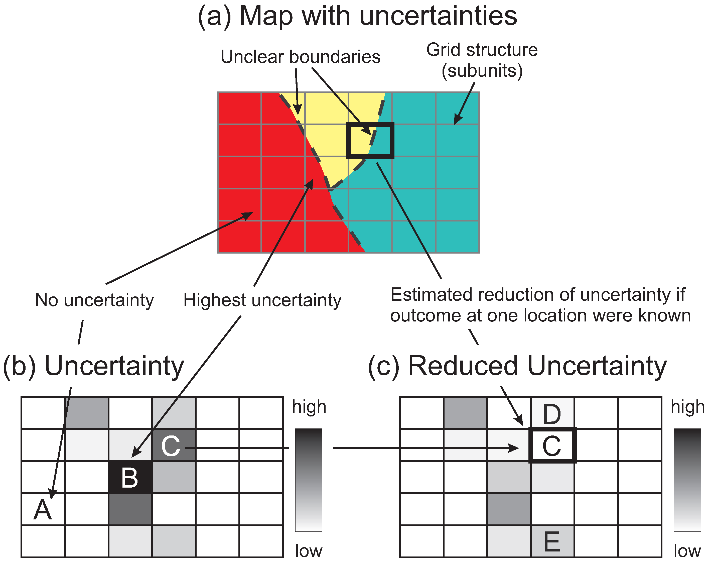
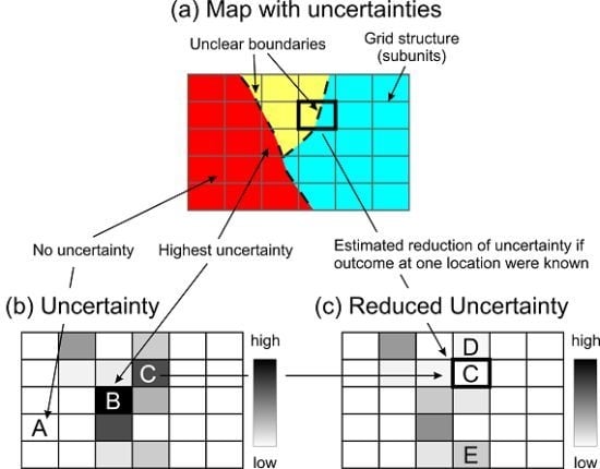
An overview of the research problem is sketched in Figure 1. Consider a case of spatial uncertainty (Figure 1a) where three distinct regions exist (for example geological units), but the location of the boundary between the regions is uncertain. In a first step, probabilities for each outcome are estimated in discrete subregions, here as cells in a regular grid. A measure of uncertainty is then applied based on the probability distributions at each location (Figure 1b): A cell with known outcome (far away from the boundary) has no uncertainty (label A), cells closer to a boundary where two outcomes are possible have a higher uncertainty, and the maximal uncertainty exists where three outcomes are probable (label B).
The relevant question of spatial uncertainty reduction investigated in this work is represented in Figure 1c, i.e., the estimation of where, and by how much, additional information at one point can be expected to reduce uncertainties elsewhere. An important aspect of the research question is that the expected reduction of uncertainty should be estimated without having to assume a specific outcome. For example, in Figure 1c, without knowing the actual outcome in one cell (e.g., label C with black outline), what would be the expected reduction of uncertainties in other cells (e.g., D and E), if we would have the information of cell C? Information entropy as a measure of uncertainty quantification, represented in Figure 1b, has been presented in [2]. The extension to additional measures of information theory to address the problem sketched in Figure 1c is evaluated here.
Figure 1. Principle of the evaluation of spatial uncertainty reduction through additional information, investigated in this work. (a) Map of three regions with uncertain boundaries (dashed lines) and cells in a regular grid used for subsequent uncertainty analysis. (b) Uncertainty estimation based on probabilities of discrete outcomes in each cell. (c) Estimated reduction of uncertainties; given the information in one cell (black outline), the remaining uncertainty within this cell is 0 and uncertainties in the surrounding cells are reduced. Adapted from Figure 2 in [2].
Entropy 15 01464 g001
In the following, the concept of using information entropy as a measure of spatial uncertainty is briefly reviewed, followed by a description of the important concepts of joint entropy, conditional entropy, and mutual information. As a test of feasibility, the measures are applied to a simple, but typical, simulation example of spatial uncertainty about the unknown depth and thickness of a geological layer of interest (for example a layer with a high mineral content, a coal layer, etc.). However, the application of the measures can be transferred to other cases where uncertainties are evaluated in a spatial context. In the case shown here, the analysis is focused on the determination of uncertainty correlations in the subsurface. In this setting, one important objective of the analysis is to answer a question that is of great relevance in many typical exploration settings: if additional information would be obtained, for example through drilling, then where, and by how much, would this additional information reduce spatial uncertainties?
Figure 2. Example model of a geological layer at depth with two types of uncertainty: (i) the depth to the top surface of the layer is uncertain; and (ii) the thickness of the layer is uncertain.
Entropy 15 01464 g002

2. Analysis of Spatial Uncertainties with Measures from Information Theory

2.1. Uncertainty of a Single Random Variable

Information entropy, originally developed in the context of coding theory and communication [18], has been applied as a measure of uncertainty in a wide range of subjects (e.g., [15,16]) as it provides an intuitive quantitative measure for the interpretation of uncertainties. This quantitative aspect is an important foundation for the interpretation of spatial correlations of uncertainty below and will therefore be outlined briefly.
The application of information entropy as a measure of spatial uncertainty is based on the premise that the desired criteria to examine uncertainties are equivalent to those in the context of information transmission. The most important aspects in the spatial context are [2]:
  • If no uncertainty exists at a specific location, then the measure is zero;
  • The measure is strictly greater than zero when uncertainty exists;
  • If several outcomes at a location are probable, and all are equally likely, then the uncertainty is maximal;
  • If an additional outcome is considered, the uncertainty cannot be lower than without this outcome;
Information entropy fulfils these criteria. The information entropy of a random variable is directly derived from the probability distribution of potential outcomes. Consider a random variable X with n possible outcomes x 1 , x n . The probability of an outcome x i n is then p ( X = x i ) , in the following abbreviated with p i . The information entropy for the random variable X is [15,18]:
H ( X ) = i = 1 n p i log 2 p i
If the information entropy is calculated with the logarithm to the base of two, as shown here, then the units of H are measured in bits (binary digits). All examples in the following are calculated to the base of two. However, other bases are possible and the results are simply transformable.
An important aspect of the information entropy is the fact that it reaches its maximum value when all outcomes are equally probable. Using the method of Lagrangian undetermined multipliers, it is straightforward to prove that, for n possible outcomes, the function has its maximum value for the uniform distribution (e.g., [17]). In the case of the n possible discrete outcomes, the maximum value of H ( X ) is therefore reached when:
p i = 1 n
and the maximum value is
H max ( X ) = i = 1 n 1 n log 2 1 n
= log 2 n
An instructive and intuitive interpretation of the information entropy can be obtained for the typical example of a coin flip with two possible outcomes, presented in the Appendix. For further details see, for example, the excellent descriptions in Cover and Thomas [15] or MacKay [16].

2.2. Interpretation in a Spatial Context: Uncertainty at a Single Location

The extension of information entropy into a spatial context follows directly from the concept that a discrete model subregion (e.g., a cell), identified with a position vector r = ( x , y , z ) , can be considered as a random variable X ( r ) with a set of n possible exclusive outcomes:
H ( X ( r ) ) = i = 1 n p i ( r ) log 2 p i ( r )
Equivalent to before, p i ( r ) is the abbreviation for p ( X ( r ) = x i ) , the probability of an outcome x i for the random variable X at position r . A detailed introduction into information entropy in the context of spatial interpretation is given in Wellmann and Regenauer-Lieb [2]. For simplification, all the following descriptions will be referring to this spatial interpretation, and the random variables will be denoted as X r X ( r ) .

2.3. Correlations of Uncertainty between Two Variables or Locations

As the aim of the presented work is to determine where additional information will lead to a reduction of uncertainties, the important next step is to evaluate correlations of uncertainty between two random variables or, in the spatial context, two discrete regions or cells. The information theoretic measures of relationships between information of variables, complementary to information entropy, are described in the following.

2.3.1. Joint Entropy

The joint entropy of two random variables X 1 and X 2 at positions r 1 and r 2 is defined as (e.g., [15,17]):
H ( X 1 , X 2 ) = i j p i j ( r 1 , r 2 ) log 2 p i j ( r 1 , r 2 )
The joint entropy for two variables (or locations, in a spatial sense considered here) can be interpreted as the information entropy of the joint probability table between both variables. It provides a measure of the overall uncertainty related to this table. An important inequality between the joint entropy and the information entropies of the single variables is
H ( X 1 , X 2 ) H ( X 1 ) + H ( X 2 )
with equality if and only if the variables X 1 and X 2 are independent (see for example [17], for a derivation).

2.3.2. Conditional Entropy

Conditional entropy is a measure of the information entropy that is expected to remain for one random variable, given the additional information of another random variable (i.e., when it is conditioned on another variable). It is derived on the basis of the conditional probability as the average entropy of a variable X 2 for all outcomes of X 1 (e.g., [15,17]):
H ( X 2 | X 1 ) = i p i ( x 1 ) H ( X 2 | X 1 = i )
The relationship between joint entropy and conditional entropy for two random variables is (e.g., [17]):
H ( X 1 , X 2 ) = H ( X 2 | X 1 ) + H ( X 1 ) = H ( X 1 | X 2 ) + H ( X 2 )
Combining Equations (8) and (6), the important inequality is obtained that additional information of another variable can only reduce entropy:
H ( X 1 , X 2 ) H ( X 1 ) + H ( X 2 )
H ( X 2 | X 1 ) + H ( X 1 ) H ( X 1 ) + H ( X 2 )
H ( X 2 | X 1 ) H ( X 2 )
with equality if and only if the two random variables are independent.

2.3.3. Mutual Information

Related to the concepts of conditional entropy and joint entropy is the measure of mutual information. It quantifies the amount of information shared between two variables and is defined by (e.g., [15,17])
I ( X 1 ; X 2 ) = H ( X 1 ) + H ( X 2 ) H ( X 1 , X 2 )
From the inequality for joint entropy (6), it follows directly that the mutual information between two random variables is always larger than or equal to zero
I ( X 1 ; X 2 ) 0
with equality, again, for the case that both variables are independent. Also important are the notions that:
I ( X 1 ; X 2 ) = I ( X 2 ; X 1 )
and
I ( X 1 ; X 1 ) = H ( X 1 )
These equations state that the mutual information between two random variables is symmetrical, and that the information entropy can be considered as a special case of mutual information, i.e., the information the variable shares with itself.

2.4. Correlations of Uncertainty between Multiple Variables

The measures for the analysis of correlations between two variables can be applied to determine how much information is shared between exactly two positions in space. However, in many realistic problems it is of interest to estimate how accumulating information at multiple other locations would lead to an overall reduction of uncertainty. As an illustration in the geoscientific context, the information that is subsequently gained when drilling a well or during a sampling campaign implies that every new observation that is obtained may reduce uncertainties further, in addition to the reduction of uncertainties due to previous observations.
For this purpose, the information theoretic concepts can be extended to a multinominal form. For a formal derivations see, for example, the descriptions in Cover and Thomas [15], MacKay [16] and Ben-Naim [17].
The joint entropy for multiple variables X 1 , X 2 , , X n can be derived from an extension of Equation (5) as:
H ( X 1 , X 2 , , X n ) = i 1 , i 2 , , i n p i 1 , i 2 , , i n ( r 1 , r 2 , , r n ) log 2 p i 1 , i 2 , , i n ( r 1 , r 2 , , r n )
From different sets of joint entropies, the conditional information for any subsets can be calculated as [17]:
H ( X k + 1 , , X n | X 1 , , X k ) = H ( X 1 , , X k , X k + 1 , , X n ) H ( X 1 , , X k )
In the context of spatial uncertainty reduction through additional information, a main examination is to determine how the uncertainty at one location X m is reduced, given the information of variables X 1 , X 2 , , X n at other locations r 1 r n :
H ( X m | X 1 , X 2 , , X n ) = H ( X 1 , X 2 , , X n , X m ) H ( X 1 , X 2 , , X n )

3. Estimation of Uncertainty Correlation and Reduction in a Geological Model

The measures of information theory are now applied to evaluate uncertainty correlations and the potential reduction of uncertainty in a typical geological scenario. The example is intentionally kept simple for a clear presentation of the concepts. Applications to other fields should be directly transferrable. Generally, the measures can be applied to study uncertainties and their correlation in all types of spatial uncertainty estimation where the required (multinominal) probability tables for each combination of outcomes are available (as used in Equations (4) and (5)). For simple cases, it would be possible to obtain these probabilities from analytical estimations. However, in more complex settings, the probabilities can be estimated from multiple simulation results, for example derived as a result of a Monte Carlo simulation approach [19]. One spatial modelling research field where simulations under uncertainty are becoming increasingly applied is structural geological modelling.
Geological models, here understood as structural representation of the subsurface, are used for basic structural geological research as well as for a wide range of applications, for example in mineral exploration and petroleum reservoir analysis. It is widely accepted that geological models contain uncertainties (e.g., [20,21,22]). As geological models are used as a basis for subsequent decisions and analyses, an evaluation of these uncertainties is of great importance.
Several methods addressing the analysis and visualisation of subsurface structural uncertainties have been developed in recent years (e.g., [11,12,13,23,24,25]). Structural geological models, reflecting the result of geological history over millions of years, are inherently three-dimensional and contain complex correlation structures, for example due to offset along a fault, or multiple folding patterns. It was thus previously proposed to use information entropy as a measure of uncertainty in these models [2]. In this section, a simple geological model will be used to review the interpretation of information entropy as a measure of uncertainty in a spatial setting. Next, the information theoretic measures for the interpretation of uncertainty correlations described before will be used to determine uncertainty reduction in several scenarios.

3.1. Analysis of Uncertainties at a Potential Drilling Location

Consider a typical exploration case where drilling should be performed at a location for a specific geological layer at depth (for example a mineralised layer). We assume that information about the approximate depth of the layer and an estimation of the thickness exists, potentially derived from intersections of the layer in other drill-holes in the vicinity. Based on this information, it is estimated that the top of the layer is expected at a depth of 30 m , with a standard deviation of 5 m , assuming a normal distribution. Furthermore, the layer is expected to have a thickness of 30 m , again with a standard deviation of 5 m . Furthermore, depth and thickness are considered independent. From the addition of both distributions it can then be derived that the base of the layer is expected at 60 m , with a standard deviation of approximately 7 m . This setting is schematically visualised in Figure 2.
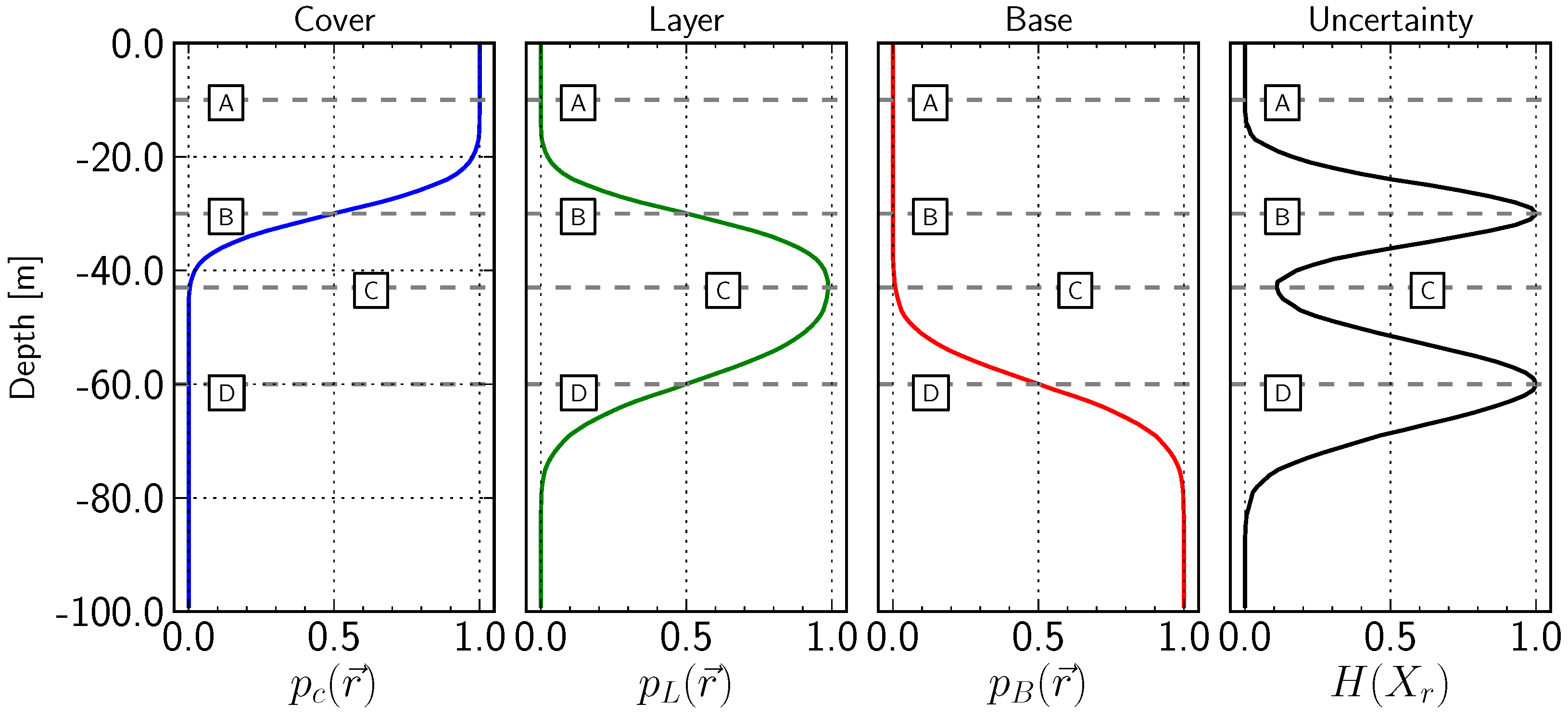
In the following, the focus will be on the analysis of uncertainties at this potential drill-hole location. The probabilities to obtain each of the geological units (the cover, the layer of interest, and the base layer) are derived from 1000 simulated model realisations. For the numerical analysis, the model is gridded to cell sizes of 10 m by 10 m . Results are shown in Figure 3. Please note that depth is downwards, as customary in representations of drill-hole data. The forth graph shows the information entropy H ( X r ) at each position r, calculated from the probabilities using Equation (4). Note that, in this case, only the z-value at position r = ( x , y , z ) changes.
Figure 3. Probability distribution of geological units ( p C ( r ) for the cover layer, p L ( r ) for the layer of interest and p B ( r ) for the base) at depth in drill-hole example, and the corresponding information entropy H ( X r ) ; the dashed gray lines and the labels indicate important positions in the graph: A: p C = 1 , H = 0 : no uncertainty; at B and D, H = 1, two outcomes equally probable ( p C = p L = 0.5 at B, p L = p B = 0.5 at D); C: minimum of uncertainty for layer; see text for further description.
Entropy 15 01464 g003
An interpretation of the information entropy graph is instructive to highlight the use of this quantity as a measure of uncertainty. Several key points are highlighted in Figure 3 with dashed lines and labels. At the depth of the dashed line (label A), only one outcome is possible: the “Cover” unit with a probability of p C ( r ) = 1 , and the corresponding information entropy at this depth is zero, meaning that no uncertainty exists. The information entropy reaches its maximum value for two possible outcomes ( H = 1 ) at the two lines with labels B and D, where two outcomes are equally probable ( p C = p L = 0.5 at B, p L = p B = 0.5 at D). In this case, these positions are equivalent to the expected values of the upper and lower boundary of the geological layer of interest. Both of these outcomes are as expected from the setup of the problem described above (Figure 2).
It is interesting to note, however, that the lowest uncertainty in the range of the layer of interest is not exactly between the expected positions of the top and lower boundary (which would be at 45 m ), but actually shallower, at around 43 m (label C in Figure 3). The reason for the shallower position is that, as shown above, the position of the lower boundary has a higher standard deviation and this leads to a relatively lower uncertainty closer to the top boundary. In this case, the position corresponds to the highest probability of the layer of interest (green graph); however, this is not necessarily the general case.

3.2. Uncertainty Correlation between Two Locations at Depth

After the analysis of uncertainties with information entropy at single locations, correlations of uncertainty between different positions are evaluated in the next step. In order to determine the correlations in detail, the joint probability tables for all outcomes are determined from the simulation results for all combinations of locations. From these tables, all relevant information theoretic measures can be calculated using Equations (5)–(12). What is evaluated here is, therefore, how gaining knowledge about one specific location in the subsurface is related to uncertainties at all other locations. The important aspect is that these analyses are performed on the basis of the joint probability table and that no specific outcome has to be assumed, as the uncertainty correlations are a part of the underlying model.
Two types of spatial correlations of uncertainties can be expected:
  • In each of the areas of highest uncertainty (label B and D in Figure 3), knowing the outcome at one point will necessarily reduce the uncertainty in the surrounding areas. This is due to the set-up of the example simulation (representing here, for example, geological expert knowledge) where the boundary position in the subsurface is simulated as normally distributed around an expected value.
  • Uncertain areas about the top and the base of the layer of interest should be correlated and knowing the outcome in the uncertain area about the top of the layer should influence uncertainties about the base, and vice versa. Although this correlation might be counter-intuitive, it follows from the set-up of the model with the top of the layer of interest defined, and the thickness considered uncertain (and not the base of the layer).
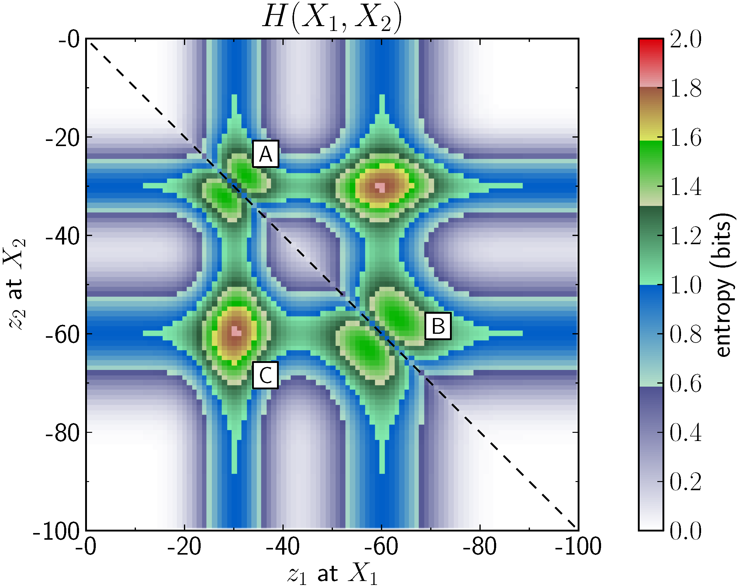
Each discrete cell in the model is considered as a separate random variable. In a first step, the joint and conditional entropy for all pair-wise combinations of all cells along the potential drill-hole location are evaluated. The results of the analysis are shown in Figure 4 and Figure 5. Each point in the visualised matrices corresponds to a pair of depth values ( z 1 at the location of the variable X 1 and z 2 at the position of the variable X 2 ). The colour bar in all of the following figures is set to highlight the log 2 step levels (for values > log 2 ( n ) , at least n + 1 (joint) outcomes are possible). Note that an additional step is included in every range to highlight changes within this step (e.g., between n = 1 and log 2 ( n = 2 ) = 1 at log 2 ( n = 1.5 ) 0.58 . As in the figures before, depth is represented from top to bottom on the y-axis. The representation of the joint entropy (Figure 4) reveals a pattern that is similar to the information entropy of one variable: it is high in the areas of uncertainty, in the range of the top of the layer at 25–35 m (label A) and near the base of the layer at around 55–65 m (label B). It is interesting to note that the joint entropy reaches its maximal value for position pairs between the top and the base layer (e.g., at label C).
The conditional entropy of a cell in the subsurface, represented as variable X 2 at a depth of z 2 , given the outcome of a variable X 1 at a depth z 1 is represented in Figure 5. The figure can be interpreted in a way that the vertical slice at a position z 1 corresponds to the remaining uncertainty depth profile (for all values z 2 ), given the information of variable X 1 at a depth z 1 . The conditional entropy highlights the same features that could be expected from the analysis of the joint entropy: the high uncertainties around the top and the base of the layer are reduced when spatially close outcomes are known (labels A and B), and, additionally, the uncertainties around the base of the layer are reduced when areas near the top are known (label C), and vice versa (label D). However, the important distinction is that conditional entropy can directly be interpreted as a reduction of uncertainty, and that the value at each location is lower or equal to the initial information entropy (Equation (9)). This important feature will be evaluated in more detail below. For comparison, the plot on the right in Figure 5 shows the values of information entropy at depth. It is equivalent to the plot in Figure 3. An important additional aspect of the conditional entropy is also highlighted in the figure: as opposed to the joint entropy, conditional entropy is not a symmetrical measure, H ( X 2 | X 1 ) H ( X 1 | X 2 ) .
Figure 4. Joint entropy between two variables at different z-values (depth in drill-hole). Labels correspond to important features, explained in detail in the text. The colour bar is set to reflect increments of log 2 ( n ) , with an additional subdivision between two steps for visualisation purposes. Joint entropy is a symmetrical measure, the dashed line represents z 1 = z 2 .
Entropy 15 01464 g004
In addition to the evaluation of uncertainty reduction, an important aspect of spatial uncertainty estimation is to determine how uncertainties are correlated, or which locations share information about uncertainties in space. The joint entropy in Figure 4 provides an indication of correlation; however, it is strongly dependent on the information entropy in each of the considered cells and therefore difficult to interpret. It has, for example, the disadvantage that pairs that certainly do not share any information, for example cases where the information entropy of one value is zero, can still be greater than zero (see, for example, the (0,60) pair, etc.).
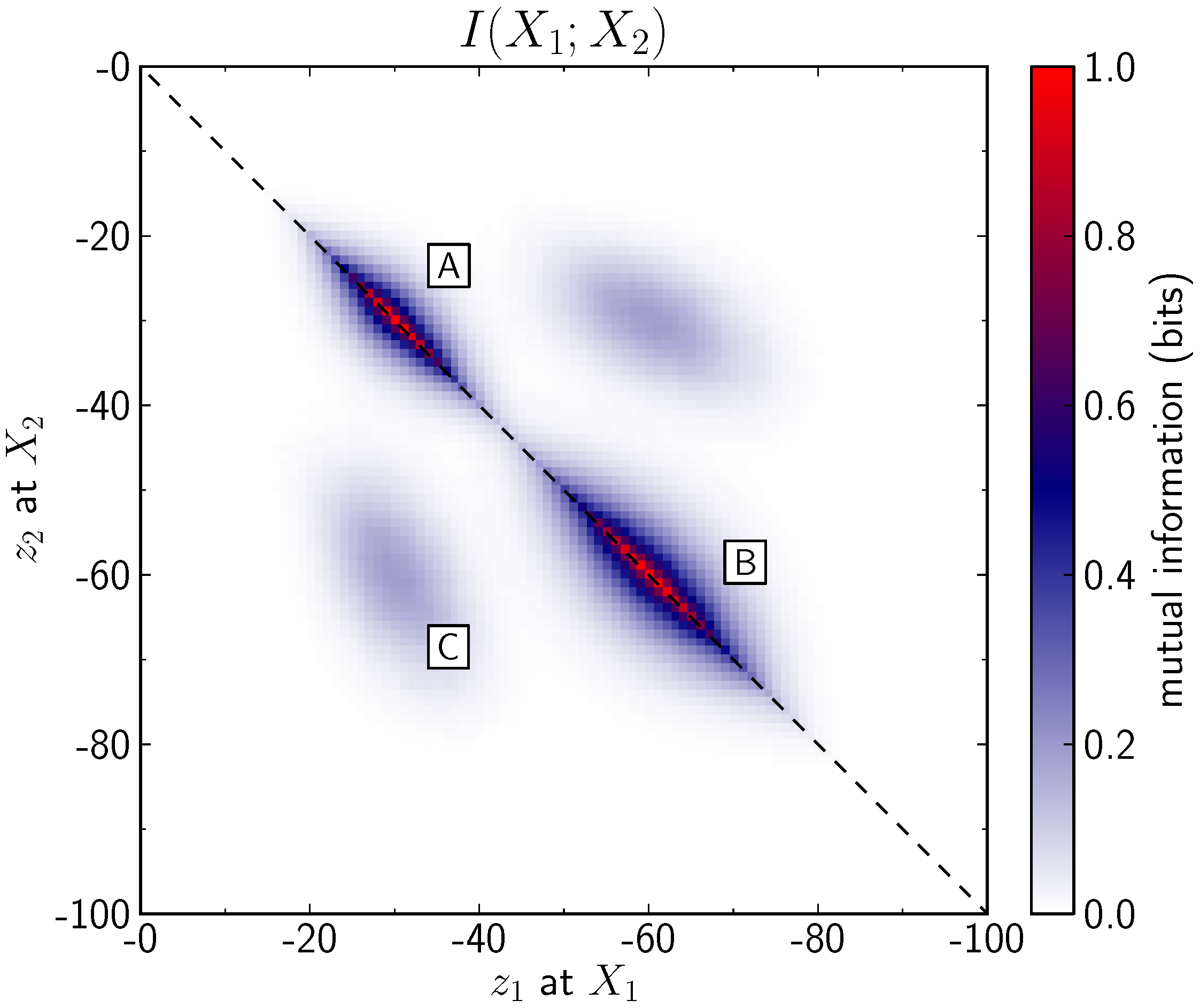
A more suitable measure for the interpretation of uncertainty correlations is mutual information. From Equation (12) it is apparent that it takes into account the information entropy of both variables, reduced by the joint entropy between them. An evaluation of the mutual information between all pairs of variables in the drill-hole example is shown in Figure 6. All the expected correlations are here clearly visible. The highest amount of shared information exists in cells close to each other, in the uncertain areas about the top (label A) and the base (label B) of the layer. In addition, the correlation between cells around the top and the base of the layer are apparent (label C), although clearly those correlations are weaker than the correlations at labels A and B. The figure also shows the symmetric nature of the mutual information.
Figure 5. Conditional entropy of one variable X 2 at depth, given the information of another variable X 1 . It is interesting to note that the entropies around z 2 = 60 m are reduced when information around a depth of z 1 = 30 m is obtained (label C) and vice versa (label D). The figure also clearly shows that conditional entropy is not symmetrical. The colour bar is set to reflect increments of log 2 ( 0.5 ) .
Entropy 15 01464 g005
Figure 6. Mutual information between two random variables X 1 and X 2 at different z-positions in the drill-hole example. Variables close to each other with high entropy share a large amount of information (labels A and B). However, it is also interesting to note that variables at locations close to the top share information with variables around the base of the layer (label C). Mutual information is a symmetrical measure, the dashed line represents the symmetry axis, z 1 = z 2 .
Entropy 15 01464 g006

3.3. Interpretation of the Relationship between all Measures

The examples before showed how the different measures from information theory provide insights into a variety of aspects of uncertainties and their spatial correlation in the subsurface. However, the relationships between the measures can be difficult to interpret. For clarification, two examples will be evaluated in more detail.
In the example of uncertainties in the drill-hole, it was shown that the joint entropy between a locations of z 1 = 30 m and z 2 = 60 m (Label C in Figure 4) was higher than the joint entropy between close points, for example between z 1 = 30 m and z 2 = 31 m , whereas the mutual information behaves in the opposite way. This important difference is due to the information entropy of each variable by itself. For a visualisation of the relationships, all pair-wise information theoretic measures for those cases are represented in the diagrams in Figure 7.
Figure 7. Graphical representation of the relationships between information entropy, joint entropy, conditional entropy, and mutual information (after [17]). The z values correspond to the actual depth values in the drill-hole example and the corresponding pair-wise entropy measures, see Figure 4, Figure 5 and Figure 6. (a) X 1 at z 1 = 30 m , X 2 at z 2 = 31 m ; (b) X 1 at z 1 = 30 m , X 2 at z 2 = 60 m .
Entropy 15 01464 g007
In the diagrams, the interpretation of joint entropy is clearly visible: the information entropy of each outcome by itself ( H ( X 1 ) and H ( X 2 ) ) is approximately the same in both cases. However, in the case of the close points in Figure 7a, both points share more information, reflected in a higher mutual information I ( X 1 ; X 2 ) , than in the case of the points that are further separated (Figure 7b). Also, the joint entropy is small for the former case, as well as the conditional entropies, H ( X 2 | X 1 ) and H ( X 1 | X 2 ) . Therefore, gaining information at z = 30 m will lead to a higher reduction of uncertainty in the surrounding cells, at the top of the layer, than in the cells around the base of the layer that are further away, exactly as it would intuitively be expected in this setting.

3.4. Application of Multivariate Conditional Entropy to Determine Entropy Reduction during Drilling

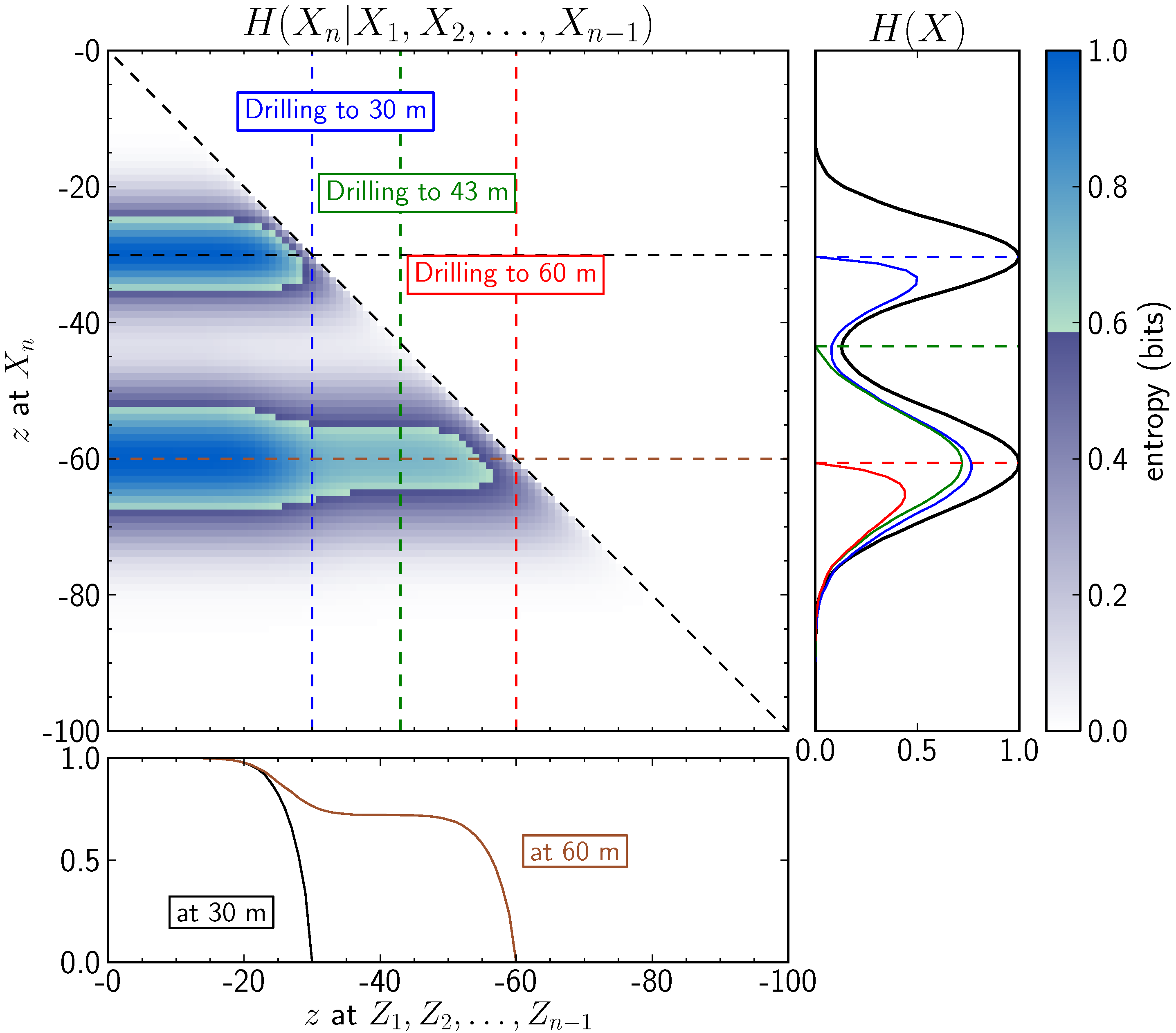
The interpretation of uncertainties in the pair-wise comparison shown before provided an insight into the correlation between two locations. The analysis has successfully highlighted the fact that uncertainties about the top surface of the layer are correlated with uncertainties of the base. In a practical sense, however, it is often of interest to consider the overall reduction of uncertainty when the values at multiple locations are known. As an example, in the case of the drill-hole application before, if we were to actually drill at this location, we would obtain information along the entire drill path, and not only at the deepest location. As the entropies along the path can be expected to be correlated (as shown in this case in Figure 6), the sum of the conditional entropies provides only an upper bound and would therefore lead to an underestimation of the remaining uncertainties. The correct measure to determine the remaining entropies is the multivariate conditional entropy (Equation (17)) of each cell in the model space, given the information of all cells along the drill path. The results are presented in Figure 8. In essence, the matrix visualisation is comparable with the pairwise conditional entropy plot in Figure 5. However, values in y-direction now represent the remaining uncertainties at a depth z, given the information of all variables X 1 , X 2 , , X n 1 at shallower depths z 1 , z 2 , , z n 1 . According to the definition of conditional entropy, values along a horizontal slice therefore have to decrease monotonically, reflecting the fact that uncertainties can only be reduced when new information is gained. This behaviour is shown for conditional entropies at the locations of highest uncertainty, at 30 m and 60 m , in the subfigure at the bottom in Figure 8. After the drill path reached the cell, the remaining uncertainty at this location is, as expected, reduced to zero.
Figure 8. Reduction of conditional entropy during information gain; the matrix visualisation is comparable with Figure 5 but shows here the remaining uncertainty of a variable X n at a position z n , given the information of all variables X 1 , X 2 , , X n 1 at shallower positions z 1 , z 2 , , z n 1 ; the bottom figure shows cuts in x-direction through the matrix, at the positions of highest uncertainty (30 m and 60 m ); the right figure shows conditional entropy profiles with remaining uncertainties after drilling to 30 m , 43 m , and 60 m .
Entropy 15 01464 g008
The subfigure on the right of Figure 8 shows conditional entropy profiles of remaining uncertainties, given a drilling to a specific depth. In addition, the black line shows the model information entropy, as the initial state of uncertainty. It is clearly visible that, after drilling to a depth to 30 m (blue line), uncertainties are reduced not only about the top surface of the layer but also about the base of the layer (at around 60 m ). Further drilling to the expected centre of the layer at around 43 m (green line) does not reduce uncertainty significantly more. The red line, finally, shows the remaining uncertainties that can be expected after drilling to the expected base of the layer, at 60 m .
This example clearly shows how information theoretic measure can be used not only to quantify uncertainties at specific locations at depth but also to evaluate how uncertainties—and information—are correlated in space. Making use of this estimation of correlation, it is then possible to determine how gaining information in one part of the model will reduce uncertainties in other areas.

3.5. Determination of Structural Correlations of Uncertainty in a Higher Dimension

In the previous example, we considered uncertainties for the 1-D case at a potential drilling location. The logical extension of this example is to consider the uncertainty reduction not only along this drill-hole, but also in areas further away from the drilling location. In order to evaluate the application of the information theoretic measures in this context, the previous conceptual geological model is extended into higher dimensions. The uncertainty correlations in a typical geological structure, i.e., a fold, will be evaluated. In a simplified conceptual form, a fold can be considered as a sinusoidal layer that is formed due to the compression of a stiff layer in a soft matrix, for example as a result of a compressional tectonic event. For the case of gentle folding, the structure can be assumed to be strictly symmetric. As in the one-dimensional case before, prior geological knowledge about the structure of the folding might exist, for example from comparison with field observations, and geological assumptions.
Four additional parameters are introduced to simulate the effect of the folded layer: the fold amplitude, defined by a normal distribution with a mean of 3 m and a standard deviation of 3 m , and the fold period, with a mean period of 80 m and a standard deviation of 5 m . In addition, the lateral position of the fold is randomly changed (see Figure 9).
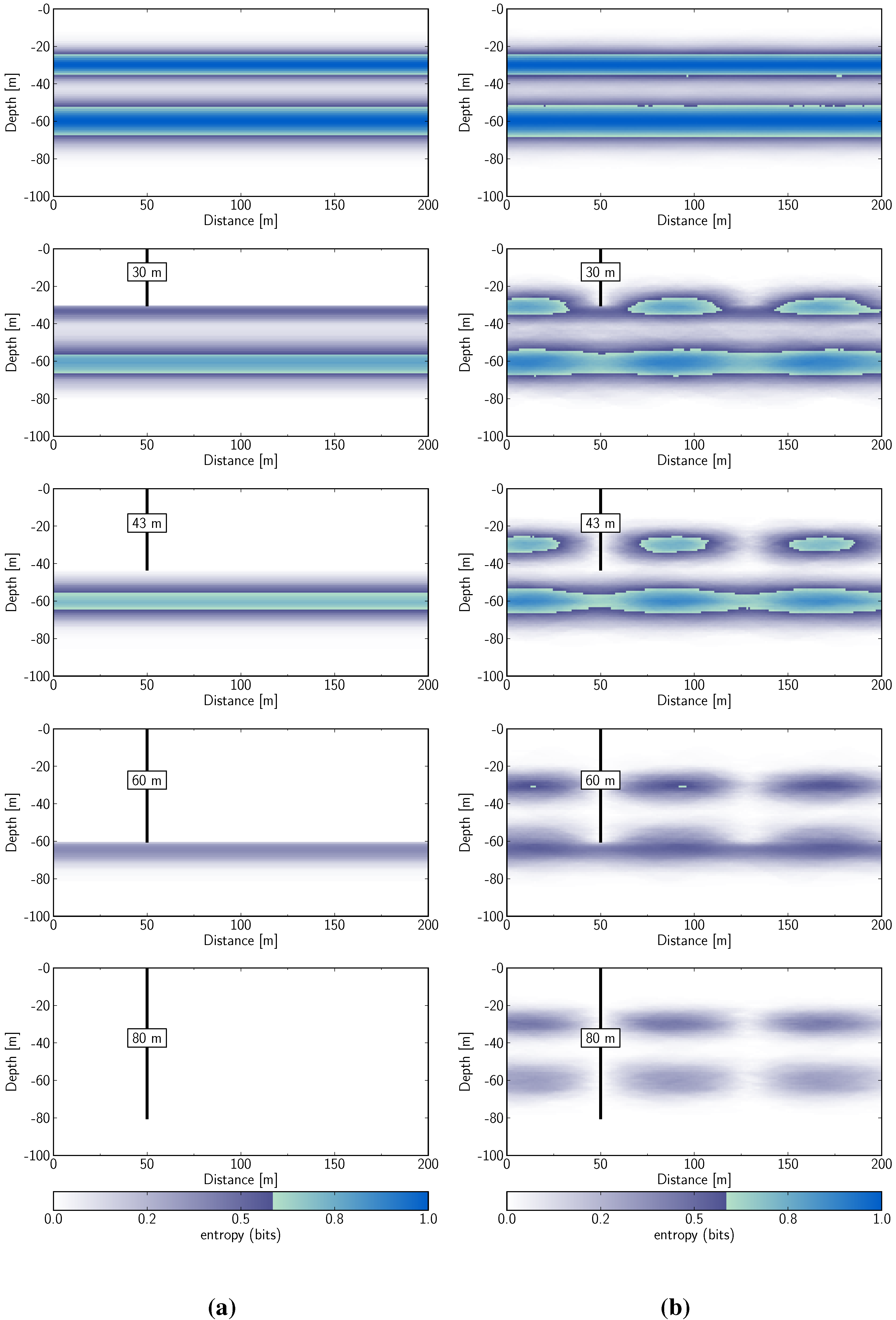
We will now compare the spatial reduction of uncertainty for both geological scenarios, the example of the planar surface of Figure 2, essentially equivalent to the 1-D case studied above, and the case of the additional folding, represented in Figure 9. As before, a total of 1000 models were randomly generated for each scenario with a cell resolution of 10 m . Probability fields for each possible outcome were estimated from the simulated realisations. Results of this analysis are presented in the top row of Figure 10. The left column corresponds to the model with the planar surface (Figure 10a), and the right column to the model with a potential sinusoidal surface (Figure 10b). Please note that these figures now actually represent vertical cross-sections in space, with depth along the y-axis, and distance along the x-axis, as opposed to the pair-wise location comparison in Figure 4, Figure 5 and Figure 6. The first row of figures represents the information entropy (Equation (1)) for both scenarios. The information entropy is almost identical for both cases, with remaining differences due to the shape of the sine function, and numerical noise.
Figure 9. Extension of the example model to simulate folded top and base surfaces of the central layer.
Entropy 15 01464 g009
The following rows in Figure 10a represent the multivariate conditional entropy of each location in the model, given the combined information of all cells that are part of the drill-hole, calculated with Equation (18). These figures can be interpreted as the uncertainty reduction that can be expected with the information gained during drilling (here at an arbitrary location at 50 m ). The spatial characteristics of uncertainty reduction for the case of the planar surface in Figure 10a is a lateral extrusion of the 1-D example, analysed in detail in Figure 8, with corresponding steps of “drilling depth” (directly comparable with the curves in the right subfigure of Figure 8). As expected, as soon as we reach a specific drilling depth, uncertainties above this depth are reduced to zero. As soon as the drilling depth extends below a position where the lower boundary can reasonably be expected (at 80 m ), everything has to be known and there are no remaining uncertainties.
The characteristics of uncertainty reduction are different for the case of the potential sinusoidal surface, shown in Figure 10b. The first obvious difference is the fact that clear lateral variations of uncertainty reduction exist. In the case of the drilling to 30 m , significant uncertainties remain at a lateral distance of approximately 40 m from the drill-hole location. However, the conditional entropy also shows that the uncertainty is then reduced again at a distance of approximately 80 m . Both aspects nicely reflect the sinusoidal lateral variation used as an input for the simulation (Figure 9). Drilling to the depth with the highest probability of the layer, at around 43 m , leads only to a small further uncertainty reduction. However, drilling to 60 m , around the depth of the expected base of the layer, clearly reduces uncertainties about the base. Another interesting observation is that drilling to the base of the layer also reduces the remaining uncertainties around top surface even further. Finally, even after drilling through the entire depth of the potential layer, uncertainties remain in the sinusoidal model, as shown in the bottom of Figure 10b. The multivariate conditional entropy clearly highlights the differences in uncertainty and their spatial correlation between the restricted case of planar surfaces, where all uncertainties would be completely resolved, and the additional lateral uncertainty added by the potential folding of the layer.
Figure 10. Spatial distribution of conditional entropy, indicating uncertainty reduction during drilling. (a) Planar surfaces (Figure 2); (b) Folded surfaces (Figure 9).
Entropy 15 01464 g010
The study highlighted the application of measures from information theory to evaluate different aspects of spatial uncertainty: the analysis and quantification of uncertainties in space, the evaluation of uncertainty correlations between two locations, and finally the analysis of how additional information could be expected to reduce uncertainties in space. The most relevant aspects are summarised in Table 1. The different measures are assigned to important “steps” in the analysis as used in the evaluation before. In a different context, only a subset of these analyses might be performed. Step I identifies the initial part of an uncertainty study: the quantification and visualisation of uncertainties in space. The information entropy of one variable has been applied previously to visualise and quantify spatial uncertainties [1,2,14], and joint entropy is the logical extension to two variables. Step II addresses the question of uncertainty correlation and analyses how much information two variables, or in the spatial context, two locations, share. It is also directly evident from the representation of the relationships between the measures in Figure 7 that for cases where two variables share no information, having the information at one location will not reduce uncertainties at the other location. The uncertainty reduction itself is performed with the measures of conditional entropy, step III in Table 1. The important aspect of conditional entropy is that it provides a direct estimation of the remaining uncertainty at one location, given additional data at one or more (for the multivariate case) other locations in space. To close the loop, this remaining uncertainty estimate is directly comparable with the initial uncertainty, estimated with information entropy in step I. All measures combined provide consequently a coherent framework for the analysis and quantification of spatial uncertainties, their correlation, and potential reductions of uncertainties with additional information.
Table 1. Application of information theoretic measures for uncertainty estimation, correlation analysis, and estimations of uncertainty reduction.
StepMeasureUseVariablesSpatial Interpretation
IInformation entropyUncertainty quantificationSingle variableAnalysis of uncertainty at one location
Joint entropyUncertainty quantificationTwo variablesAnalysis of combined uncertainty at two locations
IIMutual informationCorrelation analysisTwo variablesEstimate of information shared between two different locations in space
IIIConditional entropyUncertainty reductionTwo variablesEstimate of how information at one location would reduce uncertainty in space
Multivariate conditional entropyUncertainty reductionMultiple variablesEstimate of how information at multiple locations would reduce uncertainty in space

4. Discussion and Conclusions

The application of the information theoretic measures of joint entropy, conditional entropy, and mutual information evidently confirm the hypothesis that the measures provide a detailed insight into correlations and reductions of uncertainty in a spatial context. Based on the initial application of information entropy to determine uncertainties in space, mutual information and conditional entropy represent the complementary measures to interpret correlations and expected reductions of uncertainties. A detailed comparison of all measures to a typical geological uncertainty scenario showed that mutual information can be used to determine which locations in a model are correlated and share information in the context of uncertainties. Conditional entropy can then be used to calculate how much uncertainty would remain at one location, given information at another location. Detailed examination of expected uncertainty reduction during subsequent information gain, for example along the path of a drilling, showed that multivariate conditional entropy provides a measure for one of the most important aspects in the context of spatial uncertainty, i.e., the evaluation of where information will be most useful to reduce uncertainties in space. Or, to put it plainly in the context of exploration: where to drill next?
A meaningful interpretation of spatial uncertainties, correlations, and potential reductions of uncertainty clearly depends on the characteristics of the underlying probability fields. If these probability fields are derived from model simulations, as in the example shown before, then the analysis relies on the use of an appropriate model. The comparison of the planar structure with the gently folded layer showed how alternative assumptions about the geological setting lead to different estimations of uncertainty reduction (Figure 10). As an alternative interpretation, should prior knowledge exist that the surface is planar rather than folded, then it could be expected that uncertainties are completely reduced after drilling at one location. The information theoretic measures enable this evaluation of spatial uncertainties because the analysis itself is not based on any assumptions of spatial dependencies (as opposed to analyses using variograms, for example). All correlations of uncertainty that are determined in the analysis are directly related to the underlying model. In the examples before, these correlations were evident from the parameterisation of the problem. However, in more complex cases, this is an important aspect for the determination of correlations due to multiple interacting uncertainties that are not directly obvious from the model definition itself.
In recent years, new approaches have been developed to create multiple realisations for uncertainty estimations in complex three-dimensional structural geological models (e.g., [12,13,20,23,24,26,27,28,29]). It is expected that an application of information theoretic measures to these more complex settings will reveal novel and valuable insights into uncertainties and their potential reduction in realistic research and exploration scenarios. In addition, the methods can be applied to the analysis of uncertainties under the consideration of expected structures in a variety of other research areas, for example in the analysis of tomographic data in medical and material sciences where the shape of an expected structure might be known, but the exact position uncertain.
In addition to the spatial analysis of uncertainties presented above, it is important to note that information theory provides a way forward to analyse uncertainties on the scale of the system. This possibility has been applied before in the context of structural geological models using information entropy [2]. An extension of this concept, utilising the uncertainty correlation measures described above, will open up the way for a detailed analysis of the state of uncertainty in a geological system, an important aspect in a wide range of geological applications, and an exciting path for future work.
In summary, information theoretic measures provide an ideal framework for a consistent analysis of spatial uncertainty, correlations of uncertainty between different locations, and estimates of uncertainty reduction with additional information in all cases where spatial uncertainties are relevant in maps and models.

Acknowledgements

The author is funded by a CSIRO Office of the Chief Executive Post-Doctoral Fellowship scheme within the CSIRO Earth Science and Resource Engineering Division. The manuscript benefitted greatly from stimulating discussions with Jürg Hauser and Klaus Regenauer-Lieb and the helpful comments of two anonymous reviewers.

Appendix

A. Information Entropy of a Coin Flip

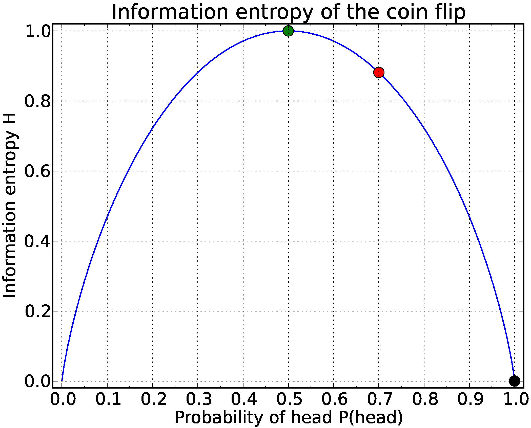
The typical coin flip is a good example to explain the important aspects of information entropy in relation to the probabilities of an outcome.
Figure A1. Information entropy of a binary system: in the case of the fair coin with P(head) = P(tail) = 0.5, the information entropy is maximal with a value of H ( 0.5 ) = 1 (green dot); in the case of the bent coin with P(head) = 0.7, the uncertainty of the system is reduced, and the information entropy is accordingly lower H ( 0.7 ) 0.88 (red dot). In the case of a double headed coin with P(head) = 1, no uncertainty remains because the outcome is known, and H ( 1.0 ) = 0 (black dot).
Entropy 15 01464 g011
If the coin is fair, then the probability of each outcome is p ( head ) = p ( tail ) = 0.5 . According to Equation (3), the entropy of this two outcome system therefore has its maximum value. Using Equation (1), this value is H ( coin ) = 0.5 · log 2 0.5 0.5 · log 2 0.5 = 1 . Let us now assume that we managed to obtain a coin that has a higher chance of obtaining head, for example with p ( head ) = 0.7 (imagine, for example, a bent coin). In this case, the information entropy of the coin flip experiment would be H ( unfaircoin ) = 0.7 · log 2 0.7 0.3 · log 2 0.3 0.88 . The uncertainty of the experiment is lower because one outcome is more probable. In the extreme case of a double-headed coin, the probability of head would be 1 and the information entropy of the coin flip would be 0, corresponding to the fact that no uncertainty exists because the outcome of the experiment is already known. For more details on the interpretation see, for example, the excellence descriptions in Ben-Naim [17] or MacKay [16].

References

  1. Potter, K.; Gerber, S.; Anderson, E.W. Visualization of uncertainty without a mean. IEEE Comput. Graph. Appl. 2013, 33, 75–79. [Google Scholar] [CrossRef] [PubMed]
  2. Wellmann, J.F.; Regenauer-Lieb, K. Uncertainties have a meaning: Information entropy as a quality measure for 3-D geological models. Tectonophysics 2012, 526–529, 207–216. [Google Scholar] [CrossRef]
  3. Zhang, J.; Goodchild, M.F. Uncertainty in Geographical Information; Taylor & Francis: New York, NY, USA, 2002. [Google Scholar]
  4. Devillers, R.; Jeansoulin, R. Fundamentals of Spatial Data Quality; ISTE: London, UK, 2006. [Google Scholar]
  5. Atkinson, P.M.; Foody, G.M. Uncertainty in remote sensing and GIS: Fundamentals. In Uncertainty in Remote Sensing and GIS; John Wiley & Sons, Ltd: Chichester, UK, 2006; pp. 1–18. [Google Scholar]
  6. Jeansoulin, R.; Papini, O.; Prade, H.; Schockaert, S. Introduction: Uncertainty issues in spatial information. In Studies in Fuzziness and Soft Computing; Jeansoulin, R., Papini, O., Prade, H., Schockaert, S., Eds.; Springer: Heidelberg, Germany, 2010; pp. 1–11. [Google Scholar]
  7. Fisher, P.; Comber, A.; Wadsworth, R. Approaches to Uncertainty in Spatial Data. In Fundamentals of Spatial Data Quality; ISTE: London, UK, 2006; pp. 43–59. [Google Scholar]
  8. Chilès, J.P.; Delfiner, P. Geostatistics: Modeling Spatial Uncertainty; Wiley: New York, NY, USA, 1999. [Google Scholar]
  9. Deutsch, V.C. Geostatistical Reservoir Modeling (Applied Geostatistics Series); Oxford University Press: New York, NY, USA, 2002. [Google Scholar]
  10. Turner, A. Challenges and trends for geological modelling and visualisation. Bull. Eng. Geol. Environ. 2006, 65, 109–127. [Google Scholar] [CrossRef]
  11. Caers, J. Modeling Uncertainty in the Earth Sciences; John Wiley & Sons, Ltd: Chichester, UK, 2011. [Google Scholar]
  12. Wellmann, J.F.; Horowitz, F.G.; Schill, E.; Regenauer-Lieb, K. Towards incorporating uncertainty of structural data in 3D geological inversion. Tectonophysics 2010, 490, 141–151. [Google Scholar] [CrossRef]
  13. Lindsay, M.; Aillères, L.; Jessell, M.; de Kemp, E.; Betts, P.G. Locating and quantifying geological uncertainty in three-dimensional models: Analysis of the Gippsland Basin, southeastern Australia. Tectonophysics 2012, 546–547, 1–44. [Google Scholar] [CrossRef]
  14. Goodchild, F.M.; Buttenfield, B.; Wood, J. Introduction to visualizing data validity. In Visualization in Geographical Information Systems; Hearnshaw, M.H., Unwin, J.D., Eds.; John Wiley & Sons: New York, NY, USA, 1994; pp. 141–149. [Google Scholar]
  15. Cover, T.M.; Thomas, J.A. Elements of Information Theory, 2nd ed.; John Wiley & Sons, Inc.: Hoboken, NJ, USA, 2005. [Google Scholar]
  16. MacKay, D.J. Information Theory, Inference, and Learning Algorithms, 4th ed.; Cambridge University Press: Cambridge, UK, 2003. [Google Scholar]
  17. Ben-Naim, A. A Farewell to Entropy; World Scientific: Singapore, 2008. [Google Scholar]
  18. Shannon, E.C. A mathematical theory of communication. Bell Syst. Tech. J. 1948, 27, 379–423. [Google Scholar] [CrossRef]
  19. Metropolis, N.; Ulam, S. The monte carlo method. J. Am. Stat. Assoc. 1949, 44, 335–341. [Google Scholar] [CrossRef] [PubMed]
  20. Tacher, L.; Pomian-Srzednicki, I.; Parriaux, A. Geological uncertainties associated with 3-D subsurface models. Comput. Geosci. 2006, 32, 212–221. [Google Scholar] [CrossRef]
  21. Thore, P.; Shtuka, A.; Lecour, M.; Ait-Ettajer, T.; Cognot, R. Structural uncertainties: Determination, management, and applications. Geophysics 2002, 67, 840–852. [Google Scholar] [CrossRef]
  22. Bardossy, G.; Fodor, J. Evaluation of Uncertainties and Risks in Geology: New Mathematical Approaches for their Handling; Springer: Berlin, Germany, 2004. [Google Scholar]
  23. Suzuki, S.; Caumon, G.; Caers, J. Dynamic data integration for structural modeling: Model screening approach using a distance-based model parameterization. Comput. Geosci. 2008, 12, 105–119. [Google Scholar] [CrossRef]
  24. Lindsay, M.; Aillères, L.; Jessell, M. Integrating geological uncertainty into combined geological and potential field inversions. In Proceedings of the GeoMod 2010 Conference, Lisbon, Portugal, 27–29 September 2010.
  25. Refsgaard, C.J.; Christensen, S.; Sonnenborg, O.T.; Seifert, D.; Højberg, L.A.; Troldborg, L. Review of strategies for handling geological uncertainty in groundwater flow and transport modelling. Adv. Water Resour. 2011, 36, 36–50. [Google Scholar] [CrossRef]
  26. Bistacchi, A.; Massironi, M.; Dal Piaz, V.G.; Monopoli, B.; Schiavo, A.; Toffolon, G. 3D fold and fault reconstruction with an uncertainty model: An example from an Alpine tunnel case study. Comput. Geosci. 2008, 34, 351–372. [Google Scholar] [CrossRef]
  27. Cherpeau, N.; Caumon, G.; Lévy, B. Stochastic simulations of fault networks in 3D structural modeling. Compt. Rendus Geosci. 2010, 342, 687–694. [Google Scholar] [CrossRef]
  28. Judge, P.A.; Allmendinger, R.W. Assessing uncertainties in balanced cross sections. J. Struct. Geol. 2011, 33, 458–467. [Google Scholar] [CrossRef]
  29. Cherpeau, N.; Caumon, G.; Caers, J.; Lévy, B. Method for stochastic inverse modeling of fault geometry and connectivity using flow data. Math. Geosci. 2012, 44, 147–168. [Google Scholar] [CrossRef]