Article

Information Properties of Boundary Line Models for N2O Emissions from Agricultural Soils

1
Crop and Soil Systems, SRUC, West Mains Road, Edinburgh, EH9 3JG, UK
2
Division of Science Delivery, Department of Science, Information Technology, Innovation and the Arts, GPO Box 5078, Brisbane, QLD 4001, Australia
3
Carbon Management Centre, SRUC, West Mains Road, Edinburgh EH9 3JG, UK
*
Authors to whom correspondence should be addressed.
Entropy 2013, 15(3), 972-987; https://doi.org/10.3390/e15030972
Submission received: 15 January 2013 / Revised: 25 February 2013 / Accepted: 27 February 2013 / Published: 5 March 2013
(This article belongs to the Special Issue Applications of Information Theory in the Geosciences)

Abstract

:
Boundary line models for N2O emissions from agricultural soils provide a means of estimating emissions within defined ranges. Boundary line models partition a two-dimensional region of parameter space into sub-regions by means of thresholds based on relationships between N2O emissions and explanatory variables, typically using soil data available from laboratory or field studies. Such models are intermediate in complexity between the use of IPCC emission factors and complex process-based models. Model calibration involves characterizing the extent to which observed data are correctly forecast. Writing the numerical results from graphical two-threshold boundary line models as 3×3 prediction-realization tables facilitates calculation of expected mutual information, a measure of the amount of information about the observations contained in the forecasts. Whereas mutual information characterizes the performance of a forecaster averaged over all forecast categories, specific information and relative entropy both characterize aspects of the amount of information contained in particular forecasts. We calculate and interpret these information quantities for experimental N2O emissions data.

1. Introduction

Over the last few decades, the atmospheric concentration of nitrous oxide (N2O) has been increasing. Agricultural soils are a significant source of N2O emissions [1]. Under the Kyoto Protocol, over 170 nations agreed to develop national inventories of anthropogenic emissions. These are calculated using the IPCC emission factors [2], which assume that the annual N2O emissions from agricultural soils are proportional to the N applied, and which are mostly based on emission factors developed by Bouwman [3]. This is the simplest approach to calculating emissions.
However, the rate of N2O emissions is affected by soil characteristics and climate [4,5,6,7,8], soil management [1,4,9] and the crops planted [4,10,11]. Thus, in order to incorporate these factors into estimates of N2O emissions, more complex process-based models have been developed. These include DAYCENT [12] and DNDC [13,14]. Although it is recognized that they have the ability to test different management and mitigation options, these models require large amounts of input data and need to be calibrated for different agricultural systems.
The use of empirical models provides an approach to estimating N2O emissions intermediate in complexity between the IPCC emission factor approach and process-based models [15]. The idea is to use soil and climate data to estimate the corresponding level of N2O emissions [15]. Conen et al. [15] and Wang and Dalal [16] have used a boundary line model approach, based on water filled pore space, soil temperature and soil mineral N, to determine levels of N2O emissions from agricultural soils. Calibration for different agricultural systems is still required, but acquisition of the relevant input data is simpler than for process-based models.
In writing for this special issue of Entropy on Applications of Information Theory in the Geosciences, our emphasis is on practical applications. That is to say, we are interested in applications that relate to the analysis of models and observed data, and we are writing for colleagues in the experimental geosciences who, it is to be hoped, are attracted to this special issue by the prospect of finding, then assimilating and utilizing such applications. In particular, we will use an information theoretic analysis to address the properties of boundary line model forecasts of N2O emissions from agricultural soils.

2. Models and Data

2.1. Boundary Line Models
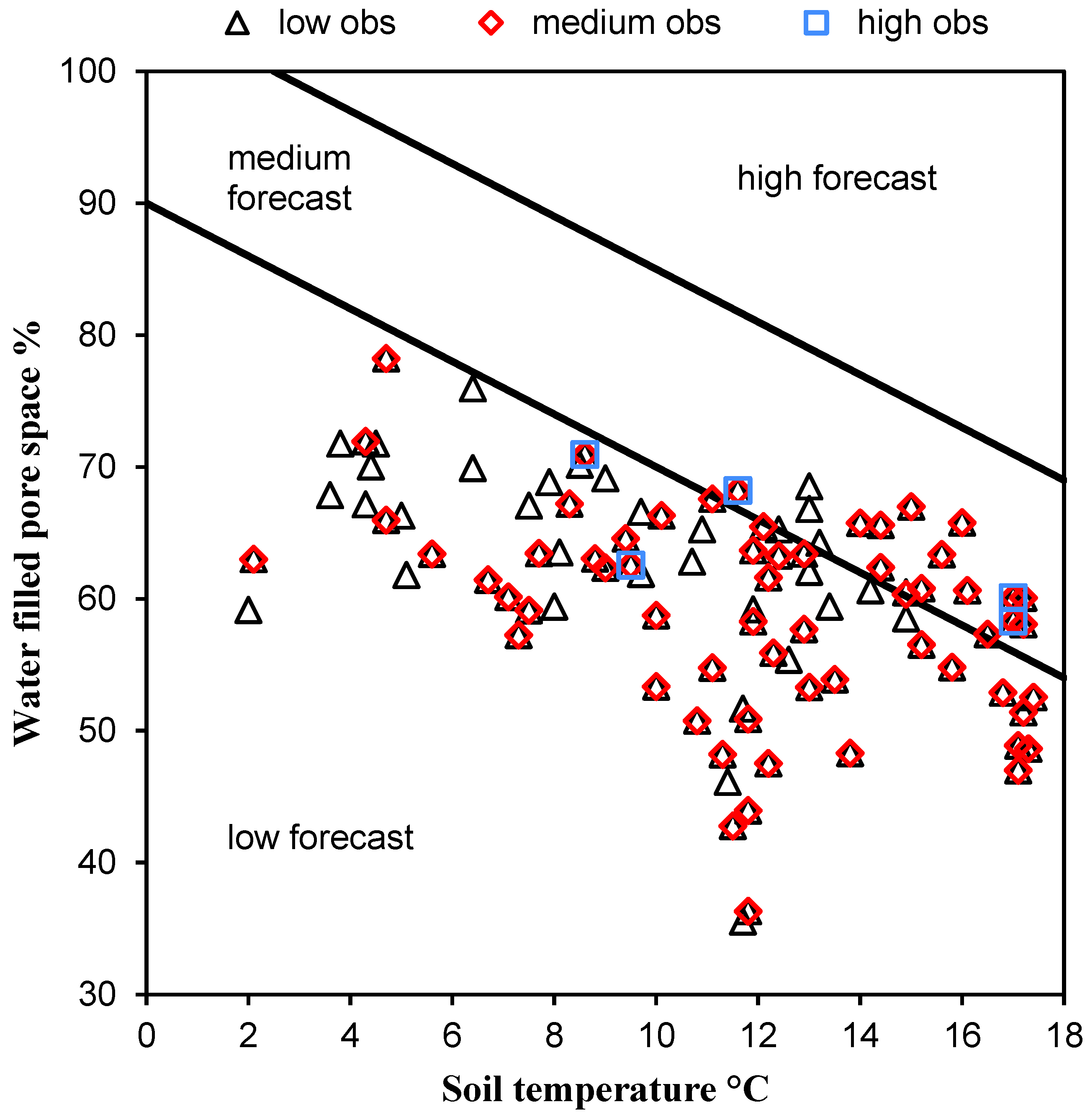
The response variable of interest here is N2O emission (or ‘flux’, g N2O-N ha−1 day−1). For the kind of boundary line model under consideration here, a two-dimensional region of parameter space is delimited by appropriate ranges (considering the observed data) of two continuous explanatory variables, soil water-filled pore space (WFPS, %) and soil temperature (T, °C). The parameter space is partitioned into sub-regions by means of thresholds based on relationships between N2O flux and the explanatory variables; two such thresholds partition the parameter space into three sub-regions of forecast N2O flux, denoted ‘low’, ‘medium’ and ‘high’.
For an introductory example, Figure 1 shows observed data from an intensive study of N2O emissions from sandy loam grassland soils at a site in Dumfries (SW Scotland) between March 2011 and March 2012, in which inorganic N fertilizer (ammonium nitrate and urea) treatments at a range of application rates (0, 80, 160, 240, 320, 400 kg/ha N) and additional 320 kg/ha N plus the nitrification inhibitor DCD were used. In Figure 1, the observed data are superimposed on the partitioned parameter space using the boundary lines for forecast N2O emissions as calculated in Conen et al. [15]. In this case, although the majority of the observed low emissions (<10 g N2O-N ha−1 day−1) were correctly forecast, only a minority of observed medium emissions (10-100 g N2O-N ha−1 day−1) and no observed high emissions (>100 g N2O-N ha−1 day−1) were correctly forecast. Here, these data serve only to make the point that it is important to be able to characterize the extent to which observed levels of N2O flux are correctly or incorrectly forecast by a boundary line model. Although these data are not analyzed further, we will discuss in Section 5 how other data sets present similar issues in terms of estimating N2O emissions from agricultural soils within defined ranges.
Figure 1. The parameter space delimited by observed ranges of water filled pore space (WFPS, %) and soil temperature (T, °C) in 2011-2012 at a grassland site in Dumfries, SW Scotland, receiving inorganic fertilizer, is the basis for a boundary line model. Observed N2O emissions were categorized as ‘low’ (<10 g N2O-N ha−1 day−1), ‘medium’ (10-100 g N2O-N ha−1 day−1) or ‘high’ (>100 g N2O-N ha−1 day−1), as in Conen et al. [15]. There were 715 ‘low’ observations, 322 ‘medium’ observations and 19 ‘high’ observations (N = 1056), resulting in many overlapping data points on the graph. The boundary lines between forecast emission categories are WFPS(%) + 2∙T(°C) = 90 (low-medium) and WFPS(%) + 2∙T(°C) = 105 (medium-high), as described in Conen et al. [15].
Entropy 15 00972 g001
At this stage, before discussing the details of any of the information quantities that may be used to analyze forecasts of N2O emissions, we note that the boundary line approach (as described in [15,16]) is intrinsically suitable for such analysis. For example, Tribus and McIrvine [17] note: “In modern information theory, probabilities are treated as a numerical encoding of a state of knowledge. One’s knowledge about a particular question can be represented by the assignment of a certain probability (denoted p) to the various conceivable answers to the question.” Thus the boundary line approach, as described, starts by characterizing the conceivable answers to the question of the magnitude of N2O flux (‘low’, ‘medium’ and ‘high’). Note that this specification restricts our attention to discrete distributions of probabilities.

2.2. Data

The data analyzed in this study come from an assessment of the boundary line approach for forecasting N2O emission ranges from Australian agricultural soils [16]. Observed emissions were categorized as ‘low’ (<16 g N2O-N ha−1 day−1), ‘medium’ (16-160 g N2O-N ha−1 day−1) or ‘high’ (>160 g N2O-N ha−1 day−1). Boundary lines were calculated separately for pasture and sugarcane soils (Table 1) and for cereal cropping soils (Table 2, see also Figure 2 in [16]). For a boundary line plot in which two thresholds partition the parameter space into three sub-regions of forecast N2O flux, denoted ‘low’, ‘medium’ and ‘high’, we can present the data in a 3×3 prediction-realization table in which the columns correspond to the observations, the rows to the forecasts. Theil [18] uses this terminology to refer both to the cross-tabulated frequencies of observations and forecasts, and to the estimated probabilities obtained by normalization of the frequencies. Here we present the normalized version of the data (Table 1 and Table 2, based on Figure 2 in [16]).
We adopt the following notation for Table 1 and subsequently. The observed categories are denoted oj (j=1,2,3) for ‘low’, ‘medium’ and ‘high’ N2O flux categories, respectively. The bottom row of the table contains the distribution Pr(O). The forecast categories are denoted fi (i=1,2,3) for ‘low’, ‘medium’ and ‘high’ N2O flux categories, respectively. The right-hand margin of the table contains the distribution Pr(F). The body of the table contains the joint probabilities Pr(ojfi). All values (here and throughout) are rounded to 4 d.p.
Table 1. Prediction-realization table based on N=271 observations of N2O flux for pasture and sugarcane soils from Figure 2 of [16]. The boundary lines between forecast emission categories were WFPS(%)+0.71∙T(°C) = 63 (low-medium) and WFPS(%)+0.71∙T(°C) = 75 (medium-high).
Forecast category, fiObserved category, ojRow sums
1. Low2. Medium3. High
1. Low0.28410.05540.00740.3469
2. Medium0.11810.15130.09590.3653
3. High0.04800.08120.15870.2878
Column sums0.45020.28780.26201.0000

3. Analysis of Information Properties

Shannon’s two papers, collected together as [19], represent the beginning of modern information theory; Cover and Thomas’s text [20] provides a comprehensive overview of half a century of progress. In the present context, where we are more concerned with applications of information theory relating to the analysis of models and data than with the mathematical theory of communications, readers may also find useful background in Attneave [21], Theil [18] or Hughes [22].

3.1. Information Content

We write p (=Pr(E), 0 ≤ Pr(E) ≤ 1) to denote a generic probability of an event E. Then h(p) = log(1/p) = −log(p) is the information content of a message that tells us, without error, that E has occurred (thus, in the present context, such a message constitutes a perfect forecast). If p is small, the information content of this message is large, and vice versa. If p=0 (the event is impossible) and you tell us that E has definitely occurred, the information content of this message is indefinitely large; if p=1 (the event is certain) and you tell us that E has definitely occurred, the information content of this message is zero. The base of the logarithm serves to define the units of information. In the mathematical theory of communications, logarithms base 2 are often used and the unit of information is the bit. Here we will use natural logarithms for calculations, and refer to the unit of information as the nit [23]. We will write log in places where the reference is generic.
Now consider the observed N2O flux categories o1 (‘low’), o2 (‘medium’) and o3 (‘high’), with corresponding probabilities Pr(o1), Pr(o2) and Pr(o3), j Pr ( o j ) = 1 , Pr ( o j ) 0 , j = 1 , 2 , 3. We cannot calculate the information content h ( Pr ( o j ) ) until the message is received, because the message ‘oj occurred’ may refer to any one of o1, o2 or o3. We can, however, calculate expected information content before the message is received. This quantity, often referred to as the entropy, is the weighted average of the information contents of the possible messages. Since the message ‘oj occurred’ is received with probability Pr(oj), the expected information content, denoted H(O), is:
H ( O ) = j Pr ( o j ) log ( Pr ( o j ) )
We note that H(O) ≥ 0 and take Pr(oj)log(Pr(oj)) = 0 if Pr(oj) = 0, since  lim  x 0 x log ( x ) = 0. If any Pr(oj) = 1, H(O) = 0. This is reasonable since we expect nothing from a forecast if we are already certain of the actual outcome. H(O) has its maximum value when all the Pr(oj) have the same value. This is also reasonable, since a message that tells us what actually happened will have a larger information content when all outcomes are equally probable than when some outcomes are more probable than others. Providing an everyday-language metaphor by means of which to characterize entropy is no easy task. Tribus and McIrvine [17] give a brief account of Shannon’s own difficulty in this respect. In the present context, entropy can be thought of as characterizing either information or uncertainty, depending on our point of view. At the outset, we know that just one of a number of events will occur, and the corresponding probabilities of the events. Entropy quantifies how much information we will obtain, on average, from a message that tells us what actually happened. Alternatively, entropy characterizes the extent of our uncertainty prior to receipt of the message that tells us what happened.
Now, similarly, we can calculate the entropy of the distribution of forecast N2O flux probabilities:
H ( F ) = i Pr ( f i ) log ( Pr ( f i ) )
and the entropy of the joint probability distribution:
H ( O , F ) = i j Pr ( o j f i ) log ( Pr ( o j f i ) )
Working in natural logarithms, we calculate from Table 1 [using Equations (1), (2) and (3), respectively] the expected information contents in nits as follows: H(O) = 1.0687, H(F) = 1.0936 and H(O,F) = 1.9585.

3.2. Expected Mutual Information

In the unfortunate situation that the forecasts were independent of the observations, we would have H(O,F) = H(O) + H(F). When the joint entropy is smaller than the sum of the individual entropies, this indicates association between forecasts and observations. Then H(O,F) = H(O) + H(F) – IM(O,F), where the expected mutual information, denoted IM(O,F), is a measure of the association. To calculate IM(O,F) directly:
I M ( O , F ) = i j Pr ( o j f i ) log [ Pr ( o j f i ) Pr ( o j ) Pr ( f i ) ]
and IM (O,F) ≥ 0, with equality only if O and F are independent. Working in natural logarithms, we calculate from Table 1 [using Equation (4)] the expected mutual information in nits: IM(O,F) = 0.2038, and note also that IM(O,F) = H(O) + H(F) – H(O,F).

3.2.1. The G2-test

The correspondence between expected mutual information as estimated above and the χ2 statistic was noted at least as far back as Attneave [21]. Essentially, G2 = 2∙NIM(O,F) ≈ χ2 (in which N is the total number of observations) (see, e.g., [24]).

3.2.2. Conditional Entropy

Returning to our prediction-realization table (Table 1), with probabilities Pr(oj) and Pr(fi) in the margins and Pr(ojfi) in the body of the table, we note Pr(ojfi) = Pr(fi|oj)Pr(oj) = Pr(oj|fi)Pr(fi) (Bayes’ theorem). Recalling Equation (4), we can now write:
I M ( O , F ) = i j Pr ( o j f i ) log [ Pr ( o j | f i ) Pr ( o j ) ]
and then after some rearrangement:
I M ( O , F ) = j Pr ( o j ) log [ 1 Pr ( o j ) ] i Pr ( f i ) j Pr ( o j | f i ) log [ 1 Pr ( o j | f i ) ]
in which we recognize the first term on the right-hand side as the entropy H(O). The second term is the conditional entropy H(O|F). Thus we note IM(O,F) = H(O) – H(O|F). Numerically, we can calculate Pr ( o j | f i ) = Pr ( o j f i ) / j Pr ( o j f i ) . For completeness, we can also write:
I M ( O , F ) = i Pr ( f i ) log [ 1 Pr ( f i ) ] j Pr ( o j ) i Pr ( f i | o j ) log [ 1 Pr ( f i | o j ) ]
in which we recognize the first term on the right-hand side as the entropy H(F). The second term is the conditional entropy H(F|O). Thus we note IM(O,F) = H(F) – H(F|O). Working in natural logarithms, we calculate from Table 1 the conditional entropies in nits: H(O|F) = 0.8649 and H(F|O) = 0.8898, and note also that H(O,F) = H(O) + H(F|O) = H(F) + H(O|F).
We can interpret the expected mutual information IM(O,F) = H(O) – H(O|F) in terms of the average reduction in uncertainty about O resulting from use of a forecaster (i.e., a predictive model) F. Suppose that we have a forecaster such that F and O are identical, so that use of the forecaster accounts for all the uncertainty in O. Then H(O|F) = H(O|O) and IM(O,F) = H(O) – H(O|O) = H(O). This tells us that the maximum of the expected mutual information IM(O,F) between O and F, that would characterize a perfect forecaster, is the entropy H(O). Also, we have H(O) – H(O|F) = IM(O,F) ≥ 0, so we must have H(O|F) ≤ H(O) with equality only if F and O are independent. Reassuringly, this tells us that on average, as long as F and O are not independent, use of a forecaster F will decrease uncertainty in O.

3.2.3. Normalized Mutual Information

We have seen that expected mutual information IM(O,F) varies between 0 (indicating that F and O are independent) and H(O) (indicating that F is a perfect forecaster of O). Sometimes (for example, when making comparisons between analyses) it is useful to calculate a normalized version of expected mutual information. Some care is required here, as different normalizations have been documented in the literature. Here, following Attneave [21] (see also Forbes [25]), we adopt:
n o r m a l i z e d I M ( O , F ) = H ( O ) H ( O | F ) H ( O )
as a measure of association that lies between 0 (indicating that F and O are independent) and 1 (indicating that F is a perfect forecaster of O). We can interpret the normalized version of IM(O,F) as a measure of the proportion of entropy in O explained by covariate F. From Table 1 [using Equation (8)], working in natural logarithms, we calculate normalized IM(O,F) = 0.1907.

3.3. Specific Information

We have seen that on average, as long as F and O are not independent, use of a forecaster F will decrease uncertainty in O. However, although uncertainty is reduced on average, certain specific forecasts may increase uncertainty. In the current example, we have H(O) = 1.0687, H(O|F) = 0.8649 and IM(O,F) = 0.1907. For a specific forecast fi, we have:
H ( O | f i ) = j Pr ( o j | f i ) log ( Pr ( o j | f i ) )
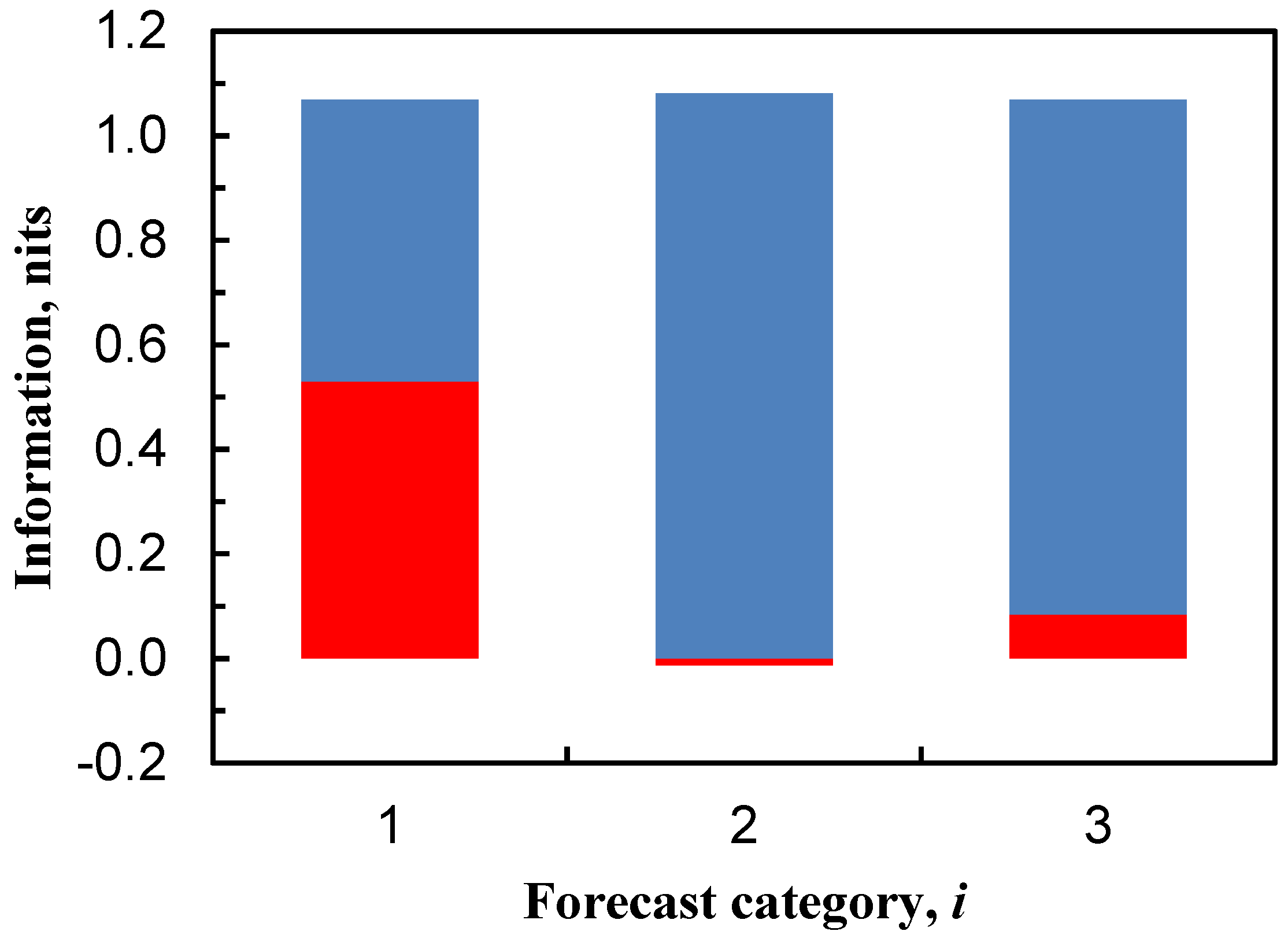
and from Table 1 [using Equation (9)], working in natural logarithms, we calculate H(O|f1) = 0.5382, H(O|f2) = 1.0813, and H(O|f3) = 0.9839 nits. Specific information, denoted IS(fi), is then:
I S ( f i ) = H ( O ) H ( O | f i )
(DelSole [26] refers to this quantity as ‘predictive information’). This quantity may be positive (when H(O) > H(O|fi), in which case uncertainty has decreased), or negative (when H(O) < H(O|fi), in which case uncertainty has increased). For the present example, based on Table 1, the results are illustrated in Figure 2.
Figure 2. For each forecast category i, the bar comprises a red component IS(fi), and a blue component H(O|fi) which together sum to H(O) in each case. The weighted average of red components is equal to IM(O,F) (the Pr(fi) provide the appropriate weights).
Entropy 15 00972 g002
Expanding Equation (10), we have:
I S ( f i ) = j Pr ( o j ) log [ 1 Pr ( o j ) ] j Pr ( o j | f i ) log [ 1 Pr ( o j | f i ) ]
and thus we can see that Equation (6) calculates the expected value of IS(fi); that is to say, expected mutual information is expected specific information over all forecast categories:
I M ( O , F ) = i Pr ( f i ) I S ( f i )

3.4. Relative Entropy

Recall Section 3.1, where we defined the information content of a message that tells us, without error, that an event has occurred. In practice, not all the messages we receive will tell us without error that the event in question has occurred (see, e.g., Figure 1 above). So now we can think of a message as serving to transform a set of prior probabilities into a corresponding set of posterior probabilities. In this case, we can generalize as follows:
i n f o r m a t i o n c o n t e n t o f m e s s a g e = log [ p r o b a b i l i t y o f e v e n t a f t e r m e s s a g e r e c e i v e d p r o b a b i l i t y o f e v e n t b e f o r e m e s s a g e r e c e i v e d ] = log [ Pr ( E | m e s s a g e ) ] log [ Pr ( E ) ] = h [ Pr ( E ) ] h [ Pr ( E | m e s s a g e ) ]
which includes the previous example of the message that tells us without error what has occurred (i.e., Pr(E|message)=1) as a special case. We now generalize Equation (1) in order to calculate expected information content for such a message.
Recall the observed N2O flux categories o1 (‘low’), o2 (‘medium’) and o3 (‘high’), with corresponding probabilities Pr(o1), Pr(o2) and Pr(o3), which we will call the prior (i.e., pre-forecast) probabilities. A message fi is received which serves to transform these prior probabilities into the posterior probabilities Pr(oj|fi), with j Pr ( o j | f i ) = 1 , Pr ( o j | f i ) 0 , j = 1 , 2 , 3. The information content of this message as viewed from the perspective of a particular oj is [from Equation (13)]:
i n f o r m a t i o n c o n t e n t o f m e s s a g e f i = log [ Pr ( o j | f i ) Pr ( o j ) ]
The expected information content of the message fi is I(fi), is the weighted average of the information contents, the weights being the posterior probabilities Pr(oj|fi):
I ( f i ) = j Pr ( o j | f i ) log [ Pr ( o j | f i ) Pr ( o j ) ]
referred to here as the relative entropy (also widely known as the Kullback-Leibler divergence). The quantity I(fi) ≥ 0, and is equal to zero if and only if Pr(oj|fi) = Pr(oj) for all j; thus the expected information content of a message which leaves the prior probabilities unchanged is zero, which is reasonable. For the present example, based on Table 1, the results are illustrated in Figure 3.
Note now that we can re-write Equation (5) as:
I M ( O , F ) = i Pr ( f i ) j Pr ( o j | f i ) log [ Pr ( o j | f i ) Pr ( o j ) ]
so now, recalling Equation (15), we can write:
I M ( O , F ) = i Pr ( f i ) I ( f i )
and thus we can see that Equation (16) calculates the expected value of I(fi); that is to say, expected mutual information is expected relative entropy over all forecast categories.
Thus we have two information quantities that characterize a specific forecast fi, for both of which the expected value is the expected mutual information IM(O,F). Specific information, IS(fi), is based on the difference between two entropies [Equation (10)]. Relative entropy, I(fi), is based on the difference between two information contents [Equations (13) and (14)].
Figure 3. For each forecast category i, the bar comprises a red component I(fi), and a blue component H(O|fi). The weighted average of the sums of the two components is equal to H(O). The weighted average of red components is equal to IM(O,F). In each case the Pr(fi) provide the appropriate weights.
Entropy 15 00972 g003

3.5. A Second Data Set

Here we present a second prediction-realization table based on a boundary line plot for cereal cropping soils from Figure 2 of [16] (Table 2) and then summarize the calculations based on both Table 1 and Table 2 (Table 3).
Table 2. Prediction-realization table based on N=247 observations of N2O flux for cereal cropping soils from Figure 2 of [16]. The boundary lines between forecast emission categories were WFPS(%)+0.76∙T(°C) = 78 (low-medium) and WFPS(%)+0.76∙T(°C) = 90 (medium-high).
Forecast category, fiObserved category, ojRow sums
1. Low2. Medium3. High
1. Low0.78540.03240.00000.8178
2. Medium0.09720.04450.00400.1457
3. High0.01210.02020.00400.0364
Column sums0.89470.09720.00811.0000
Table 3. Summary of information quantities and calculations (working in natural logarithms).
Information quantityEquation (boldface indicates equation used for calculation)Value (nits) for pasture and sugarcane soils data (Table 1)Value (nits) for cereal cropping soils data (Table 2)
H(O)11.06870.3650
H(F)21.09360.5659
H(O,F)31.95850.8430
IM(O,F)4, 5, 6, 7, 12, 16, 170.20380.0879
H(O|F)Component of 60.86490.2772
H(F|O)Component of 70.88980.4780
normalized IM(O,F)80.19070.2407
H(O|f1)90.5382 a,b0.1667
H(O|f2)91.0813 a,b0.7321
H(O|f3)90.9839 a,b0.9369
IS(f1)10, 11 0.5305 a0.1984
IS(f2)10, 11 −0.0126 a−0.3671
IS(f3)10, 11 0.0848 a−0.5718
I(f1)15 0.3428 b0.0325
I(f2)15 0.0442 b0.1882
I(f3)15 0.2388 b0.9305
a see Figure 2; b see Figure 3

4. Results and Discussion

From Table 3, we see that the entropy H(O) for pasture and sugarcane soils is larger than for cereal cropping soils, indicating greater dispersion in the distribution Pr(O) for pasture and sugarcane soils. The expected mutual information IM(O,F) is a measure of association between forecasts and observations. This is larger for pasture and sugarcane soils than for cereal cropping soils, but is difficult to interpret because its maximum value is the entropy H(O). If, instead, we look at the normalized version of IM(O,F), which lies between 0 and 1, we see that the proportion of entropy in O that is explained by the forecaster F is similar for both data sets (see Table 3).
If we look at the relative entropies I(fi) for cereal cropping soils (Table 3), the small value for I(f1) and the large value for I(f3) are notable. In each case, the largest component of I(fi) will arise from the information content of a correct forecast, ln[Pr(oj|fi)/Pr(oj)] (i=j) [from Equation (14)]. From Table 2, for a correct f1 (‘low’) forecast, information content = ln[0.7854/(0.8178∙0.8947)] = 0.0708 nits. From Table 2, we calculate that an f1 forecast provides about 96% correct forecasts, but this is set against the fact that almost 90% correct categorizations could be made just on the basis of o1 without recourse to a forecast. Information content is a measure of the value of a forecast given what we already know. For a correct f3 (‘high’) forecast, information content = ln[0.0040/(0.0364∙0.0081)] = 2.6190 nits. While this is impressively large, it is based on only two o3 observations, of which one was correctly forecast, so should be regarded with caution. For cereal cropping soils, we note also that the specific information values IS(f2) and IS(f3) are negative (Table 3). As almost 90% of the observations were in the o1 category, an f2 forecast results in H(O|f2)>H(O) and an f3 forecast results in H(O|f3)>H(O) (Table 3); in both cases uncertainty is increased.
For pasture and sugarcane soils, the small value for the relative entropy I(f2) is notable (Table 3). From Table 1, for a correct f2 (‘medium’) forecast, information content = ln[0.1513/(0.3653∙0.2878)] = 0.3639 nits, not small enough to provide an explanation for the small value of I(f2) without further investigation. From Table 1, we calculate that an f2 forecast provides about 41% correct forecasts, smaller than for both an f1 forecast (about 82%) and an f3 forecast (about 55%). At the same time, f2 forecasts make up a larger percentage of the total forecasts (about 36%) than f1 (about 35%) or f3 (about 29%). Further, the conditional entropy H(O|f2) is larger than H(O|f1) and H(O|f3); so large, in fact, that an f2 forecast results in H(O|f2)>H(O) and IS(f2) is negative, indicating increased uncertainty (Table 3). Taken together, these results indicate that the small value for the relative entropy I(f2) arises because the f2 forecast category contains relatively large proportions of incorrectly-forecast o1 and o3 observations in addition to the correctly-forecast o2 observations.
On the basis of our analysis, we note that there is a prima facie case for considering boundary line models for N2O flux in which the parameter space is partitioned by a single threshold into two sub-regions. In particular, the advantage of retaining separate medium and high emission categories deserves critical examination. As discussed above:
  • for cereal cropping soils, information properties of the three sub-region model largely depend on the prior (i.e., pre-forecast) probabilities Pr(o1) (≈0.9), Pr(o2) (≈0.1) and Pr(o3) (<0.01) of the observed N2O flux categories o1 (‘low’), o2 (‘medium’) and o3 (‘high’) respectively;
  • for pasture and sugarcane soils, information properties of the three sub-region model indicate that observed N2O flux categories o1 (‘low’), o2 (‘medium’) and o3 (‘high’) are poorly distinguished in the f2 forecast category.
Further:
  • Conen et al. [15] observed that “During most days of the year, emissions tend to be within the ‘low’ range, increasing to ‘medium’ or ‘high’ only after fertilizer applications, depending on soil temperature or WFPS limitations.”
  • Recalling the data set from Figure 1, we note that as in [15], most emissions were in the ‘low’ observed range. The proportions of emissions in the ‘low’ (<10 g N2O-N ha−1 day−1), ‘medium’ (10-100 g N2O-N ha−1 day−1) and ‘high’ (>100 g N2O-N ha−1 day−1) observed ranges were ≈0.68, ≈0.30 and ≈0.02, respectively.
Characterizing the extent to which observed levels of a response variable of interest are correctly or incorrectly forecast is greatly simplified if the parameter space is partitioned by a single threshold. For an example of a boundary line model in which the parameter space is partitioned into two sub-regions, an epidemiological study by De Wolf et al. (Figure 2 in [27]) calculates a model with a single threshold, used in forecasting wheat Fusarium head blight epidemics based on within-season weather data. The decision-theoretic and information-theoretic properties of such binary prediction models in epidemiology have been discussed by Madden [28] and Hughes [22] respectively.

5. Conclusions

The boundary line approach provides a simple and practical alternative to more complex process-based models for the estimation of N2O emissions from soils [15,16]. The boundary line approach categorizes data for observed and forecast emissions; a graphical two-threshold boundary line model can be written as a 3×3 prediction-realization table. Boundary line model data in such a tabular format may be analyzed by information theoretic methods as also applied in, for example, psychology [21], economics [18] and epidemiology [22].
Expected mutual information is a measure of the amount of information about the observations contained in the forecasts, characterizing forecaster performance averaged over all forecast categories. Expected mutual information characterizes the component of entropy H(O) that is associated with forecaster F. A normalized version of expected mutual information, with a range from zero (forecasts are independent of observations) to one (forecasts are perfect), is useful if we want to compare model performance over different data sets. Here, we found that a boundary line approach to forecasting N2O emission ranges from Australian agricultural soils [16] provided a similar level of performance averaged over low, medium and high forecast categories for cereal cropping soils and for pasture and sugarcane soils.
Whereas mutual information characterizes the average performance of a forecaster, specific information IS(fi) and relative entropy I(fi) both characterize aspects of the amount information contained in particular forecasts. Here is an heuristic interpretation in relation to our analysis of boundary line models. After receiving forecast fi, we know more than we did before (assuming forecasts are not independent of observations). For N2O flux categories o1 (‘low’), o2 (‘medium’) and o3 (‘high’), we knew the prior probabilities Pr(o1), Pr(o2) and Pr(o3), and now we know the posterior probabilities Pr(o1|fi), Pr(o2|fi) and Pr(o3|fi). Relative entropy is the expected value of the information content of fi; I(fi) cannot be negative. Now, recall that if all the Pr(oj) had the same value, this would represent maximum uncertainty about N2O flux categories O. Generally, larger H(O) represents more uncertainty. So, if after receiving forecast fi the Pr(oj|fi) are more similar than were the Pr(oj), H(O|fi) will be larger than H(O) and IS(fi) will be negative. This represents an increase in uncertainty having received the forecast fi. When H(O|fi) is smaller than H(O), IS(fi) will be positive; this represents a decrease in uncertainty having received the forecast fi.
Finally, for completeness, we note two related areas of study not discussed in the present article, but of potential future interest in the context of applications of information theory to the analysis and modeling of N2O emissions from soils. First, there is another application of boundary line models, not considered here, where a boundary represents the upper or lower limit of a response variable with variation in the value of an explanatory variable (see, e.g., [29,30]). Second, there is a burgeoning interest in information theory as a basis for weather forecast evaluation (e.g., DelSole [26,31]; Weijs et al. [32] and Tödter and Ahrens [33] are recent contributions). In future, such work may also contribute to the analysis of models of N2O emissions from agricultural soils.

Acknowledgments

The research on prediction of N2O emissions with the boundary line model was funded by the Department of Climate Change and Energy Efficiency (via ex-AGO), Australia. The grassland experimental work was funded by the UK Department for Environment, Food and Rural Affairs (Defra), the Scottish Government, the Department of Agriculture and Rural Development in Northern Ireland and the Welsh Government. SRUC receives grant-in-aid from the Scottish Government.

References

  1. Mosier, A.R.; Duxbury, J.M.; Freney, J.R.; Heinemeyer, O.; Minami, K. Assessing and mitigating N2O emissions from agricultural soils. Climatic Change 1998, 40, 7–38. [Google Scholar] [CrossRef]
  2. IPCC (Intergovernmental Panel on Climate Change). Greenhouse gas emissions from agricultural soils. In Revised 1996 IPCC Guidelines for National Greenhouse Gas Inventories, Volume 3, Greenhouse Gas Inventory Reference Manual; Houghton, J.T., Meira Filho, L.G., Lim, B., Treanton, K., Mamaty, I., Bonduki, Y., Griggs, D.J., Callender, B.A., Eds.; IPCC/OECD/IEA: UK Meteorological Office, Bracknell, UK, 1997. [Google Scholar]
  3. Bouwman, A.F. Direct emissions of nitrous oxide from agricultural soils. Nutr. Cycl. Agroecosys. 1996, 46, 53–70. [Google Scholar] [CrossRef]
  4. Bouwman, A.F.; Boumans, L.J.M.; Batjes, N.H. Emissions of N2O and NO from fertilized fields: Summary of available measurement data. Global Biogeochem. Cy. 2002, 16, 6.1–6.13. [Google Scholar] [CrossRef]
  5. Skiba, U.; Ball, B. The effect of soil texture and soil drainage on emissions of nitric oxide and nitrous oxide. Soil Use Manage. 2002, 18, 56–60. [Google Scholar] [CrossRef]
  6. Flechard, C.R.; Ambus, P.; Skiba, U.; Rees, R.M.; Hensen, A.; van Amstel, A.; van den Pol-van Dasselaar, A.V.; Soussana, J.-F.; Jones, M.; et al. Effects of climate and management intensity on nitrous oxide emissions in grassland systems across Europe. Agr. Ecosyst. Environ. 2007, 121, 135–152. [Google Scholar] [CrossRef]
  7. Abdalla, M.; Jones, M.; Williams, M. Simulation of N2O fluxes from Irish arable soils: effect of climate change and management. Biol. Fert. Soils 2010, 46, 247–260. [Google Scholar] [CrossRef]
  8. Hartmann, A.A.; Niklaus, P.A. Effects of simulated drought and nitrogen fertilizer on plant productivity and nitrous oxide (N2O) emissions of two pastures. Plant Soil 2012, 361, 411–426. [Google Scholar] [CrossRef]
  9. Rees, R.M. Global nitrous oxide emissions: sources and opportunities for mitigation. In Understanding Greenhouse Gas Emissions from Agricultural Management; Guo, L., Gunasekara, A.S., McConnell, L.L., Eds.; ACS Publications: Washington DC, USA, 2012; pp. 257–273. [Google Scholar]
  10. Lesschen, J.P.; Velthof, G.L.; de Vries, W.; Kros, J. Differentiation of nitrous oxide emission factors for agricultural soils. Environ. Pollut. 2011, 159, 3215–3222. [Google Scholar] [CrossRef] [PubMed]
  11. Pappa, V.A.; Rees, R.M.; Walker, R.L.; Baddeley, J.A.; Watson, C.A. Nitrous oxide emissions and nitrate leaching in an arable rotation resulting from the presence of an intercrop. Agr. Ecosyst. Environ. 2011, 141, 153–161. [Google Scholar] [CrossRef]
  12. Del Grosso, S.J.; Parton, W.J.; Mosier, A.R.; Ojima, D.S.; Kulmala, A.E.; Phongpan, S. General model for N2O and N2 gas emissions from soils due to dentrification. Global Biogeochem. Cy. 2000, 14, 1045–1060. [Google Scholar] [CrossRef]
  13. Li, C.S.; Frolking, S.; Frolking, T.A. A model of nitrous oxide evolution from soil driven by rainfall events: 1. Model structure and sensitivity. J. Geophys. Res. 1992, 97, 9759–9776. [Google Scholar] [CrossRef]
  14. Li, C.S.; Frolking, S.; Frolking, T.A. A model of nitrous oxide evolution from soil driven by rainfall events: 2. Model applications. J. Geophys. Res. 1992, 97, 9777–9783. [Google Scholar] [CrossRef]
  15. Conen, F.; Dobbie, K.E.; Smith, K.A. Predicting N2O emissions from agricultural land through related soil parameters. Global Change Biol. 2000, 6, 417–426. [Google Scholar] [CrossRef]
  16. Wang, W.; Dalal, R. Assessment of the boundary line approach for predicting N2O emission ranges from Australian agricultural soils. In Proceedings of the 19th World Congress of Soil Science: Soil Solutions for a Changing World, Brisbane, Australia, 1–6 August 2010; Gilkes, R.J., Prakongkep, N., Eds.; IUSS. Published on DVD, http://www.iuss.org (accessed on 1 March 2013).
  17. Tribus, M.; McIrvine, E.C. Energy and information. Sci. Am. 1971, 225, 179–188. [Google Scholar] [CrossRef]
  18. Theil, H. Economics and Information Theory; North-Holland: Amsterdam, The Netherlands, 1967. [Google Scholar]
  19. Shannon, C.E.; Weaver, W. The Mathematical Theory of Communication; University of Illinois Press: Urbana, IL, USA, 1949. [Google Scholar]
  20. Cover, T.M.; Thomas, J.A. Elements of Information Theory, 2nd ed.; Wiley-Interscience: Hoboken, NJ, USA, 2006. [Google Scholar]
  21. Attneave, F. Applications of Information Theory to Psychology: A Summary of Basic Concepts, Methods, and Results; Holt, Rinehart and Winston: New York, NY, USA, 1959. [Google Scholar]
  22. Hughes, G. Applications of Information Theory to Epidemiology; APS Press: St Paul, MN, USA, 2012. [Google Scholar]
  23. MacDonald, D.K.C. Information theory and its application to taxonomy. J. Appl. Phys. 1952, 23, 529–531. [Google Scholar] [CrossRef]
  24. Agresti, A. Categorical Data Analysis, 3rd ed.; Wiley: Chichester, UK, 2012. [Google Scholar]
  25. Forbes, A.D. Classification-algorithm evaluation: five performance measures based on confusion matrices. J. Clin. Monitor. 1995, 11, 189–206. [Google Scholar] [CrossRef]
  26. DelSole, T. Predictability and information theory. Part I: Measures of predictability. J. Atmos. Sci. 2004, 61, 2425–2450. [Google Scholar]
  27. De Wolf, E.D.; Madden, L.V.; Lipps, P.E. Risk assessment models for wheat Fusarium head blight epidemics based on within-season weather data. Phytopathology 2003, 93, 428–435. [Google Scholar] [CrossRef] [PubMed]
  28. Madden, L.V. Botanical epidemiology: some key advances and its continuing role in disease management. Eur. J. Plant Pathol. 2006, 115, 3–23. [Google Scholar] [CrossRef]
  29. Schmidt, U.; Thöni, H.; Kaupenjohann, M. Using a boundary line approach to analyze N2O flux data from agricultural soils. Nutr. Cycl. Agroecosys. 2000, 57, 119–129. [Google Scholar] [CrossRef]
  30. Farquharson, R.; Baldock, J. Concepts in modelling N2O emissions from land use. Plant Soil 2008, 309, 147–167. [Google Scholar] [CrossRef]
  31. DelSole, T. Predictability and information theory. Part II: Imperfect forecasts. J. Atmos. Sci. 2005, 62, 3368–3381. [Google Scholar]
  32. Weijs, S.; Van Nooijen, R.; Van de Giesen, N. Kullback-Leibler divergence as a forecast skill score with classic reliability-resolution-uncertainty decomposition. Mon. Weather Rev. 2010, 138, 3387–3399. [Google Scholar] [CrossRef]
  33. Tödter, J.; Ahrens, B. Generalization of the ignorance score: continuous ranked version and its decomposition. Mon. Weather Rev. 2012, 140, 2005–2017. [Google Scholar] [CrossRef]