1. Introduction
Fundamental to hydraulic modeling of natural rivers, including modeling of sediment and contaminant transport, design of channels and river training works, design of hydraulic structures, development of a rating curve, and so on, is the velocity distribution. In general, velocity in open channels varies in three dimensions: along flow depth, width, and length. In a given cross-section, the velocity varies along the flow depth and along the transverse direction or width. Along the flow depth it varies from zero at the channel bed to a maximum value which, depending on channel geometric characteristics, exists either at the water surface or some distance below it. Along the transverse direction, it varies from zero at one boundary to a maximum value at some point in the flow domain and then declines to zero at the other boundary. The non-uniformity in the distribution of velocity from the bed to the open water surface and from one boundary to the other is caused by shear stresses.
It is known that velocity is subject to the uncertainties due to both the intrinsic randomness and our inability to interpret the complex interactions. The empirical 1D power law velocity distribution is not capable of incorporating these uncertainties. More modern approaches, mainly based on the concept of entropy, as in the fields of hydraulics and hydrology [
1,
2], consider velocity as a probabilistic variable, taking into account this uncertainty. Following Chiu [
3], it is plausible to consider time-averaged velocity as a probabilistic variable, derive the probability distribution of velocity and then derive the velocity distribution. Chiu [
3] proposed the entropy theory for deriving the velocity distribution which has since been employed by Chiu and his associates [
3,
4,
5,
6,
7,
8,
9,
10], as well others [
11,
12,
13,
14,
15,
16,
17]. Some of these investigations dealt with 1D and some with 2D velocity distributions. Although the 2D velocity distribution proposed by Chiu [
4] has been used in a number of theoretical investigations, its practical usefulness is inhibited by the many parameters it contains. Moramarco
et al. [
18] simplified the 2D model by applying it to several verticals, but still it contains too many parameters. Also employing the entropy theory, Marini
et al. [
19] developed a generic 2D velocity distribution, which involves the geometry of the cross-section, average velocity, and the position and value of maximum velocity. The model does not require calibration and was successfully tested by comparing theoretical values with experimental measurements [
20].
This approach is also employed in the present paper, aiming at deriving the 2D power law velocity distribution using the Shannon entropy and comparing it with the entropy-based logarithmic velocity distribution developed by Marini
et al. [
19].
2. Derivation of 2D Power Law Velocity Distribution
It is assumed that the time-averaged velocity can be considered as a random variable [
21]. The entropy-based approach for deriving the 2D power law velocity distribution entails maximizing the Shannon entropy subject to specified constraints and hypothesizing a relation between the cumulative distribution function (CDF) of
u and flow depth
y. The Shannon entropy [
22] of velocity
u,
S(
u), can be expressed as:
where
f(
u) is the probability density function (PDF) of
u, and
umax is the maximum velocity. Two constraints must been defined to derive the 1D power law velocity distribution:
which defines the PDF of
u [
5], and:
which represents the mean of the logarithmic velocity [
23]. Since the constraints given by Equations (2) and (3) also hold in the 2D domain, a general equation for the velocity PDF was obtained. Following the approach proposed by Singh [
24] for 1D domain, maximizing entropy according to the principle of maximum entropy (POME) [
25,
26,
27] and using the method of Lagrange multipliers, the entropy-based PDF of
u can be written as:
where λ
1 and λ
2 are the Lagrange multipliers, calculated according to Equations (2) and (3).
To derive the 2D velocity distribution, let us consider a 2D domain (
x,
y), with
x denoting the transverse direction and
y the vertical direction measured from the bed, upward positive. Let
u =
u(
x,
y) be the velocity distribution,
f[
u(
x,
y)] the PDF and
F[
u(
x,
y)] the CDF. It is convenient to assume
v = ln(
u) [
i.e.,
u = exp(
v)]. Following the methodology developed by Marini
et al. [
19] and taking the partial derivatives of
F(
u) with respect to
x and
y, we obtain:
Using Equation (4), Equations (5) can be rewritten as:
Denoting λ
2+1 =
n, Equations (6) can be rewritten as:
Setting exp(
nv) =
w, the partial derivatives of
w with respect to
x and
y can be cast as:
Substituting Equations (8) into Equations (7), the following system of equations is obtained:
Equations (9) can be integrated using the Leibnitz rule that states:
Because the point (0, 0) lies on a contour in the solution domain,
u at this point is equal to 0 and
v = ln(
u) = −∞. Consequently, the right hand side of Equation (10) becomes:
The definite integral on the left side of Equation (10) is calculated at a generic point (
) identified by the mean of a polygonal curve that starts from (0, 0), passes across (
) and ends at (
), so that:
in which (
) represents a point of the solution domain. The right hand side of Equation (12) can be equated to the right hand side of Equation (11) to obtain:
Because
w(
x,
y) = exp(
nv), Equation (13) is rewritten as:
and recalling that
v = ln(
u), we obtain the expression of
u(
x,
y):
Equation (15) contains two Lagrange multipliers
λ1 and
λ2, which can be calculated using Equations (2) and (3). Inserting Equation (4) into Equation (2) and integrating, one obtains:
Combining Equations (15) and (16) we obtain the equation representing the 2D velocity distribution:
Equation (17) is the power law 2D velocity distribution, which depends on
umax,
n, and the 2D CDF. The derived equation formally coincides with the equation obtained by Singh [
24] for 1D domain, although in this case
F is a function of
x and
y.
Parameter
n can be calculated using the constraint given by Equation (2), resulting in the following equation [
24]:
where
f is given, for the power law equation, by Equation (4). As an alternative, following the approach proposed by Marini
et al. [
19],
n can be calculated from the definition of average channel velocity
uav:
where
A is the channel cross section. As pointed out in the literature, Equation (18) refers to the mean of the logarithmic velocity distribution, whereas Equation (19) considers the average logarithmic velocity in the channel cross section. Unlike
ū, the average channel velocity has a straightforward physical meaning, and consequently it can be more effective to calculate parameter
n.
3. Comparison with Entropy-Based Logarithmic 2D Velocity Distribution
Equation (17) represents an effective way to estimate velocity distribution in a generic 2D domain if the CDF is properly defined. Starting from the same hypothesis, but using a different constraint equation than Equation (2), Marini
et al. [
19] obtained the following equation (logarithmic model):
Similar to Equation (17), Equation (19) depends only on
umax, an entropic parameter (here called
G), and the 2D CDF. Parameter
G can be calculated using the following equation, depending on the mean of velocity distribution and the maximum velocity [
3]:
or considering again the definition of average channel velocity:
For both Equations (17) and (20), 1D and 2D domains can be considered, depending on the assumed CDF. The velocity distributions inferred from the proposed formulation were analyzed for different configurations and compared with Equation (20) in what follows.
3.1. 1D Velocity Distribution and Maximum Velocity on the Water Level
The case of a wide channel geometry (hence the ratio
H/
B between the water depth
H and the channel width
B tends to zero) is analyzed first. Consequently, only vertical velocity was considered. If the maximum velocity occurs for
y =
H, it is well-known [
3] that
F(
u) =
y/
H. Equation (17) becomes:
and
n can be calculated from the following equation, derived from integration of Equation (19):
If Equation (20) is used with the same
F(
u), one obtains:
in which
G can be calculated by means of Equation (22).
The following data were considered in the example:
H = 1 m;
umax = 1 m/s;
uav =
ū = 0.8 m/s, resulting in
G = 4.8 from Equation (20) and 1/
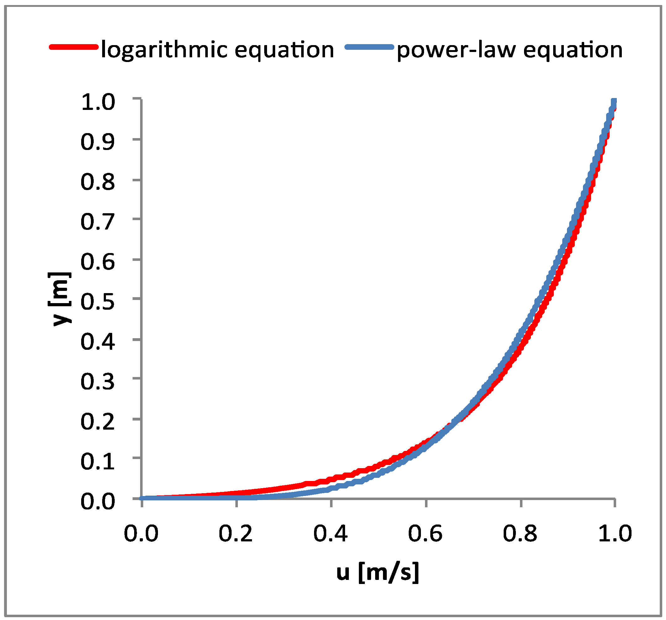
n = 0.25 from Equation (22). The velocity profiles obtained from the power law velocity distribution [Equation (17)] and the logarithmic velocity distribution [Equation (18)] were almost the same (negligible differences), as shown in
Figure 1.
Figure 1.
Velocity profiles calculated using Equations (17) and (20) for 1D domain and y0 = H.
Figure 1.
Velocity profiles calculated using Equations (17) and (20) for 1D domain and y0 = H.
3.2. 1D Velocity Distribution and Maximum Velocity below the Water Level
In this case, the channel geometry of the previous example was used, except for the point where the maximum velocity occurs, which is located at a distance
y0 = 0.8 m from the bed channel. Also in this case, the CDF is well-known [
5]:
and Equation (17) becomes:
and from Equation (19) one obtains 1/
n = 0.81. With the same
F(
u), Equation (20) becomes:
in which
G can be calculated, again, using Equation (22), resulting in
G = 0.55. The velocity profiles inferred from the two distributions were almost identical, as shown in
Figure 2.
Marini
et al. [
19] analyzed the same configuration as a special case of the 2D velocity distribution, thus proposing the following CDF equation:
Figure 2.
Velocity profiles calculated using Equations (17) and (20) for 1D domain,
y0 <
H and
F(
u) proposed by Chiu [
5].
Figure 2.
Velocity profiles calculated using Equations (17) and (20) for 1D domain,
y0 <
H and
F(
u) proposed by Chiu [
5].
Figure 3 shows the velocity profiles obtained using Equation (27) for
F(
u), resulting again in excellent agreement.
Figure 3.
Velocity profiles calculated using Equations (17) and (20) for 1D domain,
y0 <
H and
F(
u) proposed by Marini
et al. [
19].
Figure 3.
Velocity profiles calculated using Equations (17) and (20) for 1D domain,
y0 <
H and
F(
u) proposed by Marini
et al. [
19].
3.3. 2D Velocity Distribution where Maximum Velocity Occurs below Water Level
The 2D domain was analyzed, considering a rectangular channel with symmetrical velocity distribution with respect to the vertical axis. For this configuration Marini
et al. [
19] proposed the following CDF:
Consequently, Equation (17) becomes:
and
n can be calculated using Equation (19). With the same
F(
u), Equation (20) becomes:
and
G can be calculated using Equation (22), in which the average channel velocity can be calculated from the definition of cross-sectional average velocity for the rectangular channel as:
Assuming
H = 1 m;
B = 1 m;
y0 = 0.8 m;
umax = 1 m/s;
uav = 0.8 m/s, we obtain 1/
n = 0.64 from Equation (19) and
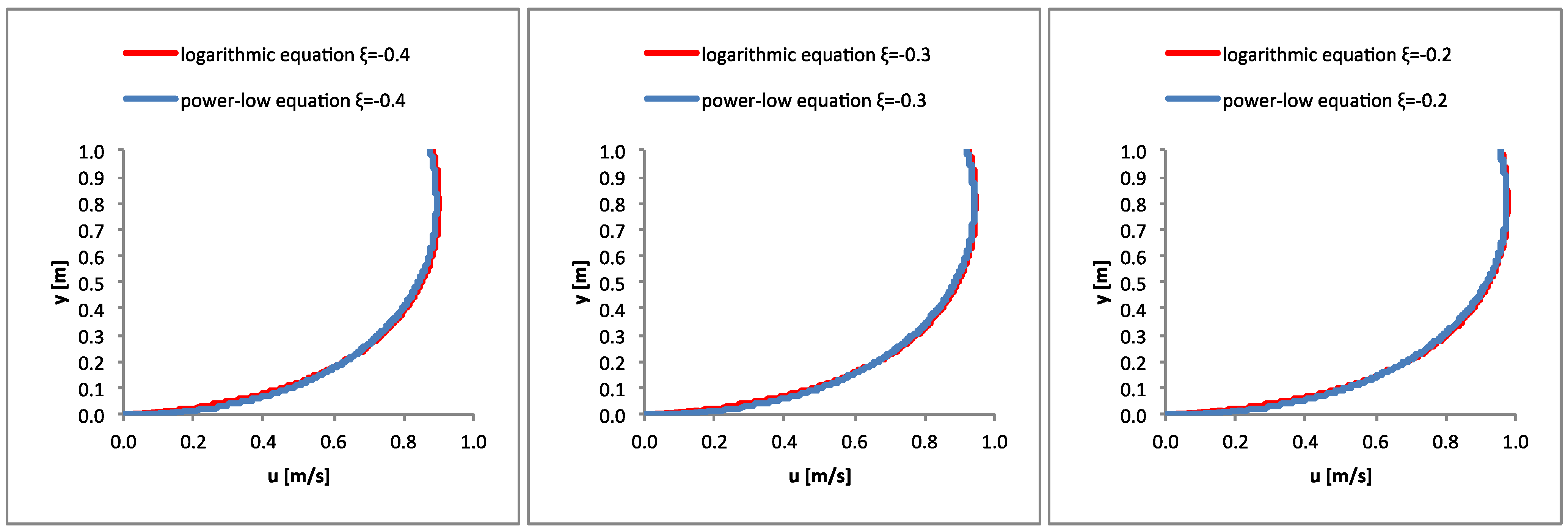
G = 1.22 from Equation (30). The velocity profiles at different abscissas were plotted in
Figure 4, resulting in an excellent agreement.
Figure 4.
Velocity profiles calculated using Equations (17) and (20) for 2D domain (rectangular cross section).
Figure 4.
Velocity profiles calculated using Equations (17) and (20) for 2D domain (rectangular cross section).


