Curvature Entropy for Curved Profile Generation

Abstract
:1. Introduction
2. Definition of Macroscopic Shape Information
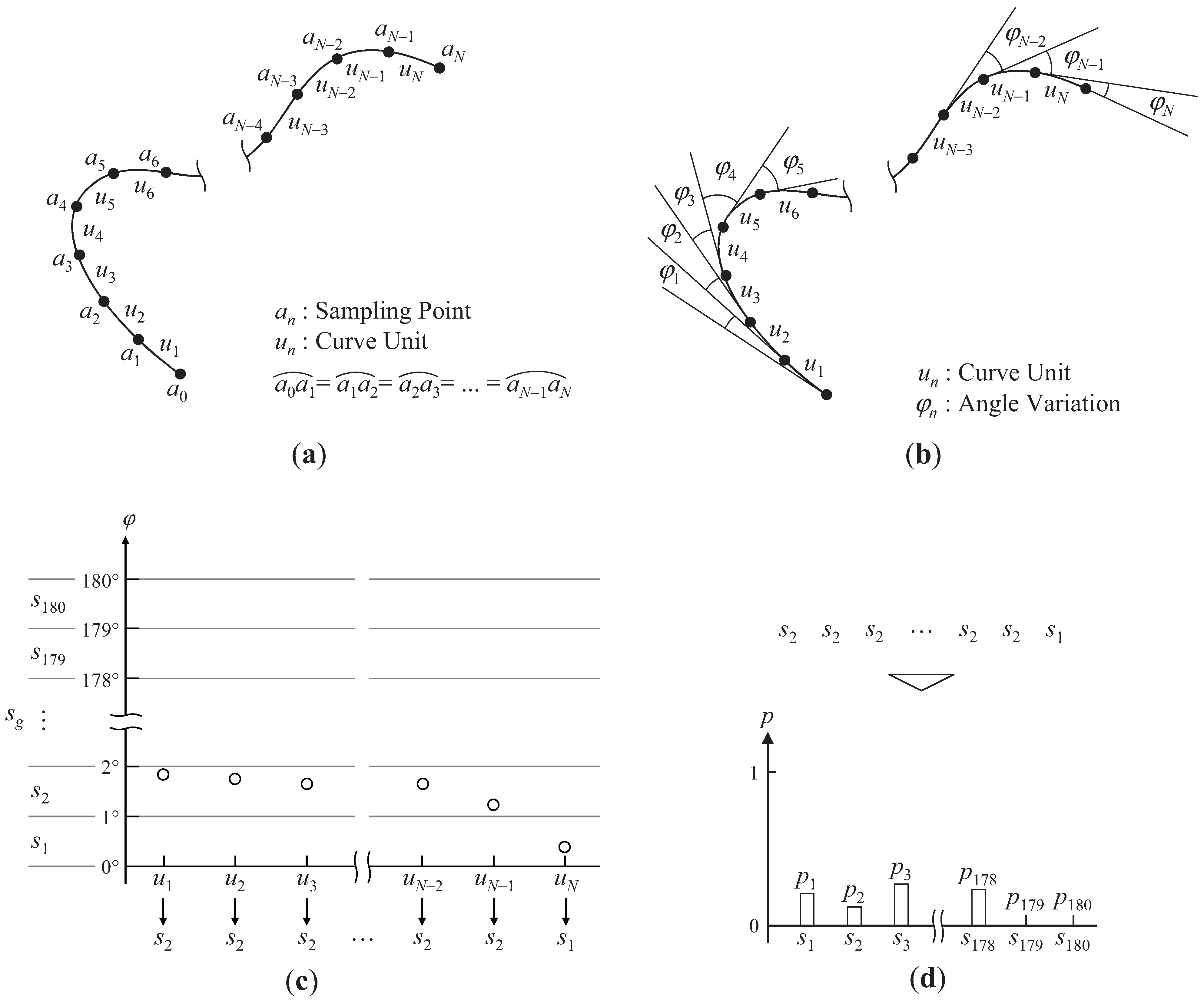
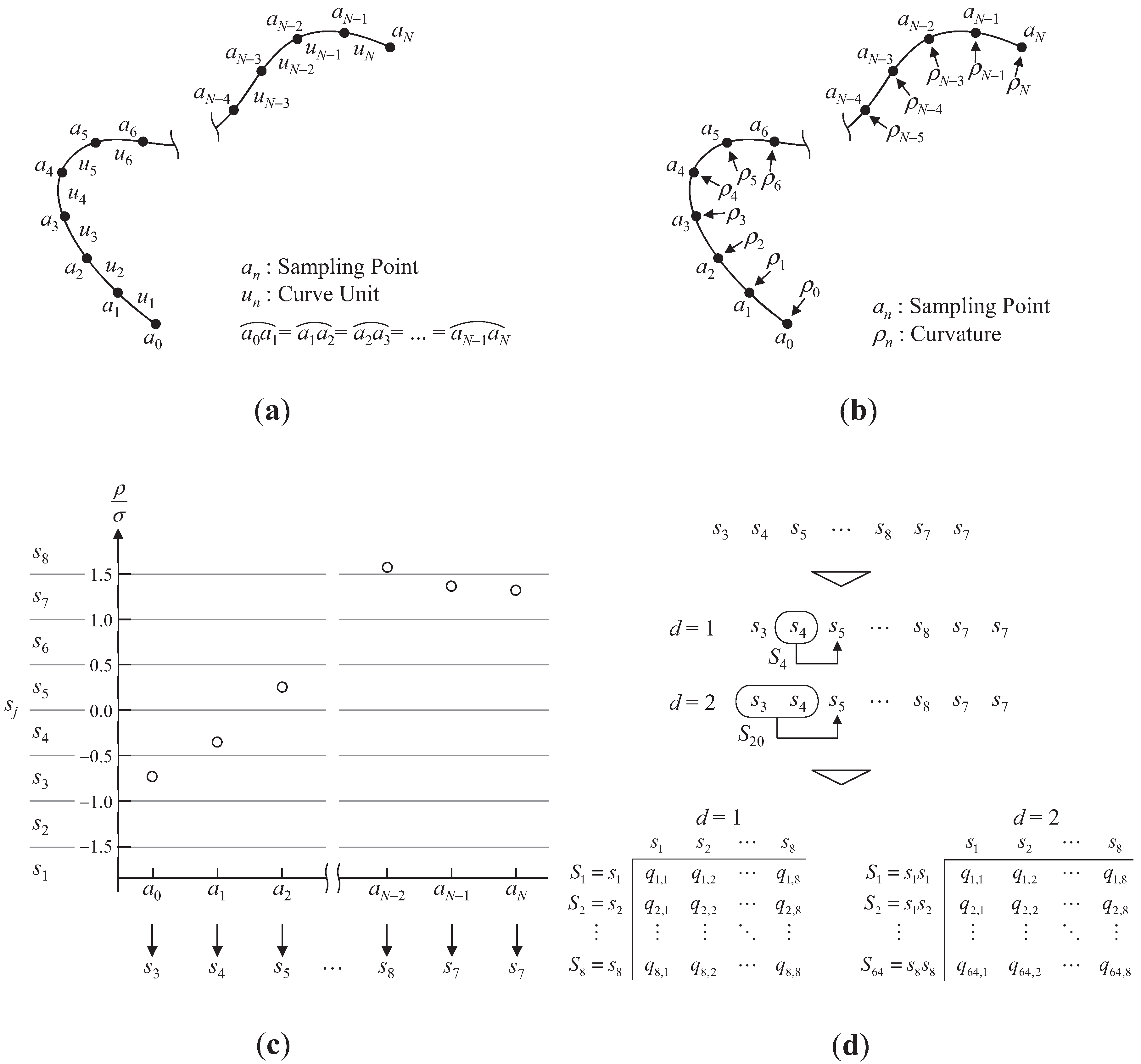
2.1. Angle Variation
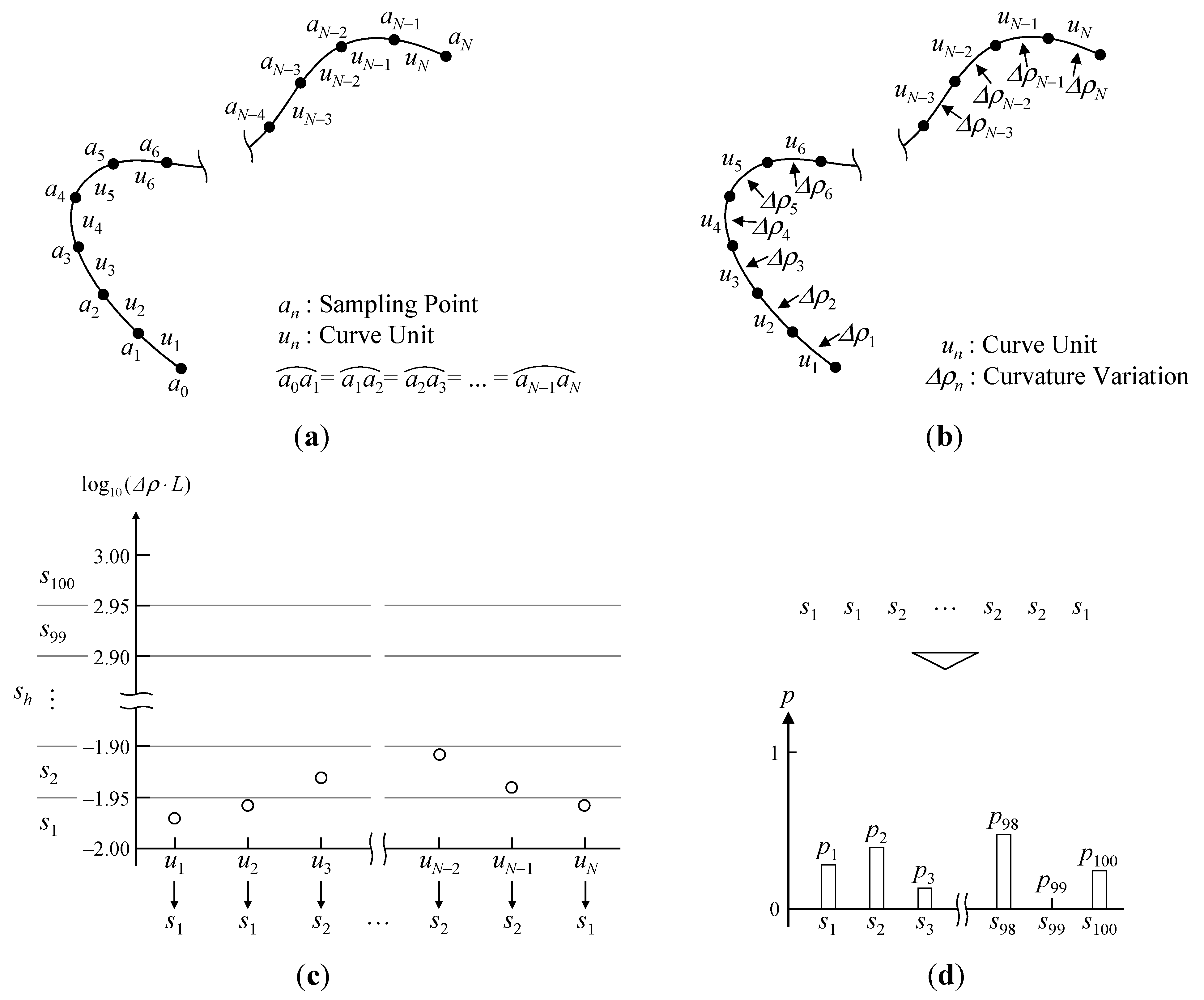
2.2. Curvature Variation


3. Characteristic Analysis of Shape Information in Basic Curved Profiles
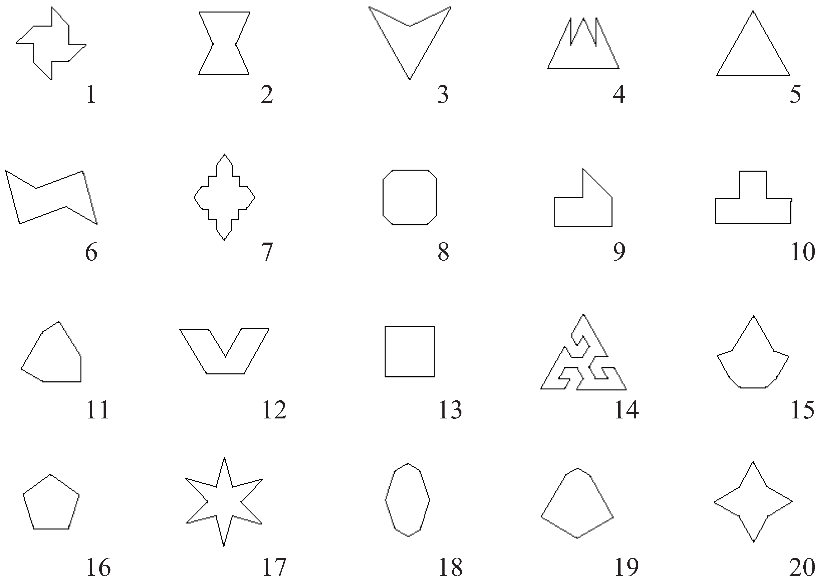
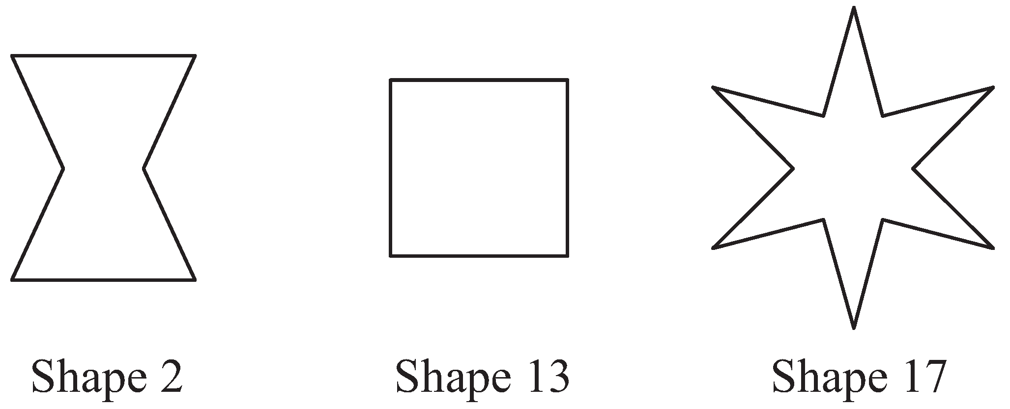
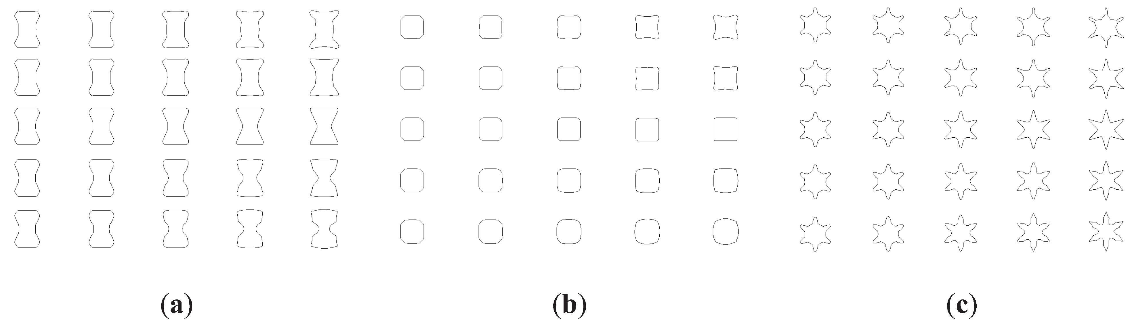
3.1. Description of Basic Curved Profiles

| 1. Circumference | 6. Average width |
| 2. Area | 7. Inclusiveness length |
| 3. X maximum width | 8. Maximum radius vector |
| 4. Y maximum width | 9. Minimum radius vector |
| 5. Roundness | 10. Average radius vector |


3.2. Cognition Experiment of the Curved Profile
- (1)
- Method: semantic differential method (7 stages)
- (2)
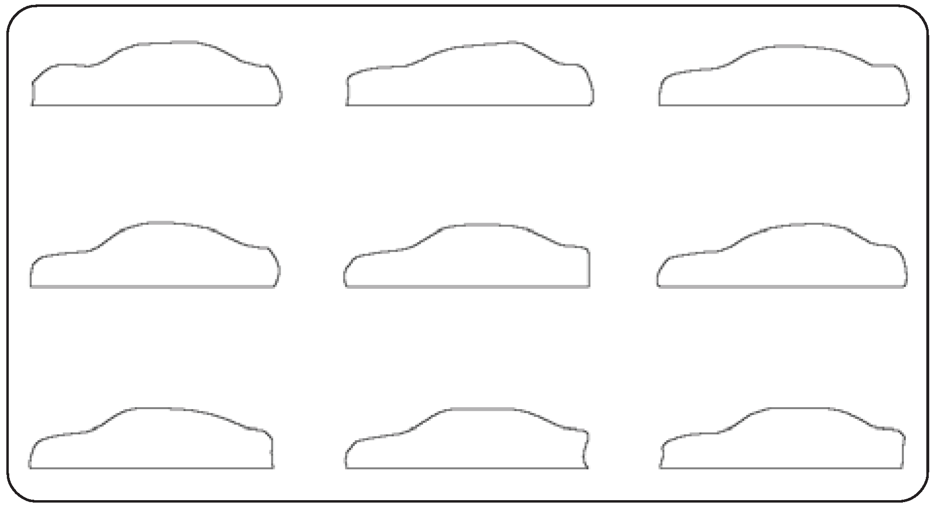
- Samples: 75 samples (basic curved profiles shown in Figure 10)
- (3)
- Evaluation items: 6 items (refer to Table 2)
- (4)
- Examinees: 12 students in their early 20s
| 1. Complex | 4. Light |
| 2. Rectilinear | 5. Fresh |
| 3. Beautiful | 6. Hard |
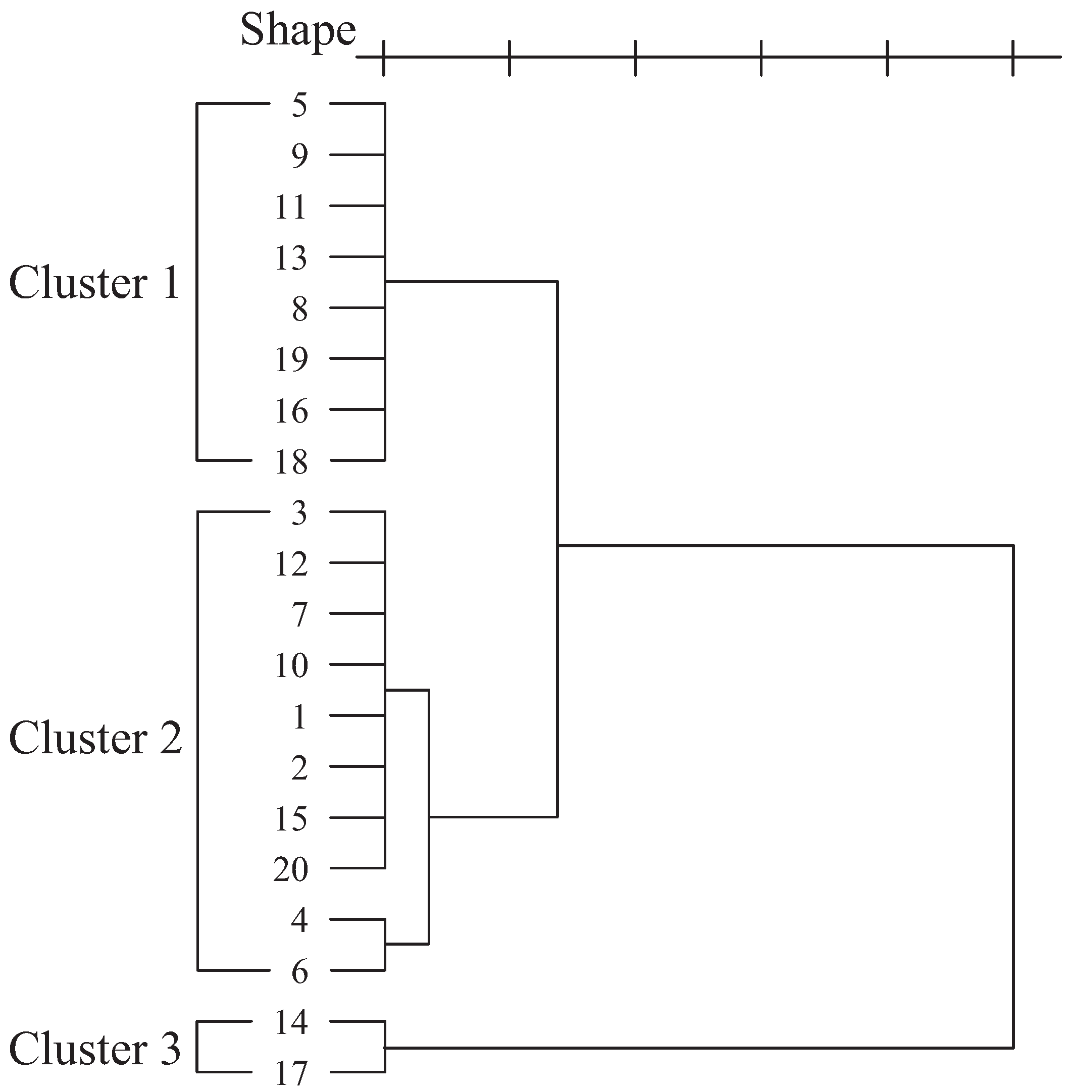
3.3. Analysis
3.3.1. Relationship between Microscopic and Macroscopic Shape Information
| Shape-information | 1st principal component | 2nd principal component | 3rd principal component | 4th principal component | 5th principal component |
|---|---|---|---|---|---|
| Maximum radius vector | 0.981 | 0.065 | −0.028 | −0.065 | −0.106 |
| Inclusiveness length | 0.954 | 0.229 | −0.052 | −0.103 | −0.130 |
| Angle expected value | −0.950 | −0.219 | 0.136 | 0.119 | 0.027 |
| Circumference | −0.947 | −0.181 | 0.060 | −0.108 | 0.021 |
| Average width | 0.846 | 0.502 | −0.081 | −0.090 | 0.006 |
| Roundness | 0.829 | 0.524 | −0.099 | −0.073 | −0.042 |
| Angle entropy | −0.786 | −0.408 | 0.352 | 0.020 | −0.073 |
| X maximum width | 0.265 | 0.913 | −0.099 | 0.208 | 0.185 |
| Minimum radius vector | 0.435 | 0.863 | −0.112 | 0.194 | 0.075 |
| Y maximum width | 0.430 | 0.685 | −0.022 | −0.452 | 0.254 |
| Curvature expected value | 0.058 | −0.074 | −0.963 | −0.127 | −0.066 |
| Curvature entropy | −0.182 | −0.271 | 0.910 | −0.082 | −0.034 |
| Average radius vector | −0.075 | 0.161 | 0.053 | 0.937 | 0.242 |
| Area | −0.165 | 0.223 | 0.036 | 0.223 | 0.928 |
| Contribution ratio (%) | 57.5 | 16.1 | 12.3 | 7.0 | 3.9 |
| Accumulation contribution ratio (%) | 57.5 | 73.6 | 85.9 | 92.9 | 96.8 |
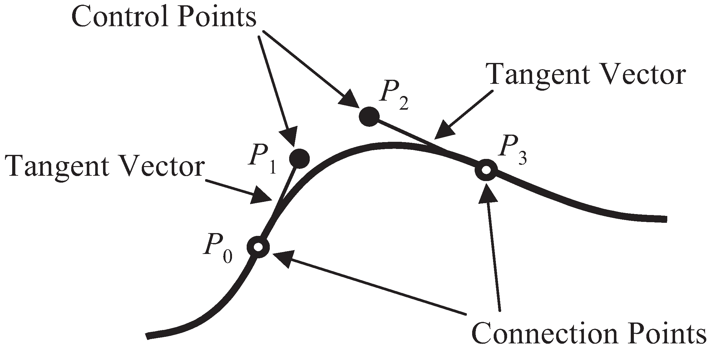
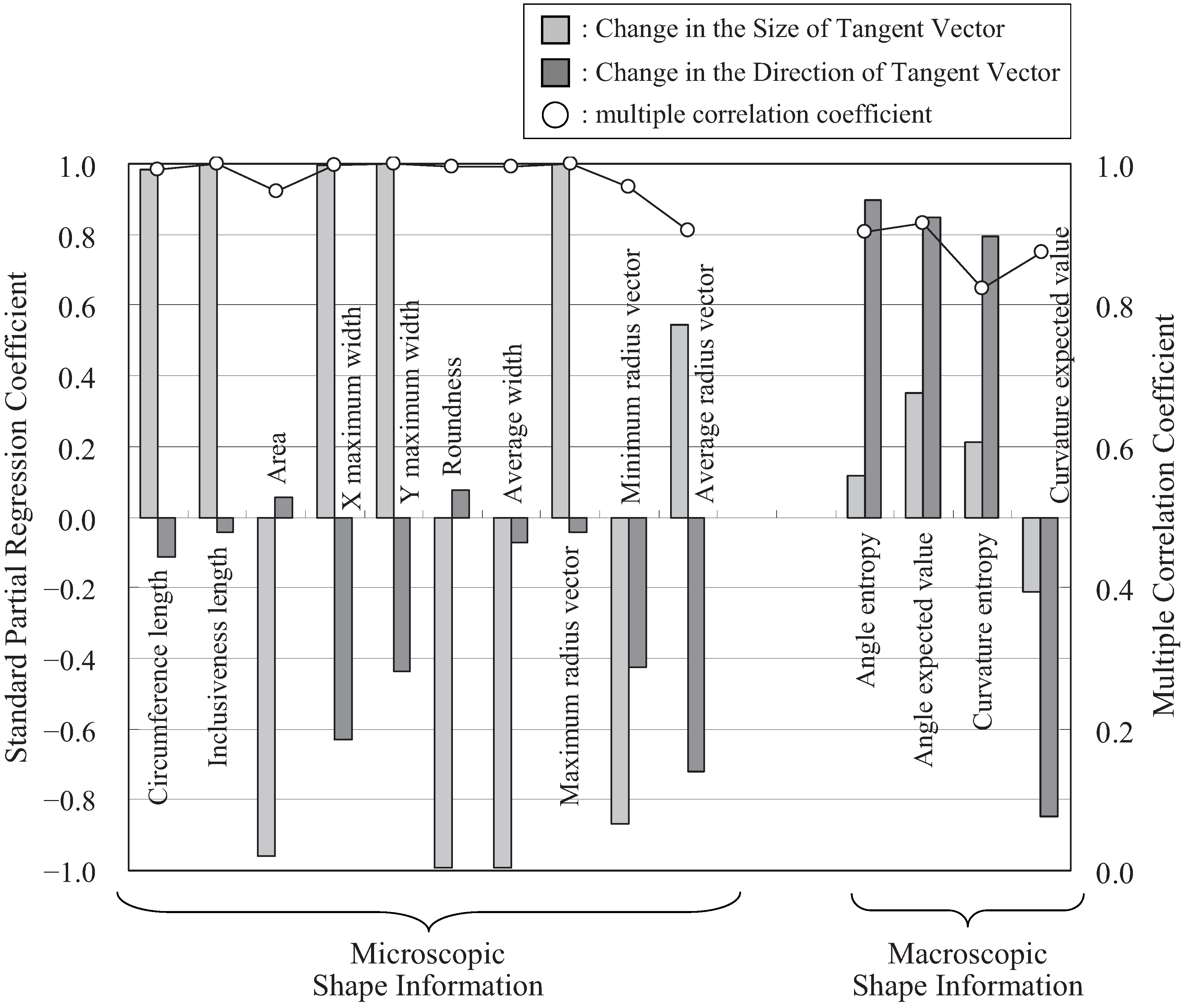
3.3.2. Relationship between the Tangent Vector and Shape Information
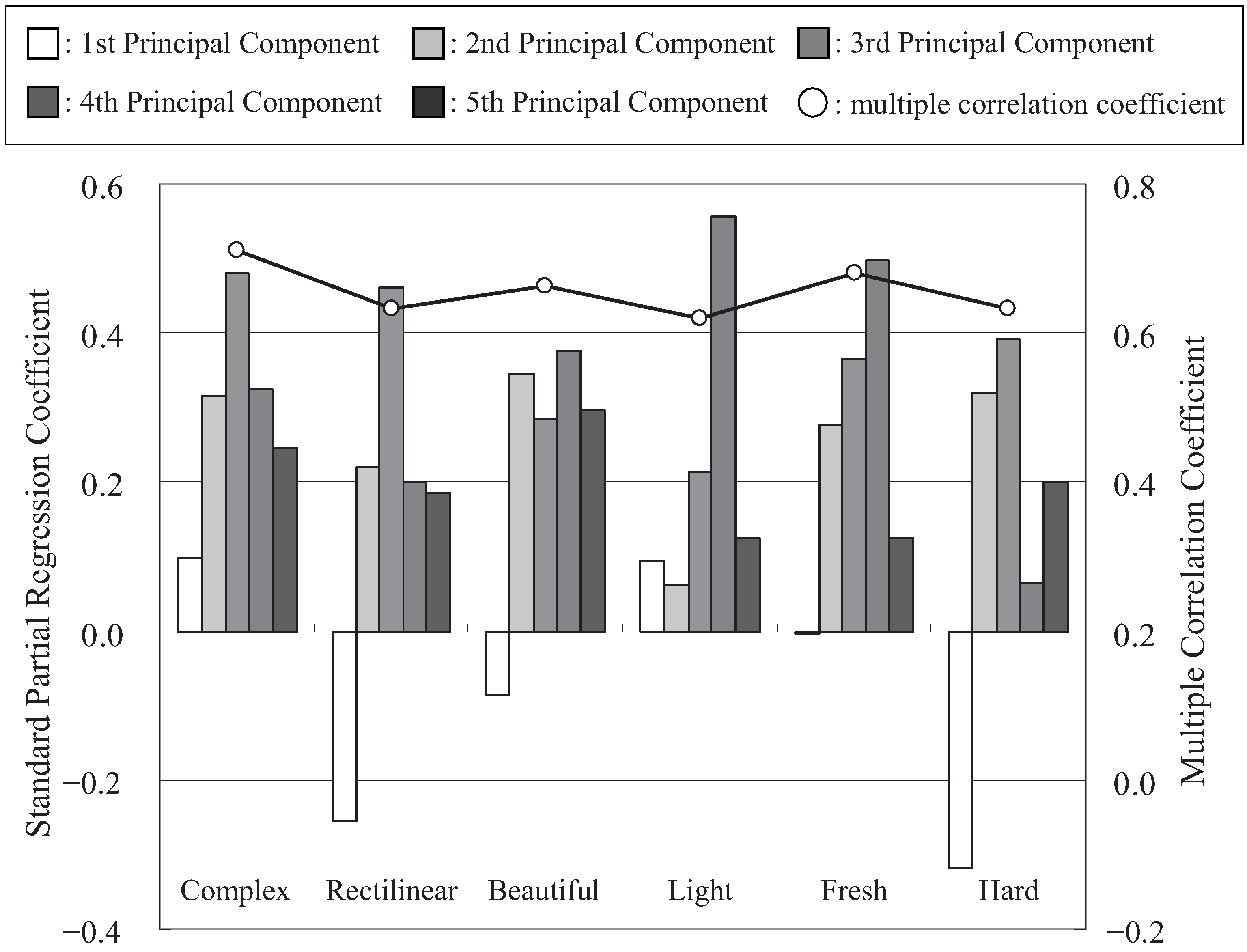
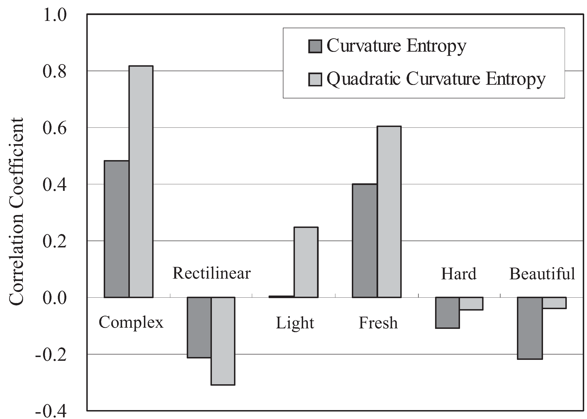
3.3.3. Relationship between Shape Information and Cognition Information

4. Improvement of the Macroscopic Shape Information
4.1. Definition of the Quadratic Curvature Entropy

4.2. Relationship between Microscopic Shape Information and Quadratic Curvature Entropy
| Shape-information | 1st principal component | 2nd principal component | 3rd principal component | 4th principal component | 5th principal component |
|---|---|---|---|---|---|
| Circumference | −0.948 | 0.119 | −0.039 | 0.094 | 0.221 |
| Maximum radius vector | 0.878 | −0.083 | 0.317 | −0.273 | −0.191 |
| Inclusiveness length | 0.866 | 0.003 | 0.341 | −0.296 | −0.203 |
| Average width | 0.788 | 0.118 | 0.517 | −0.243 | −0.179 |
| Roundness | 0.780 | 0.048 | 0.510 | −0.300 | −0.191 |
| Minimum radius vector | −0.041 | 0.973 | −0.080 | −0.113 | −0.034 |
| X maximum width | −0.430 | 0.817 | −0.193 | 0.315 | 0.019 |
| Y maximum width | 0.466 | 0.790 | 0.308 | 0.075 | −0.207 |
| Average radius vector | −0.354 | 0.100 | −0.867 | 0.256 | 0.185 |
| Area | −0.366 | 0.080 | −0.275 | 0.869 | 0.152 |
| Quadratic curvature entropy | −0.488 | −0.179 | −0.254 | 0.190 | 0.793 |
| Contribution ratio (%) | 41.374 | 21.130 | 16.141 | 11.767 | 8.418 |
| Accumulation contribution ratio (%) | 41.374 | 62.504 | 78.645 | 90.412 | 98.830 |
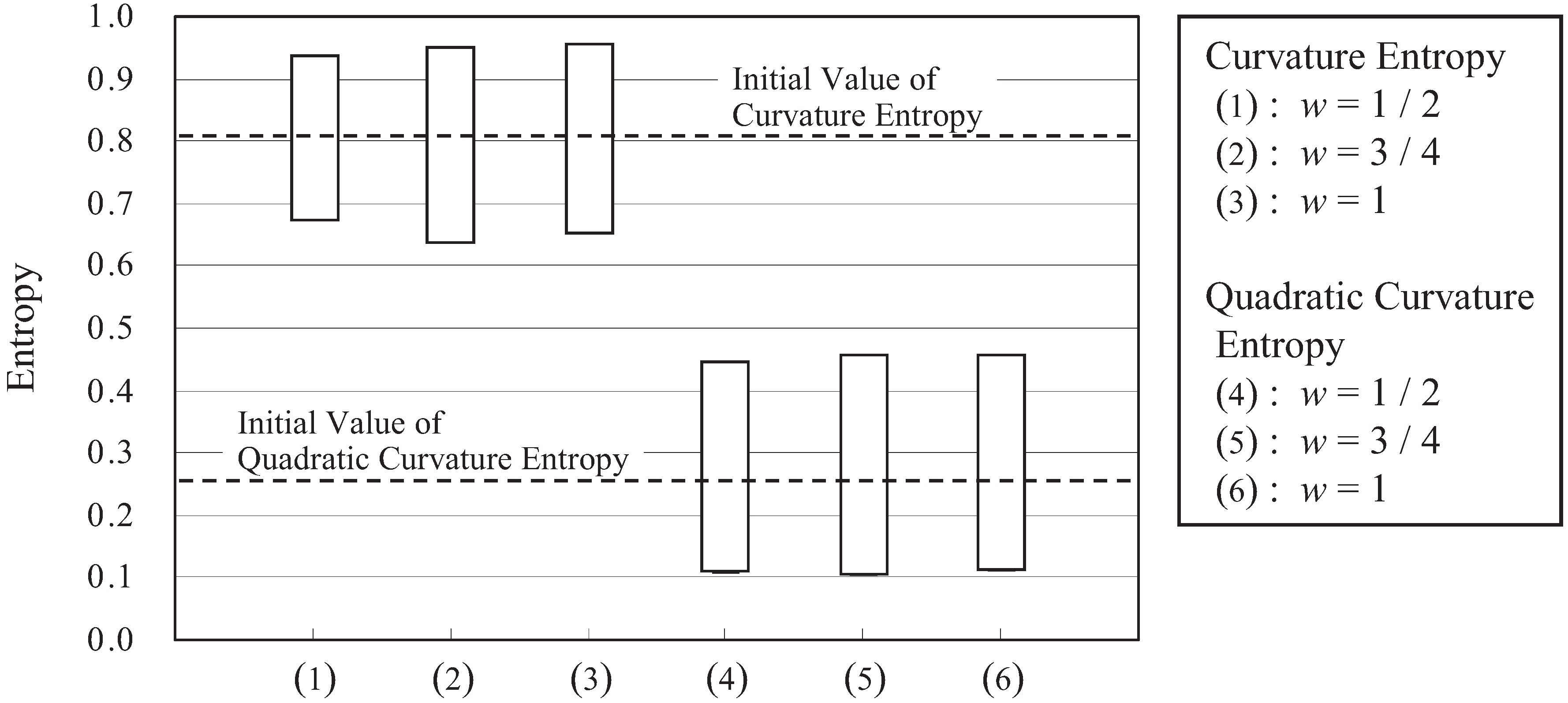
4.3. Relationship between Shape Information, Including Quadratic Curvature Entropy, and Cognition Information

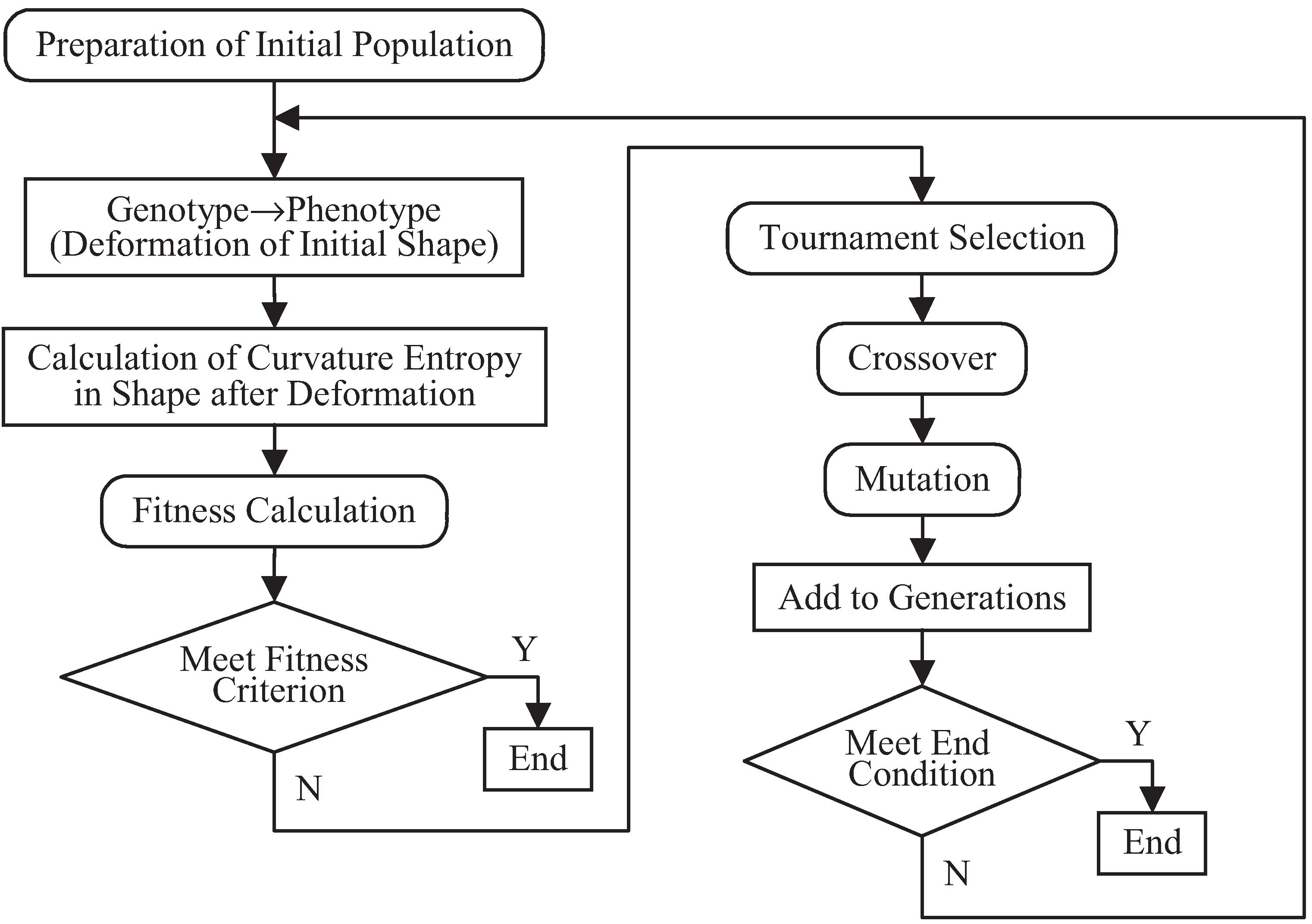
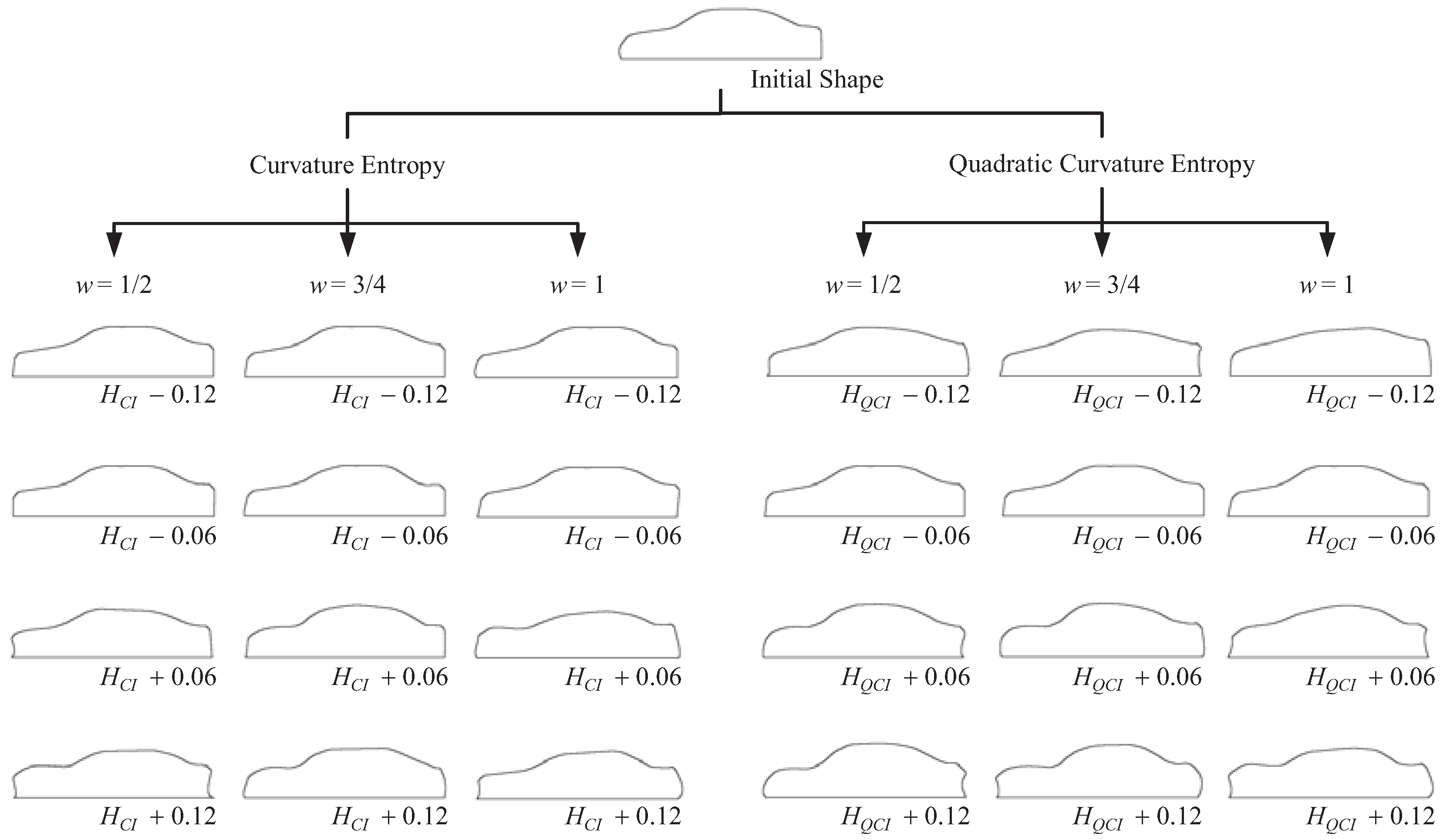
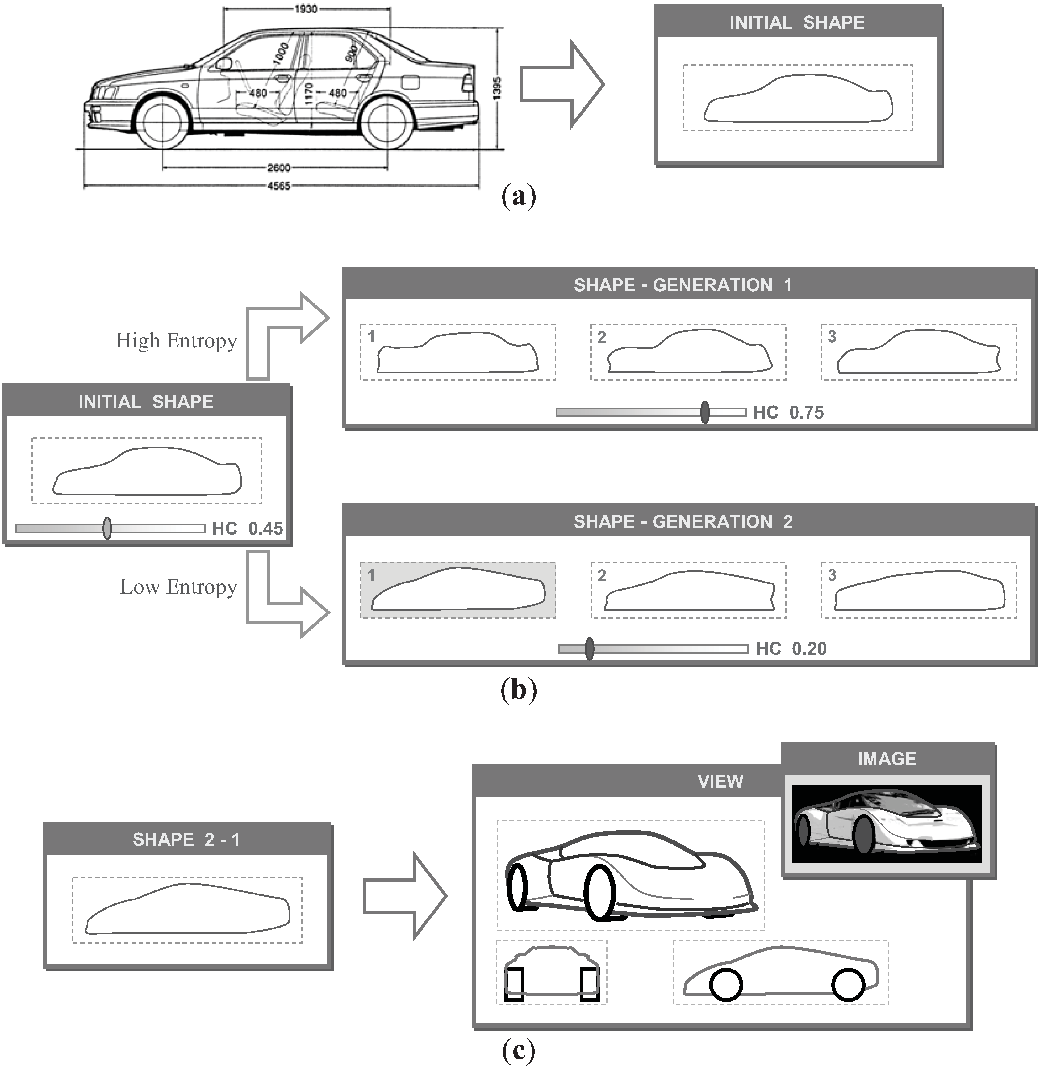
5. Shape Generation Method
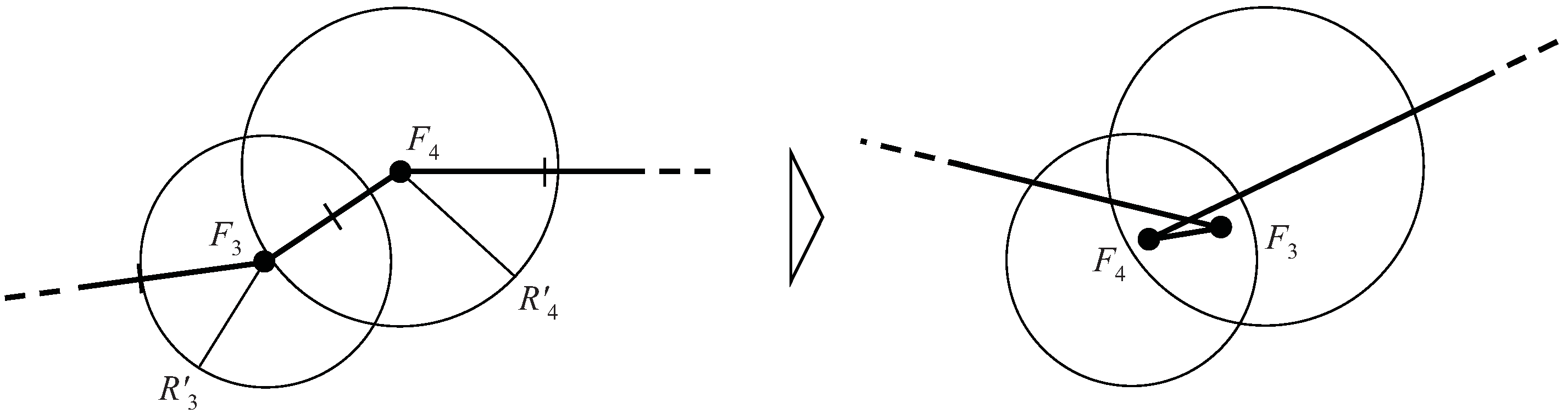
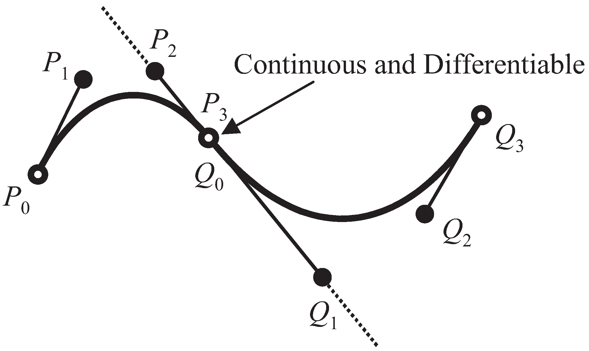
5.1. Description of the Initial Shape
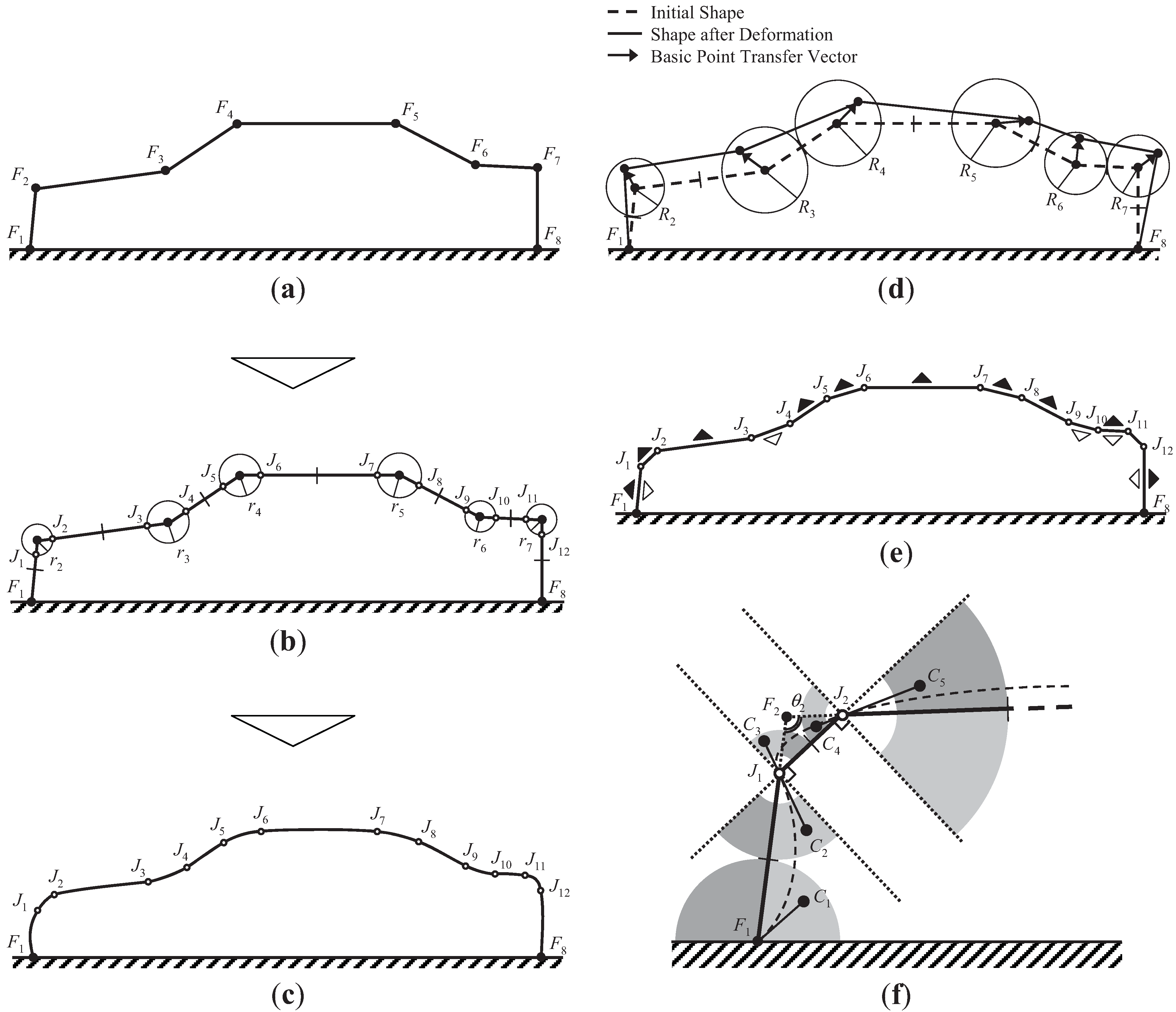

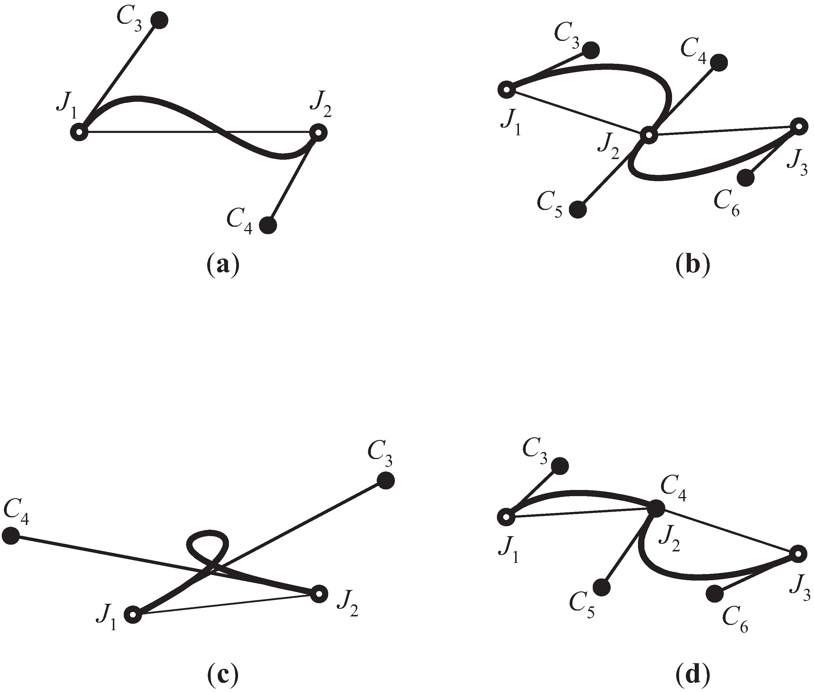
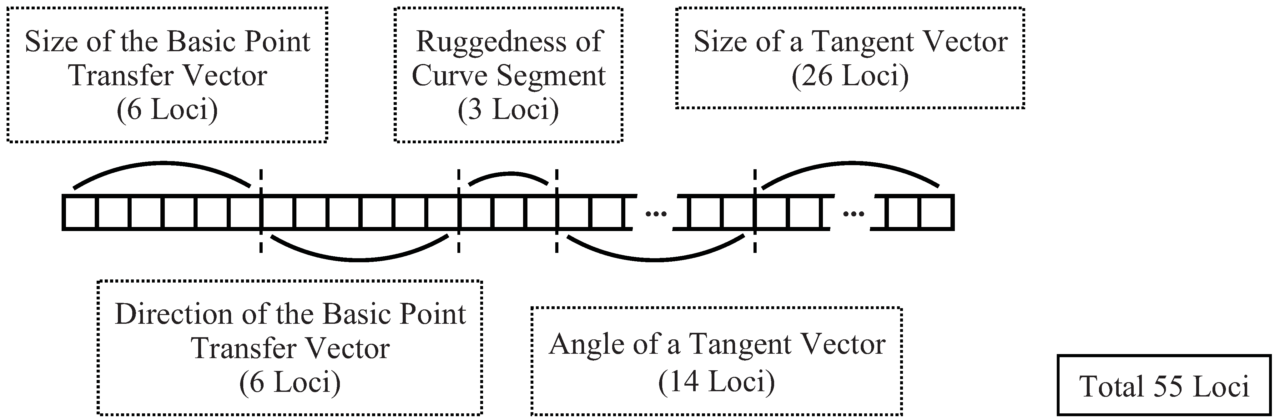
5.2. Coding in a Genetic Algorithm
- (1)
- Position of basic point:where w is a degree of freedom in shape generation. xk and yk are x and y directional components of the basic point transfer vector, respectively, and xIk and yIk are x and y coordinates of the basic point in the initial shape, respectively.
- (2)
- Ruggedness of a curve segment:If 0 ≤ nreal < 0.5, the curve segment is convex. Otherwise (0.5 ≤ nreal ≤ 1:) the curve segment is concave.
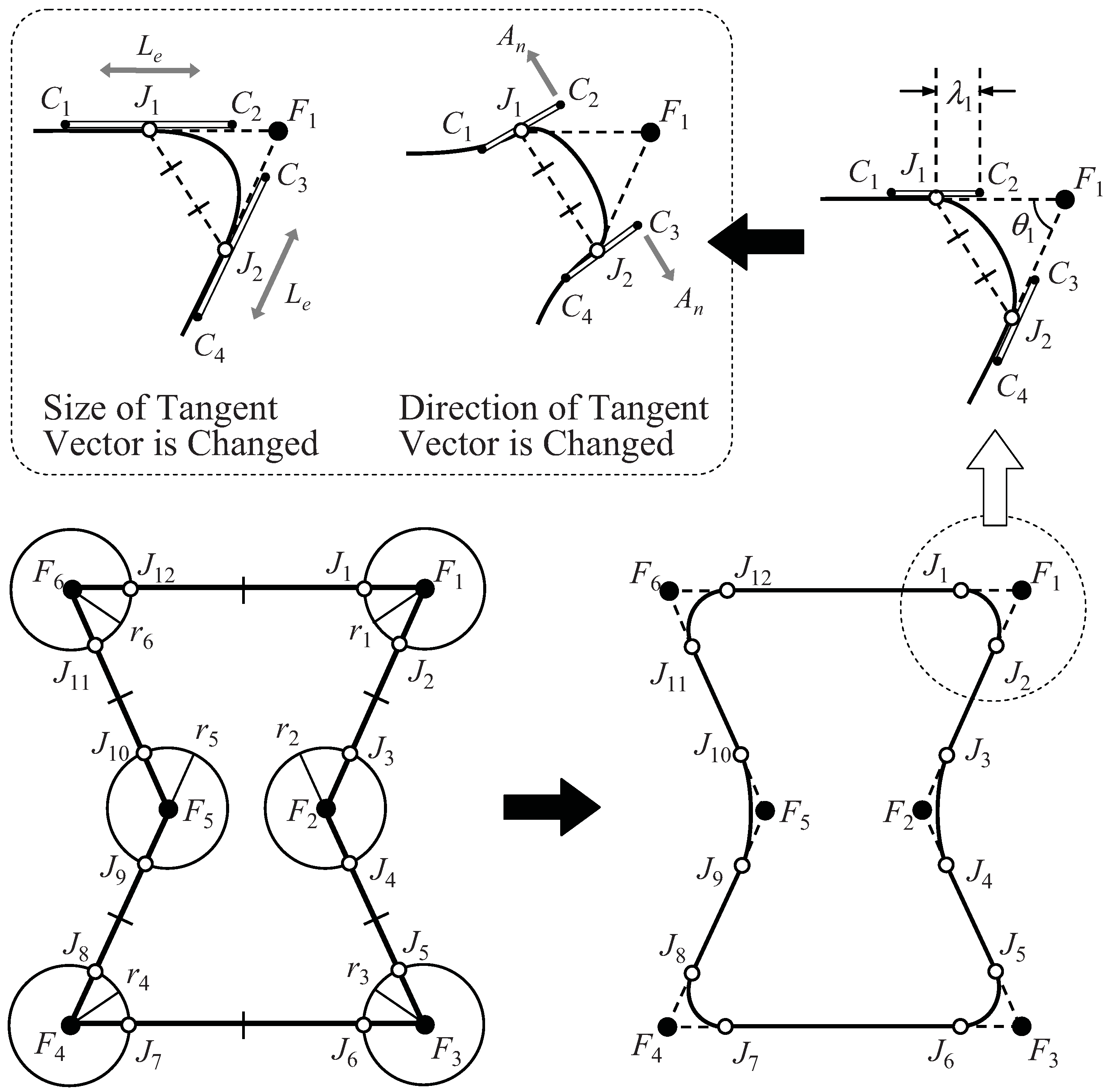
- (3)
- Angle of a tangent vector:nreal is used as the ratio for the movable range of the angle (i.e., an angle of the tangent vector is calculated as the product of the range and nreal).
- (4)
- Size of a tangent vector:nreal is used as the ratio for the movable range of the size (i.e., a size of the tangent vector is calculated as the product of the range and nreal).


6. Application of Shape Generation Method
6.1. Description of the Initial Shape and Conditions in the Genetic Algorithm


6.2. Shape Generation and Cognition Experiment
- (1)
- Method: semantic differential method (5 stages)
- (2)
- Samples: generated shapes (10 samples for each condition-type of macroscopic shape information, w, and ΔH)
- (3)
- Evaluation item: “complex”
- (4)
- Examinees: 13 students in their early 20 s
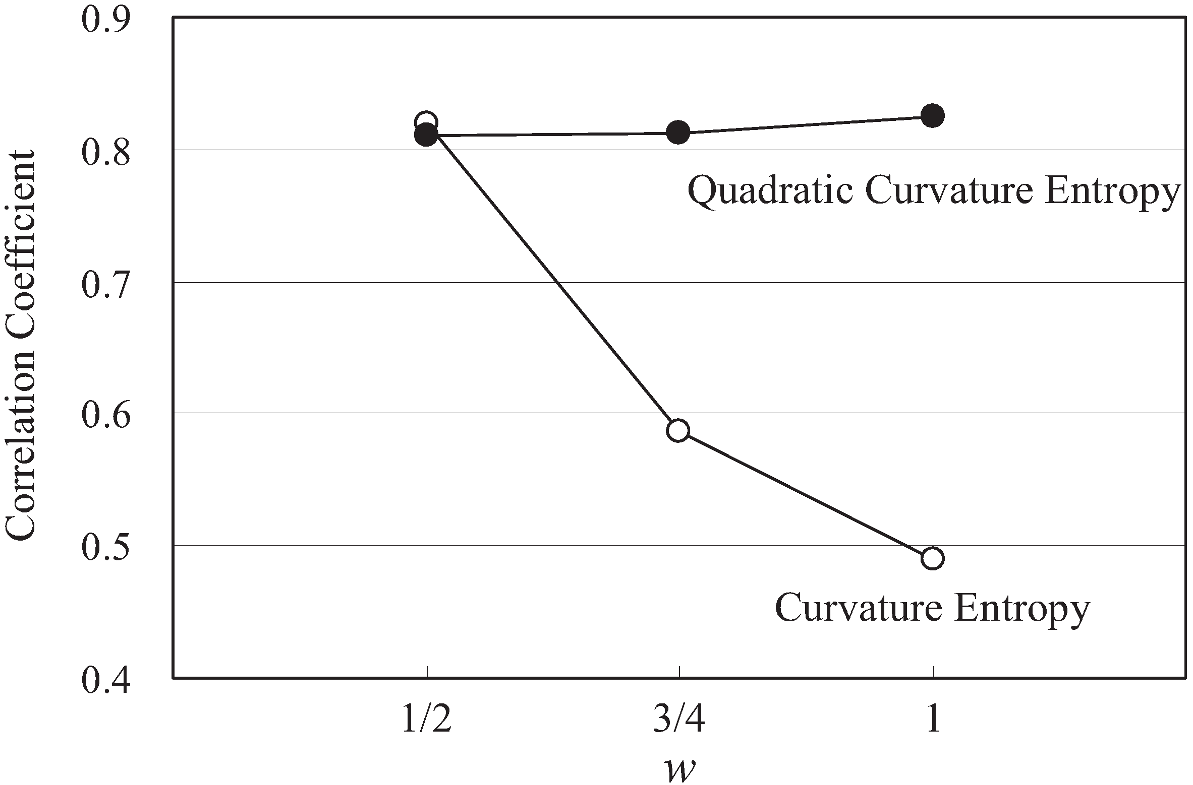
6.3. Relationship between Macroscopic Shape Information and Cognition Information
7. Conclusions
- (1)
- Validating the method constructed in this study for other shapes such as natural/geometric shapes and not just basic curved profiles.
- (2)
- Evaluating the relationship between the cognition of the complexity and scale dealt with in the field of CSS (Curvature Schale Space).
- (3)
- Comparing the genetic algorithm to other methods that search for curved profiles by changing the curved control variables.
Acknowledgments
References and Notes
- Metzger, W. Gesetze des Sehens, 2nd ed.; Kramer: Frankfurt, Germany, 1953. [Google Scholar]
- Beck, J. Effect of orientation and of shape similarity on perceptual grouping. Percept. Psychophys. 1966, 1, 300–302. [Google Scholar] [Green Version]
- Beck, J. Perceptual grouping produced by changes in orientation and shape. Science 1966, 154, 538–540. [Google Scholar] [CrossRef] [PubMed]
- Polanyi, M. The Tacit Dimension; Routledge & Kegan Paul Ltd.: London, UK, 1966. [Google Scholar]
- Kanizsa, G. Subjective contours. Sci. Am. 1976, 234, 48–52. [Google Scholar] [CrossRef] [PubMed]
- Kuyama, H. Measurements of feature-parameters of signs. Science of Design 1998, 45, 35–44. [Google Scholar]
- Asada, H.; Brady, M. The curvature primal sketch. IEEE Trans. Pattern. Anal. Mach. Intell. 1986, 8, 2–14. [Google Scholar] [CrossRef] [PubMed]
- Mokhtarian, F.; Mackworth, A.K. Scale-based description and recognition of planar curves and two-dimensional shapes. IEEE Trans. Pattern. Anal. Mach. Intell. 1986, 8, 34–43. [Google Scholar] [CrossRef] [PubMed]
- Mokhtarian, F.; Mackworth, A.K. A theory of multiscale, curvature-based shape representation for planar curves. IEEE Trans. Pattern. Anal. Mach. Intell. 1992, 14, 789–805. [Google Scholar] [CrossRef]
- Mokhtarian, F. Silhouette-based isolated object recognition through curvature scale space. IEEE Trans. Pattern. Anal. Mach. Intell. 1995, 17, 539–544. [Google Scholar] [CrossRef]
- Harada, T.; Yoshimoto, F.; Moriyama, M. An aesthetic curve in the field of industrial design. In Proceedings of the 1999 IEEE Symposium on Visual Language, Tokyo, Japan, 13–16 September 1999; pp. 38–47.
- Harada, T.; Mori, N.; Sugiyama, K. Study of quantitative analysis of curve’s character. Science of Design 1994, 40, 9–16. [Google Scholar]
- Harada, T.; Mori, N.; Sugiyama, K. Algorithm of creating the curve by controlling its characteristics. Science of Design 1994, 41, 1–8. [Google Scholar]
- Jernigan, M. E.; D'Astous, F. Entorpy based texture analysis in the spatial frequency domain. IEEE Trans. Pattern. Anal. Mach. Intell. 1984, 6, 237–243. [Google Scholar] [CrossRef] [PubMed]
- Thiran, P.; Crounse, R.K.; Chua, O.L.; Hasler, M. Pattern formation properties of autonomous cellular neural networks. IEEE Trans. Circuits. Syst. I 1995, 42, 757–774. [Google Scholar] [CrossRef]
- Ujiie, Y.; Matsuoka, Y. Shape-generation method using curvature entropy. In Proceedings of the 2000 ASME International Mechanical Engineering Congress and Exposition, Orlando, FL, USA, 5–10 November 2000; pp. 85–92.
- Shannon, C.E.; Weaver, W. The Mathematical Theory of Communication; The University of Illinois Press: Chicago, IL, USA, 1964. [Google Scholar]
- Blahut, R.E. Principles and Practice of Information Theory; Addison-Wesley Publishing Company: Boston, MA, USA, 1987. [Google Scholar]
- Ujiie, Y.; Matsuoka, Y. Macro-informatics of cognition and its application for design. Adv. Eng. Informat. 2009, 23, 184–190. [Google Scholar] [CrossRef]
- Birkhoff, G.D. Aesthetic Measure; Harvard University Press: Cambridge, UK, 1933. [Google Scholar]
- Miura, M.; Sugihara, T.; Kunifuji, S. GKJ: Group KJ method support system utilizing digital pens. IEICE Trans. Info. Syst. 2011, E94-D, 456–464. [Google Scholar] [CrossRef]
- Hosaka, M. Modeling of Curves and Surfaces in CAD/CAM; Springer-Verlag: Berlin, Germany, 1992. [Google Scholar]
- Yamaguchi, F. Curves and Surfaces in Computer Aided Geometric Design; Springer-Verlag: Berlin and Heidelberg, Germany, 1988. [Google Scholar]
- Suzuki, T.; Asanuma, T.; Matsuoka, Y. The proposal of the macroscopic design information as a shape design index. In Proceedings of the 4th Asian Design Conference, Nagaoka, Niigata, Japan, 30–31 October 1999; pp. 214–221.
- Tian, M.; Sugiyama, K.; Kamaike, M.; Watanabe, M. A car form generation system based on evolutionary computation. Science of Design 1997, 44, 77–86. [Google Scholar]
- Tian, M.; Sugiyama, K.; Kamaike, M.; Watanabe, M.; John, S. A design support system based on co-evolutionary process. Science of Design 1998, 45, 65–74. [Google Scholar]
- Obayashi, S. Aerodynamic design and inverse problem. Science of Design 1996, 1, 21–27. [Google Scholar]
© 2012 by the authors. Licensee MDPI, Basel, Switzerland. This article is an open access article distributed under the terms and conditions of the Creative Commons Attribution license ( http://creativecommons.org/licenses/by/3.0/).
Share and Cite
Ujiie, Y.; Kato, T.; Sato, K.; Matsuoka, Y. Curvature Entropy for Curved Profile Generation. Entropy 2012, 14, 533-558. https://doi.org/10.3390/e14030533
Ujiie Y, Kato T, Sato K, Matsuoka Y. Curvature Entropy for Curved Profile Generation. Entropy. 2012; 14(3):533-558. https://doi.org/10.3390/e14030533
Chicago/Turabian StyleUjiie, Yoshiki, Takeo Kato, Koichiro Sato, and Yoshiyuki Matsuoka. 2012. "Curvature Entropy for Curved Profile Generation" Entropy 14, no. 3: 533-558. https://doi.org/10.3390/e14030533
APA StyleUjiie, Y., Kato, T., Sato, K., & Matsuoka, Y. (2012). Curvature Entropy for Curved Profile Generation. Entropy, 14(3), 533-558. https://doi.org/10.3390/e14030533