Tsallis-Based Nonextensive Analysis of the Southern California Seismicity

Abstract

Nonextensive statistics has been becoming a very useful tool to describe the complexity of dynamic systems. Recently, analysis of the magnitude distribution of earthquakes has been increasingly used in the context of nonextensivity. In the present paper, the nonextensive analysis of the southern California earthquake catalog was performed. The results show that the nonextensivity parameter q lies in the same range as obtained for other different seismic areas, thus suggesting a sort of universal character in the nonextensive interpretation of seismicity.

1. Introduction

The cumulative number of earthquakes with magnitude m > M_th is log-linearly related with the threshold magnitude M_th by the well known Gutenberg-Richter (GR) law [1]. In terms of energy, this empirical relationship represented one of the features characterizing the self-organizing criticality due to the power-law dependence of the cumulative number of earthquakes with energy [2]. Although this relationship is very important, because it explains from a statistical viewpoint the seismicity occurring in seismic regions, it was not related with general physical principles apart from a recent attempt [3] in which the GR law seems to result from the Maximum Entropy Principle when considering the natural time concept [4], which, among others, allows the determination of an impending mainshock [3] when analyzing in natural time the seismicity that occurs after the recording of a Seismic Electric Signals activity [5,6].

Sotolongo-Costa and Posadas [7] developed an intriguing model for earthquake generation mechanism, which starting from first principles led to an energy distribution function, including the GR law as a particular case. In this model the fragments between the irregularities of the fault planes, originated by the local breakage of the tectonic plates, from which the faults are generated interact. The result of this interaction are earthquakes. The use of the nonextensive Tsallis formalism [8] was, then, implied by the physical picture of such a model and a fragment size distribution was derived, which, combined with the roughness of the fault planes, leads to a mechanism of earthquake triggering. The Sotolongo-Costa and Posadas’ model was revisited by Silva et al. [9], who adopted a more realistic relationship between earthquake energy and fragment size, in full agreement with the standard theory of seismic moment scaling with rupture length [10]; as a consequence, a slightly different magnitude distribution was deduced, providing an excellent fit to seismicity generated in various seismic regions. This model was recently applied to regional seismicity, covering diverse geological faults, down to specific seismic zones [11,12,13,14].

2. Nonextensivity in Modeling Earthquakes

Nonextensivity represents one of the most intriguing characteristics of systems that experience long-range spatial correlations or long-range memory effects. In nonextensive systems the Boltzmann-Gibbs (BG) statistics, in which the entropy is additive and includes just short-length interactions so that the total entropy depends on the size of the object, is violated. Tsallis [8] generalized the BG statistics, introducing an entropic expression parameterized by q, which measures the degree of nonextensivity; as a particular case, the extensive BG statistics is recovered by q = 1. Contrarily to the BG statistics, the Tsallis’ nonextensive formulation of entropy allows all-length scale interactions. The process of shock fragmentation, especially when high energies are involved, leads to the existence of long-range interactions between all parts of the object being fragmented, and this type of entropy is nonadditive and depends on the object as a whole. Thus, the use of the nonextensive approach seems adequate to analyze the complex mechanism of relative displacement of fault plates interacting with the fragments between them.

The model, as developed by Silva et al. [9], assumes that the eventual relative position of fragments filling the space between two irregular faults can hinder their relative motion. Stress increases until a displacement of one of the asperities, due to the displacement of the hindering fragment, or even its breakage in the point of contact with the fragment leads to a relative displacement of the fault planes of the order of the size ρ of the hindering fragment, with the subsequent energy release ε [7]. 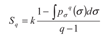Since large fragments are more difficult to release than small ones, this energy ε~ρ³, in agreement with the scaling relationship between seismic moment and rupture length [10]. The maximum entropy principle for the Tsallis’ entropy [8] is given by:

(1)

where p_σ (σ) is the probability of finding a fragment of surface σ and q is a real number; k is the Boltzaman constant. It is easy to see that this entropy is the Boltzmann entropy when q→1. Let’s set k = 1 for sake of simplicity.

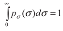
The probability p_σ (σ) is obtained maximizing the Tsallis’ entropy under the two constraints:

(1) the normalization of p_σ (σ):

(2)

(2) the condition about the q-expectation value [15]:

(3)

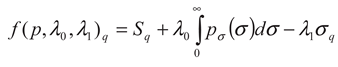
For q→1, the last condition becomes the definition of mean value. Using the technique of Lagrange multipliers, the following functional is maximized:

(4)

where λ₀ and λ₁ are the Lagrange multipliers. Imposing that:

(5)

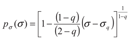
After some algebra, the area distribution for fragments of the fault planes is obtained [9]:

(6)

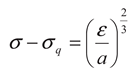
Assuming the energy scale ε~ρ³, the proportionality between the released energy ε and ρ³ becomes:

(7)

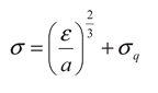
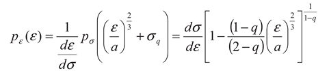
where σ scales with ρ² and a (the proportionality constant between ε and ρ³) is proportional to volumetric energy density. Thus, the energy distribution function (EDF) of the earthquakes is obtained in the following manner: using the transformation given by Equation 5, the variable σ is derived as:

(8)

On the base of the relationship between density functions of correlated stochastic variables [16], the EDF is given by:

(9)

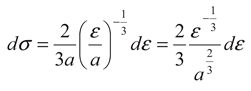
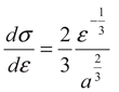
By differentiating Equation 6:

(10)

from which:

(11)

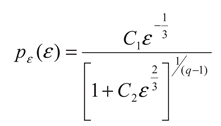
The EDF is now given by:

(12)

with

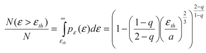
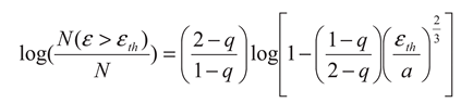
The probability of energy p_ε(ε) = n(ε)/N, where n(ε) is the number of earthquakes of energy ε and N the total number of earthquakes. The normalized cumulative number of earthquakes can be obtained by integrating Equation (10):

(13)

where N(ε > ε_th) is the number of earthquakes with energy larger than the threshold ε_th, and thus:

(14)

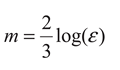
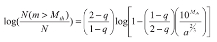
Substituting in Equation (12) the relationship:

(15)

where m is the magnitude, the distribution of the number N of earthquakes with magnitude m larger than the threshold M_th normalized to the total number of events is given by:

(16)

These results incorporate the characteristics of nonextensivity into the distribution of earthquakes by magnitude. Equation 14 is slightly different from that obtained by Silva et al. [9], who used the relation m = log(ε)/3.

3. Application to the Southern California Earthquake Catalog

In the present study the earthquakes occurred during year 2010 in Southern California were investigated. The earthquakes were extracted from the SCEDC (Southern California Earthquake Data Center) seismic catalogue [17]. Only shallow earthquakes (depth 0–60 km) were investigated.

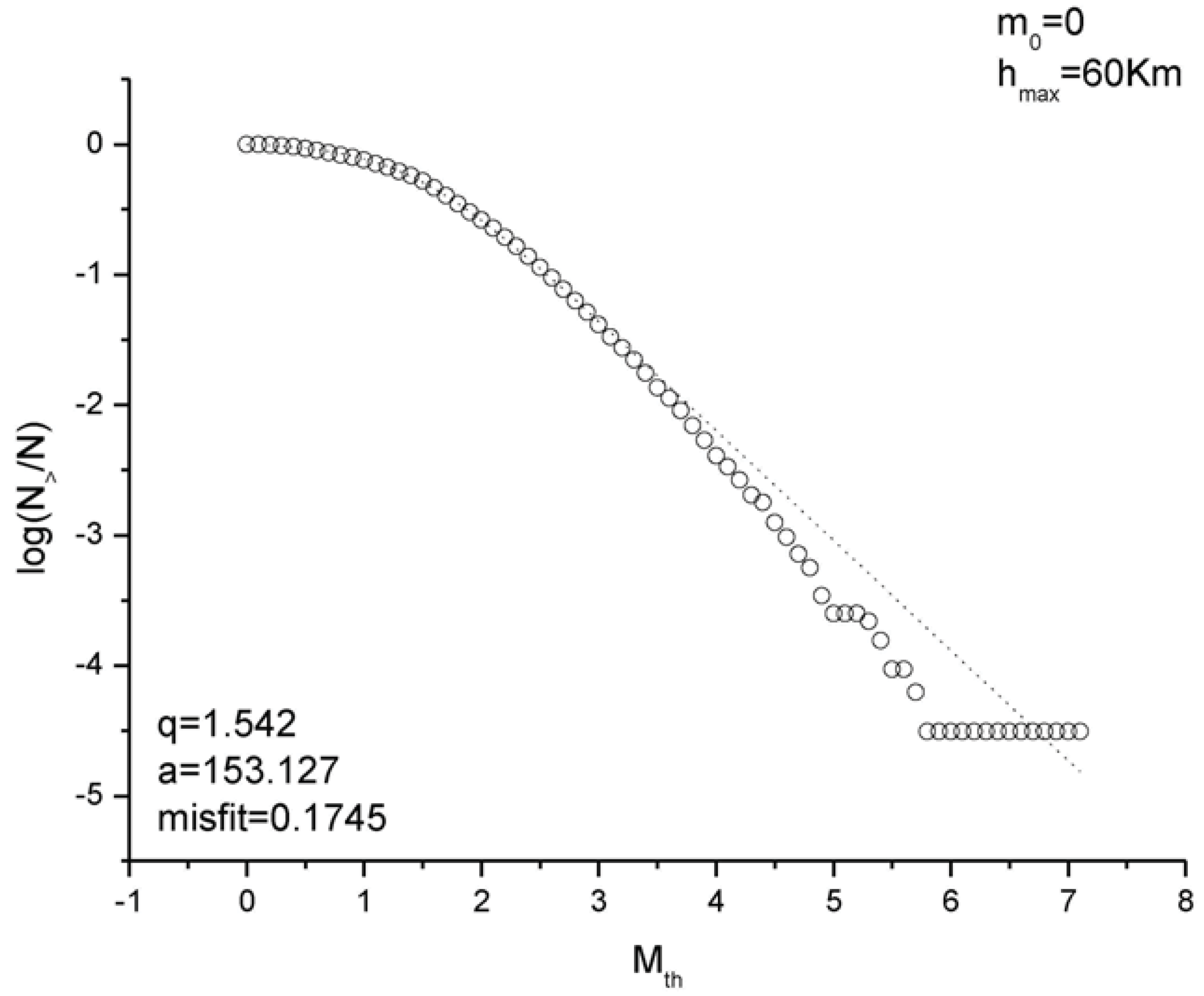
Figure 1 shows the distribution of the relative number of earthquakes with magnitude m > M_th for minimum threshold magnitude m₀ = 0 and maximum depth h_max = 60 km. The curve fitting the data and representing Equation (16) has nonextensive parameters q = 1.542 and a = 153.127 estimated by the maximum likelihood estimation (MLE) method [18]. The misfit was evaluated by means of the average of the absolute values of the residuals |y-y_fit|, where y indicates the real value and y_fit the predicted value by the fitting. For m₀ = 0 the misfit is about 0.1745. The deviation of the fitting curve from the normalized cumulative distribution function at large magnitudes is due to the almost constant value of the distribution within the range of magnitudes from 5.8 to 7.2.

Figure 1. Magnitude distribution and fitting with Equation 16 for the whole catalog (depth less than 60 km and minimum magnitude m₀ = 0). The black continuous line indicates the nonextensive fitting curve.

Figure 1. Magnitude distribution and fitting with Equation 16 for the whole catalog (depth less than 60 km and minimum magnitude m₀ = 0). The black continuous line indicates the nonextensive fitting curve.

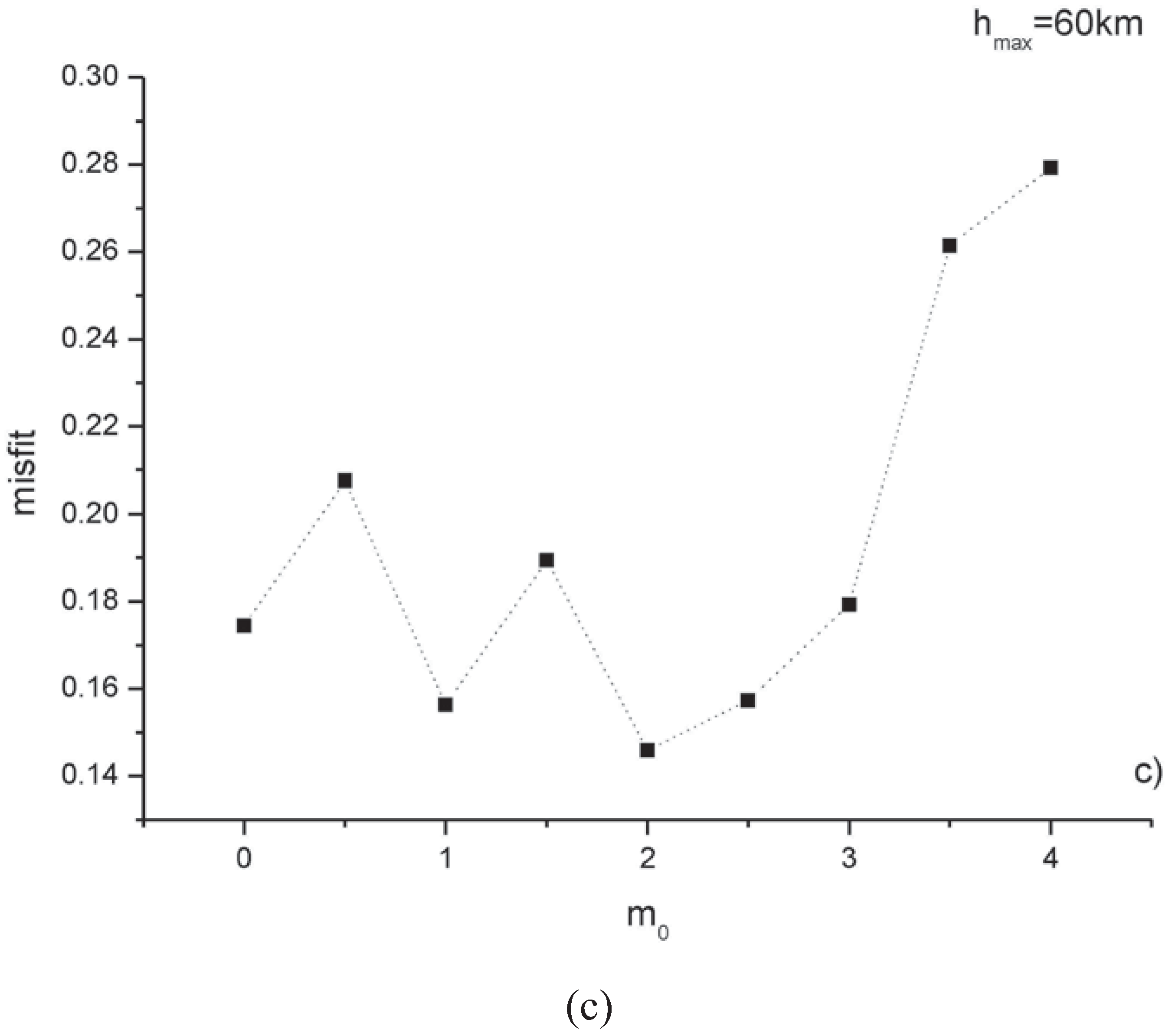
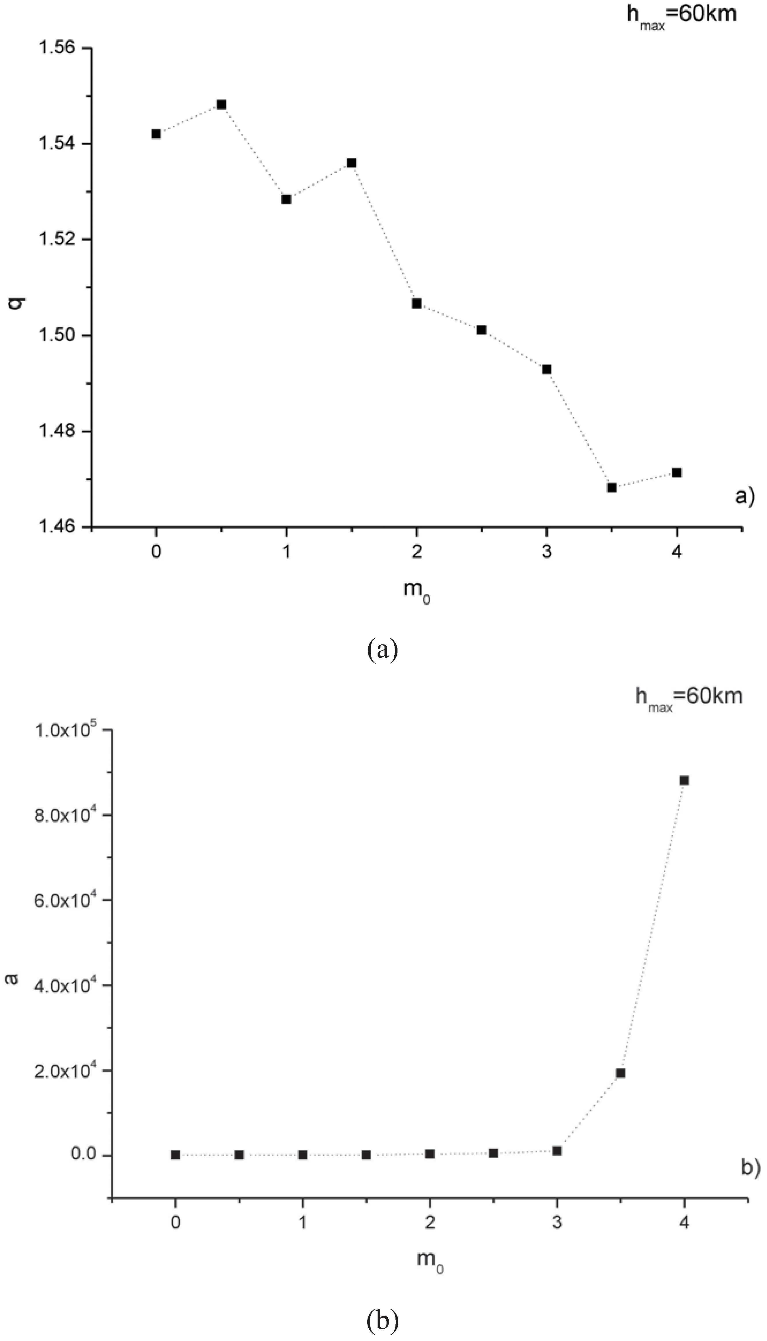
Figure 2 shows the variation with the minimum magnitude m₀ of the nonextensive parameters q and a and the misfit. The dependence of the parameters with the minimum magnitude, revealing that q approximately decreases with m₀, while a increases, is visible. However, the best model is for the minimum magnitude m₀ to which corresponds the values of q = 1.506 and a = 438.65 (misfit = 0.146).

Figure 2. Variation with the minimum magnitude m₀ of q (a), a (b), and misfit (c), for maximum depth h_max = 60 km. The best nonextensive model for the catalogue is for m₀ = 2.0 (q = 1.506, a = 438.65).

Figure 2. Variation with the minimum magnitude m₀ of q (a), a (b), and misfit (c), for maximum depth h_max = 60 km. The best nonextensive model for the catalogue is for m₀ = 2.0 (q = 1.506, a = 438.65).

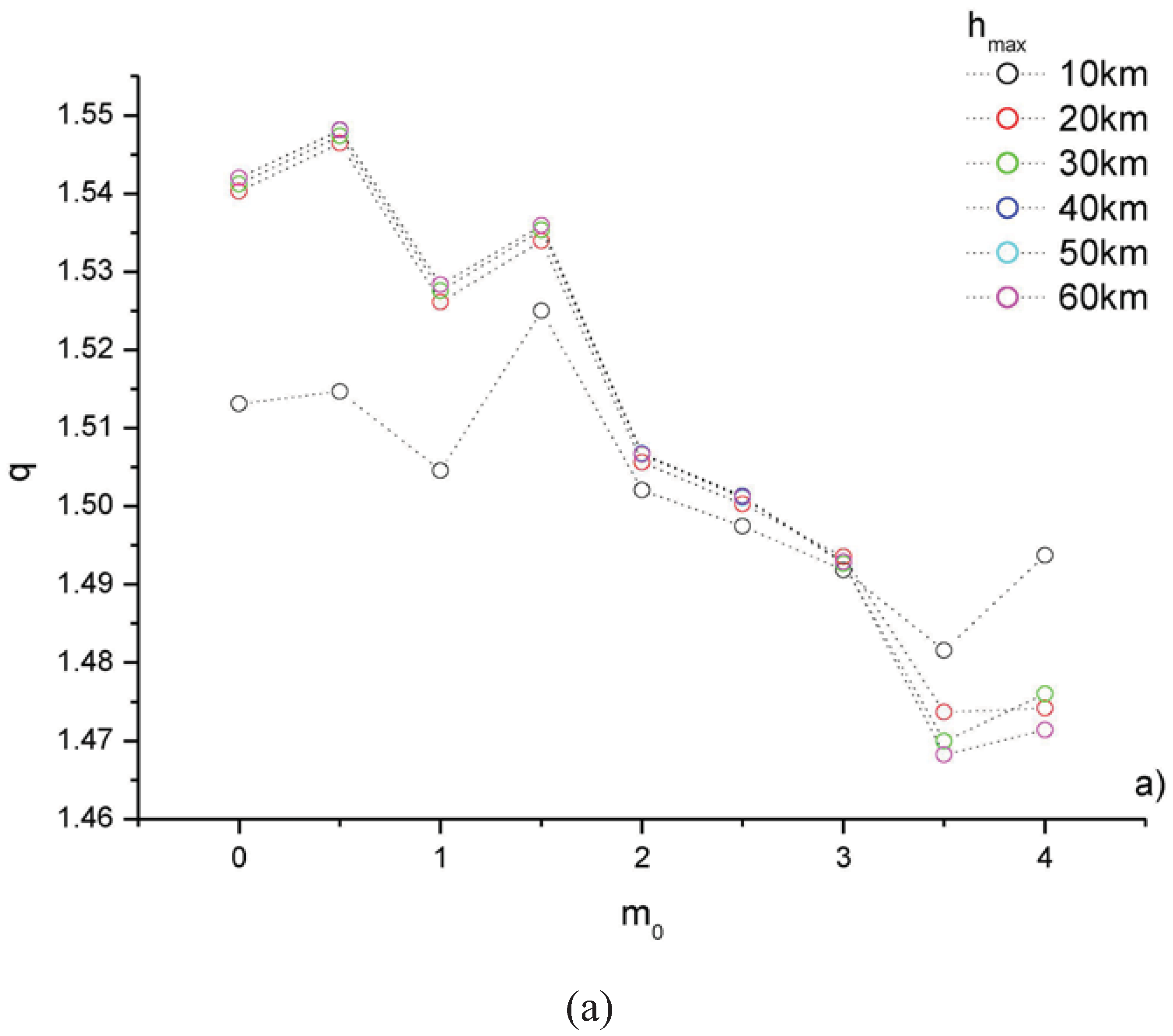
Figure 3 shows the variation with m₀ and h_max of q, a and the misfit. It is clearly visible that all the curves are almost identical, except for that corresponding to h_max = 10 km.

Figure 3. Variation with the minimum magnitude m₀ and h_max of q (a), a (b), and misfit (c).

Figure 3. Variation with the minimum magnitude m₀ and h_max of q (a), a (b), and misfit (c).

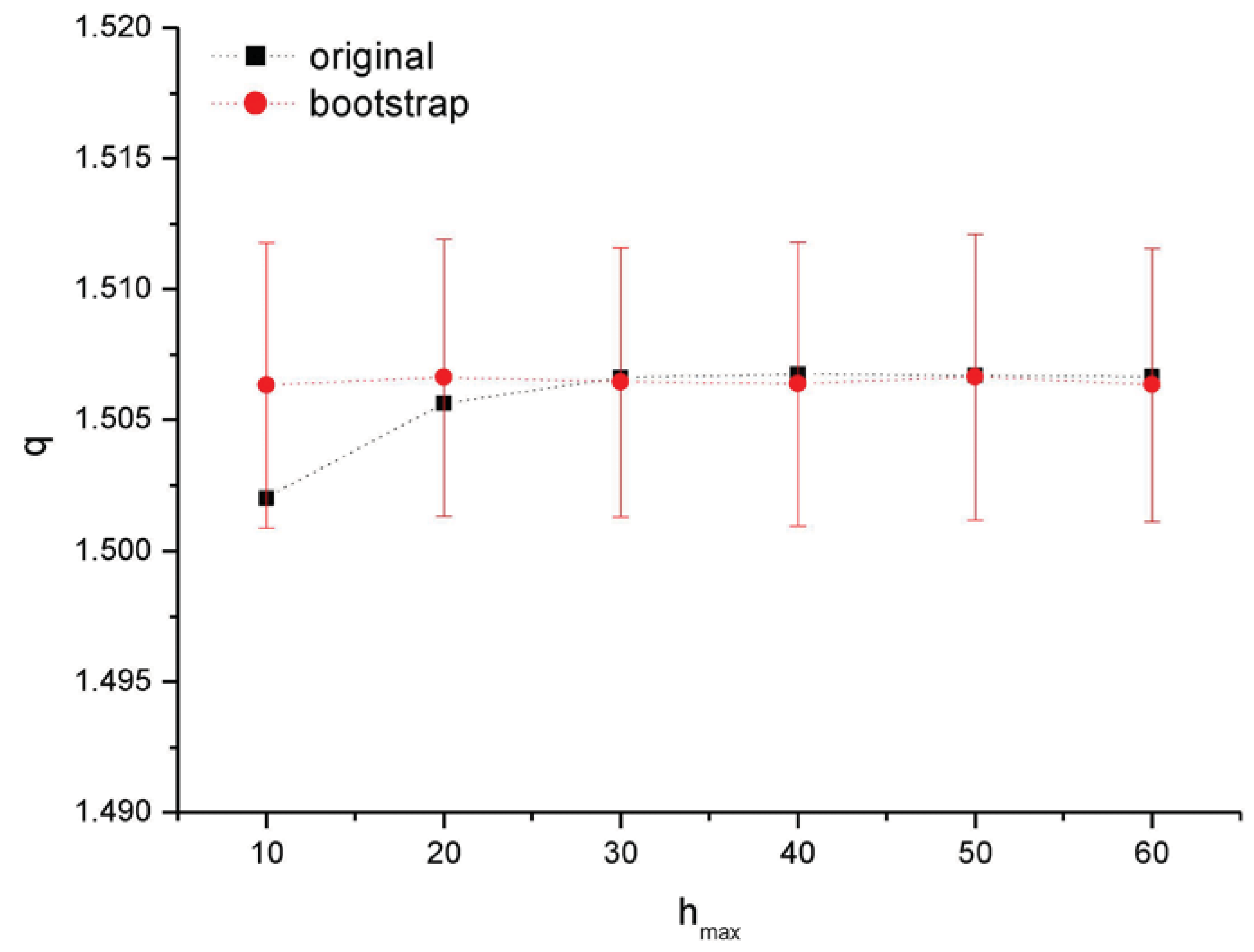
In order to assess the accuracy of the estimated nonextensive parameters, the following procedure was performed. The minimum magnitude m₀ = 2.0 was fixed (which corresponded to the best nonextensive model) and one thousand magnitude sequences were simulated by means of the bootstrap method [19] for any value of the maximum depth h_max from 10 km to 60 km. For any of these simulated sequence the nonextensive parameters q_S and a_S were estimated applying the MLE. Then the mean and standard deviation of q_S and a_S were calculated. Figure 4 and Figure 5 show the variation of mean and standard deviation of the nonextensive parameters of q_S and a_S varying the maximum depth h_max. It is clearly shown that the nonextensive parameters estimated for the original series are quasi identical with the average q_S and a_S and the small standard deviation indicates a very good accuracy of the estimates.

Figure 4. Results of the application of the bootstrap method with varying the maximum depth h_max (m₀ = 2.0). The black squares represent the variation of the q value of the original magnitude sequence; the red circles (bars) are the mean (standard deviation) of the q_S.

Figure 4. Results of the application of the bootstrap method with varying the maximum depth h_max (m₀ = 2.0). The black squares represent the variation of the q value of the original magnitude sequence; the red circles (bars) are the mean (standard deviation) of the q_S.

Figure 5. Results of the application of the bootstrap method with varying the minimum depth h_max (m₀ = 2.0). The black squares represent the variation of the a value of the original magnitude sequence; the red circles (bars) are the mean (standard deviation) of the a_S.

Figure 5. Results of the application of the bootstrap method with varying the minimum depth h_max (m₀ = 2.0). The black squares represent the variation of the a value of the original magnitude sequence; the red circles (bars) are the mean (standard deviation) of the a_S.

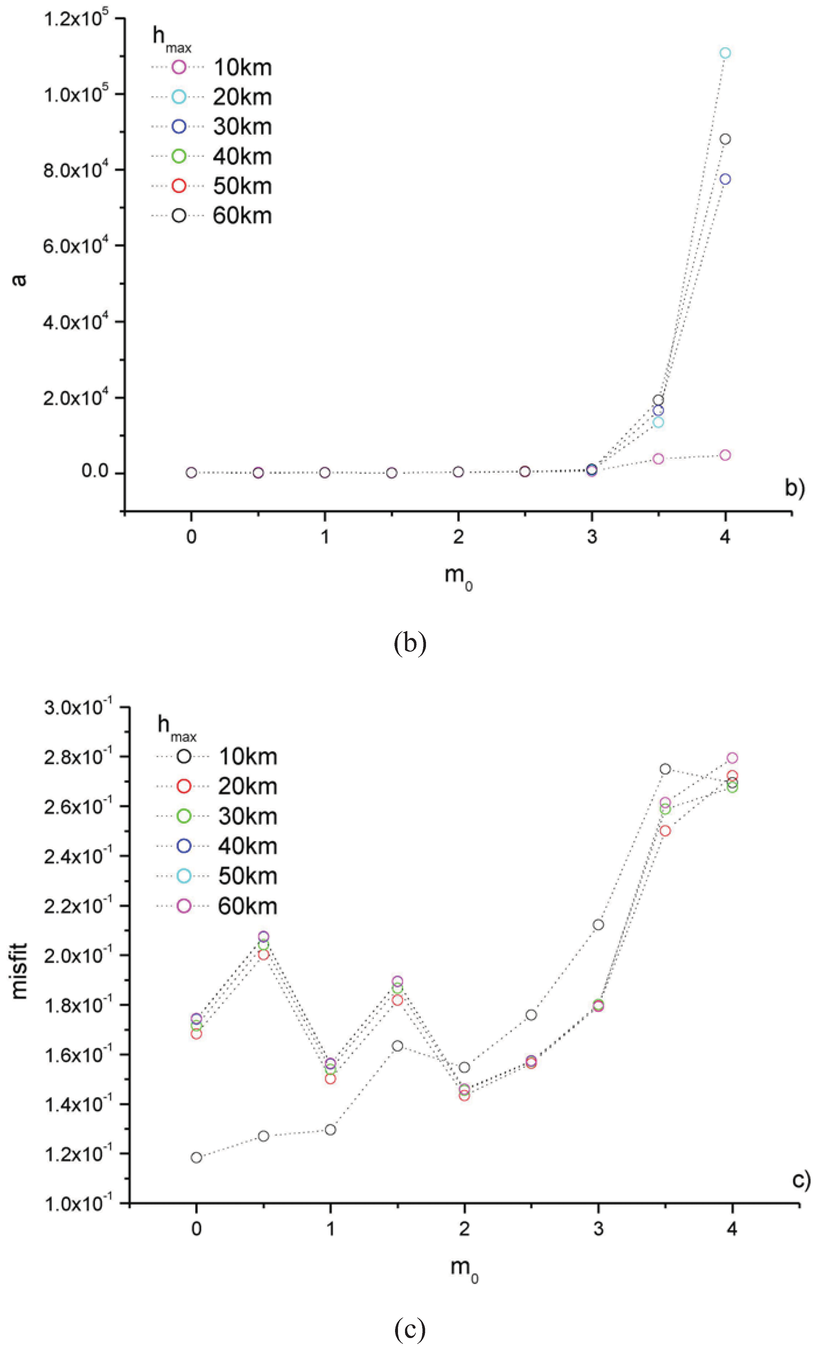
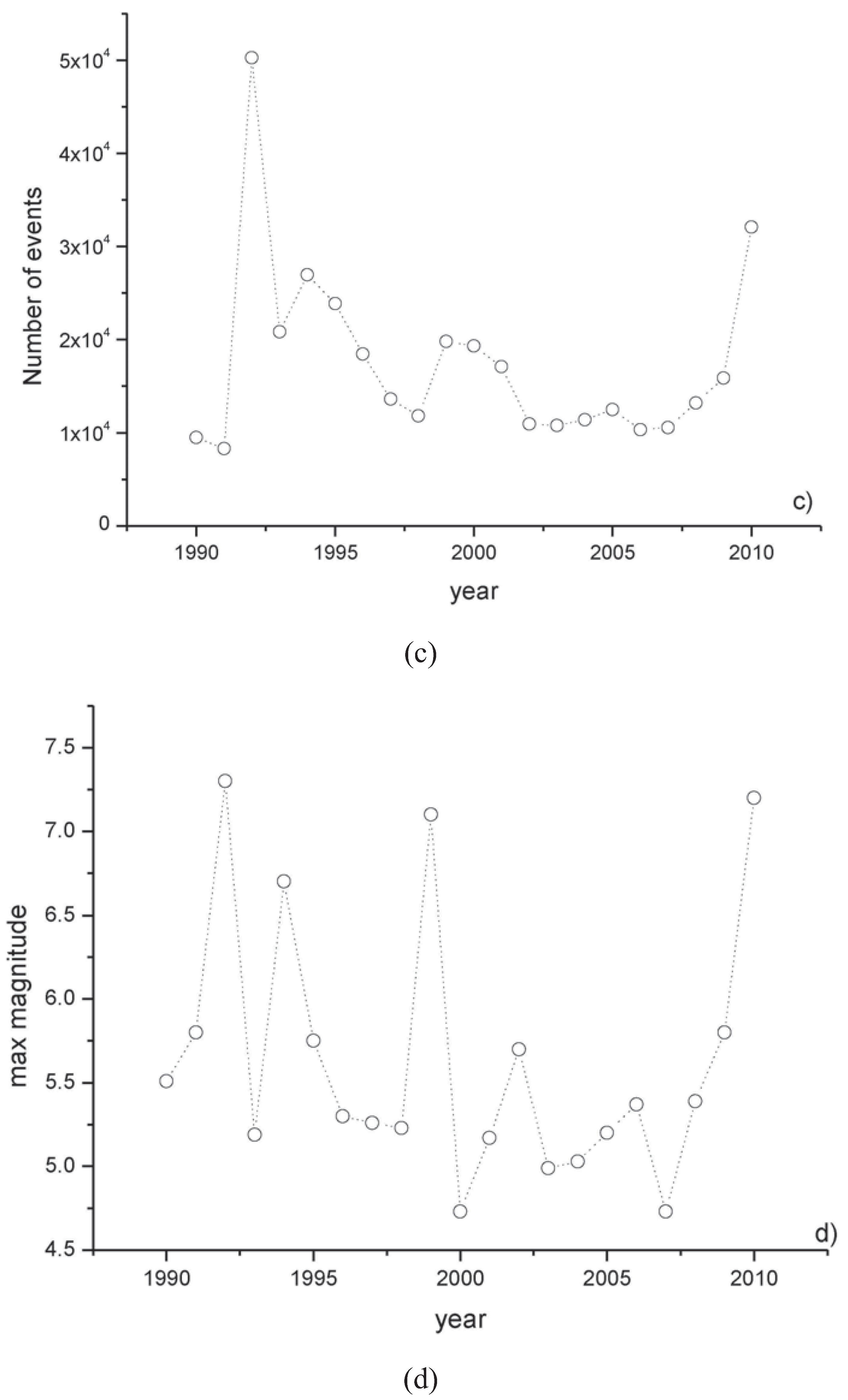
The time variation of the nonextensive parameters was analyzed. The yearly values of q and a were calculated for the seismicity of the southern California from 1990 to 2010 (Figure 6). It is visibly clear that the q-value is almost constant up to 2004, then it increases up to 2010. The a-value is characterized by two significant spikes in 1992 and 1999, while it ranges between 100 and 250 up to 2003, and around a lower value (~50) from 2004 to 2009. Figure 6 shows also the yearly variation of the number of events and the maximum magnitude.

Figure 6. Yearly variation of the q (a), a (b), number of events (c) and maximal magnitude (d) for the seismicity of Southern California.

Figure 6. Yearly variation of the q (a), a (b), number of events (c) and maximal magnitude (d) for the seismicity of Southern California.

4. Discussion

The decrease (increase) of q (a) with the minimum magnitude m₀ is not an easy task. In the context of the fragment-asperity model, the nonextensivity parameter q quantifies the scale of spatial interactions: for q~1, the spatial correlations are short-ranged and physical state is in quasi-equilibrium. For increasing q, the physical state goes away from equilibrium; and in case of seismicity, this means that the fault planes and fragment filling the gap between them are not in equilibrium, leading to an increased seismic activity to be expected [12]. In [20] the decrease of the nonextensivity parameter q was observed during relatively quiet periods, characterized mainly by the occurrence of small magnitude events; this could reveal that the order within the system of fault is decreased and the amount of accumulated stress is not yet enough to initiate a correlated behavior of the whole system [21]. When a strong earthquake occurs, more correlated behavior of the system constituents is assumed to take place, with the emergence of short and long range correlations, which induce an increase of the nonextensivity parameter q.

In the case examined in the present paper, we observe a decrease of the parameter q with the increase of the minimum magnitude. Probably the main reason of such decreasing trend could be the decreased number of small events, which are removed by choosing a higher magnitude threshold. Removing all the smaller events, also the possible interactions and correlations, which can take place with a higher probability when many small events are considered, are reduced, leading the whole system to a quasi-equilibrium-like status. Therefore, the smaller events seem to be necessary for an earthquake system to redistribute the stress in order to initiate a status where correlations and interactions can take place also among higher events. It seems that the smaller events behave as links among the higher events, where the correlations are transferred, thus producing an enhancement of the q-value.

The increase of the a-value can just be due the larger energy released by higher events.

The time variation of the nonextensivity parameters shows the following effects:

(i)

a takes the highest values during years in which the events with highest magnitude occurred; a is the volumetric energy density, and its value is large if the energy released is large.

(ii)

from 2004 to 2009, the increase of q is reflected by a slight decrease of a; during this period of reduced seismic activity (indicated by a reduced number of events) and without very large earthquakes (indicated by a maximal magnitude ranging between 4.5 and 5.5), the volumetric energy density is reduced, the accumulated stress energy seems to be released mostly through the relative movement of smaller fragments, but the increased degree of the system interactions are mainly governed by the smaller events.

5. Conclusions

The SCEDC catalog was analyzed by means of a nonextensive approach, which takes into account not only the overlapping of irregular profiles of fault planes but also the hindering fragments generated by the breakage of the faults. The analysis of the variation of the nonextensive parameters a and q was performed varying the minimum threshold moment magnitude (from 0 to 4.0) and the maximum hypocentral depth (from 10 km to 60 km). The smallest value of the misfit between the real and the fitted distribution was for minimum threshold magnitude 2.0. The time variation of q appears quite stable from 1990 to 2004, but shows an increasing trend from 2005 to 2010. The time variation of a reveals two anomalous values in 1992 and 1999. The present study confirms that the non-additive parameter q can be considered for a unique description of seismicity.