Abstract
Some problems occurring in Expert Systems can be resolved by employing a causal (Bayesian) network and methodologies exist for this purpose. These require data in a specific form and make assumptions about the independence relationships involved. Methodologies using Maximum Entropy (ME) are free from these conditions and have the potential to be used in a wider context including systems consisting of given sets of linear and independence constraints, subject to consistency and convergence. ME can also be used to validate results from the causal network methodologies. Three ME methods for determining the prior probability distribution of causal network systems are considered. The first method is Sequential Maximum Entropy in which the computation of a progression of local distributions leads to the over-all distribution. This is followed by development of the Method of Tribus. The development takes the form of an algorithm that includes the handling of explicit independence constraints. These fall into two groups those relating parents of vertices, and those deduced from triangulation of the remaining graph. The third method involves a variation in the part of that algorithm which handles independence constraints. Evidence is presented that this adaptation only requires the linear constraints and the parental independence constraints to emulate the second method in a substantial class of examples.
1. Introduction
In Expert Systems the Maximum Entropy (ME) methodology [1,2,3] can be employed to augment that of Causal Networks (CNs), e.g., HUGIN [4] and Lauritzen-Spiegelhalter [5]; also see Neapolitan [3]. The philosophy and motivation for using ME has already been examined in earlier work, see [6,7,8,9,10] and [11]. ME provides a parallel methodology which can be used to validate results from the CNs methodologies and there is also the potential for application beyond the strict limits of CNs. The work here will be confined to binary variables (true or false), the aim being to deduce prior probability distributions (solutions) which exhibit maximal entropy and match outcomes from CNs when appropriate. Three methods to this effect will be presented.
A causal network relates propositional variables and has the following properties: a prior probability is required for each root (a source node with no edges directed into it) and a set of prior conditional probabilities must be available at every other vertex giving the probability of the associated variable for all assignments to the variables representing its parents. These probabilities constitute the linear constraints and such networks will be described as complete. The system is represented by a directed acyclic graph (DAG) and a set of independence constraints is implied. The discussion in the paper will focus on complete causal networks (Note that incomplete systems may exhibit multiple solutions, see Paris [12]. Some confusion exists regarding the appropriate terminology, quoting Neapolitan: “Causal networks are also called Bayesian networks, belief networks and sometimes influence diagrams” [3]. The first of these terms will be used throughout.
Independence constraints will be an important element of this paper (discussion of the Independence concept can be found in [13,14]) and the terminology to be used will now be clarified:
Absolute and conditional independence constraints between propositional variables will be represented, respectively, by forms such as:
The term independency will be used to identify the set of individual independence constraints generated by the possible assignments to the conditioning set.
For example, the generic independency will consist of four individual constraints:
Independencies between parents are formally termed moral independencies (moral graphs and also triangulation are discussed in [3], see also Figure 1, Figure 2, Figure 3 and Figure 4, and associated text. Moral independencies are conditioned by a set of variables blocking all ancestral paths between the parents. This set is empty in the case of absolute independence.
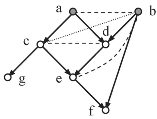
Figure 1.
Tree-Loz-Vee-Tri7.
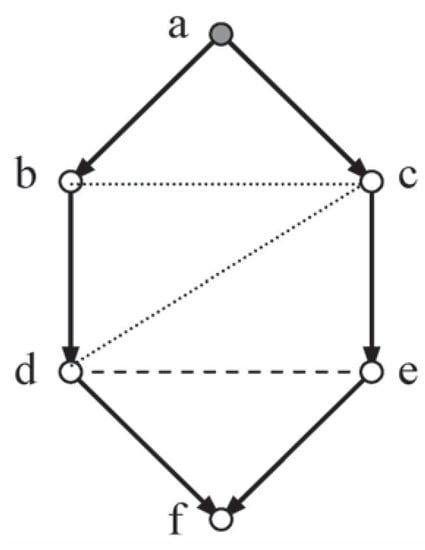
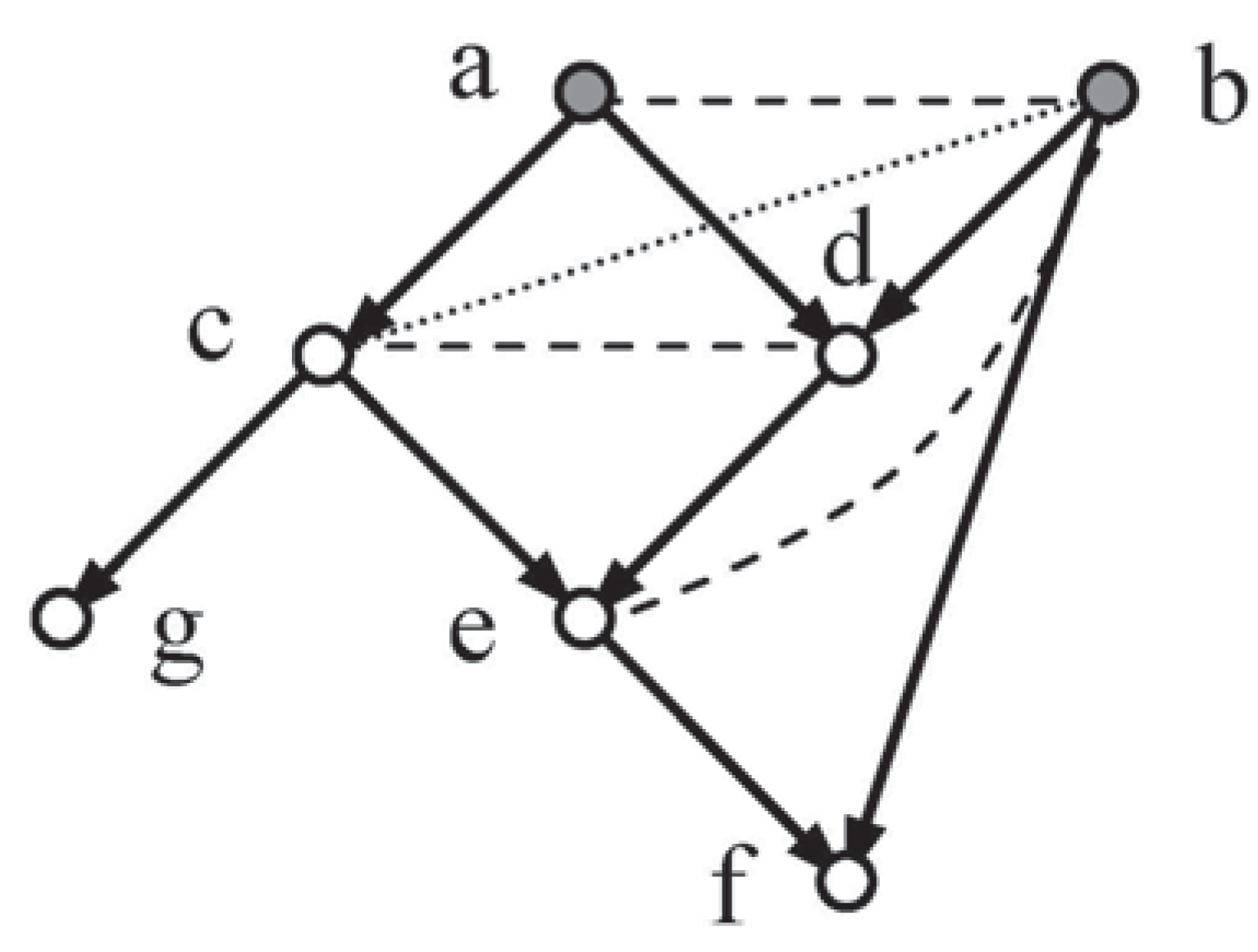
Figure 2.
Loz6.
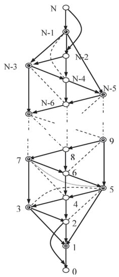
Figure 3.
Emb-LozN.
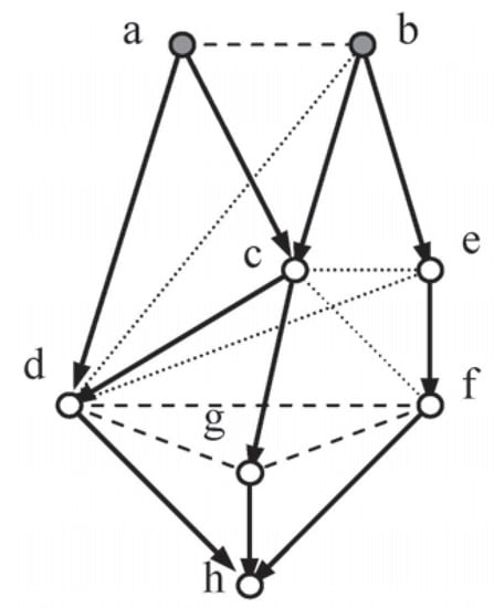
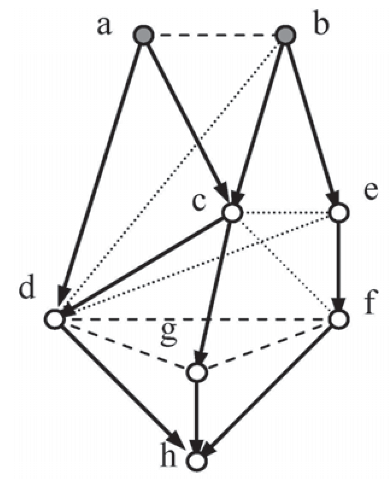
Figure 4.
Random-Test8.
With regard to the first method, Lukasiewicz has proved that the application of ME to a causal network produces a unique solution using Sequential ME [15]. This process will be exemplified in Section 1. An understanding of d-Separation is required and an explanation will be provided there.
ME methodologies based on the Method of Tribus [16] need an appropriate set of explicit independence constraints (void if only linear constraints are to be considered), and a technique for finding such a set is described in [17]. For the second method, both moral and triangulation independencies are required, in general. When these are in place the solution will match that from CNs [11]. The algorithm advanced handles consistent sets of linears and explicit independencies presented in a standard format.
The third method was suggested by a series of experimental results using a variation of the algorithm which requires just the linear constraints and the moral independencies. The handling of the independencies is accomplished by a technique based, initially, on the method developed for linears. This variant method will be applied to an elementary network, and then the technique developed will be extended to a more general system. Further generalisation of this method remains to be explored. This paper relates to an aspect of the work covered in my Ph.D. thesis successfully submitted to the University of Bradford in 2005 [11], under the supervision of P.C. Rhodes.
2. Method 1: Sequential Maximum Entropy (SME)
Quoting from the abstract to his paper, Lukasiewicz says:
“We thus present a new kind of maximum entropy model, which is computed sequentially. We then show that for all general Bayesian networks, the sequential maximum entropy model coincides with the unique joint distribution.”
The method uses d-Separation (d-sep) to determine local probabilities in descending order.
2.1. Definition of d-Separation
This is a mechanism for determining the implicit independencies of a causal network [3,18]. It is, however, first necessary to understand the principle of blocking.
Following Neapolitan, suppose that a DAG, G, is constructed from a set of vertices, V, and a set of edges, E, consisting of directed edges <vi,vj> where vi, vj belong to V. Suppose also that W is a subset of V and that u, v are vertices outside W. A path, p, between u and v is blocked by W if one of the following is true:
- (1)
- d-sep1: There is a vertex w, in W, on p such that the edges, which determine that w is on p, meet tail-to-tail at w. I.e. There are edges <w,u> and <w,v>, where u and v are adjacent to w on the path p.
- (2)
- d-sep2:There is a vertex w, in W, on p such that the edges, which determine that w is on p, meet head-to-tail at w. I.e. There are edges <u,w> and <w,v>, where u and v are adjacent to w on the path p.
- (3)
- d-sep3: There is a vertex x on p, for which neither x nor any of its descendents are in W, such that the edges which determine that x is on p meet head-to-head at x. I.e. There are edges <u,x> and <v,x>, where u and v are adjacent to x on the path p, but u and v are not members of W. Note also that W can be empty.
Sets of vertices U and V are said to be d-separated by the set W if every path between U and V is blocked by W. Furthermore, a theorem has been proved which asserts that, if all the paths are blocked, then the variables in U are independent of those in V given the outcomes for those in W [19]. The converse is also true, and furthermore a DAG, together with the explicit constraints and the definition of d-Separation, i.e., d-sep1, d-sep2 and d-sep3, is sufficient to define a causal network and to identify all the implicit independencies [20]. Much of the work on d-Separation was developed by J. Pearl and his associates.
2.2. The SME Technique
The technique requires the establishment of an ancestral ordering [3], of the variables in the network, and then proceeds to calculate the maximised local entropy for each set of variables, using the linear constraints and local d-seps1&2. (It is already known that ME support d-seps1&2 but not d-sep3, see [11,21]. The process starts with the first variable, and then the set is incremented by each variable in turn. Crucially the result of every maximisation is carried forward to the next step as a set of probabilities. Such steps may result in the rapid onset of exponential complexity [22,23], but the d-sep3 independencies (or equivalent alternatives) implied by CNs are automatically built in. An illustration of the technique follows in Table 1.

Table 1.
Steps in the SME Analysis of Vee-Loz5.
3. Method 2: Development of the Method of Tribus
This method aims to calculate the over-all probability distribution directly. It demands the provision of a set of explicit independencies because ME does not support d-sep3. The version presented below is based on a method first described by Tribus [16], for linear constraints, but it has been re-worked to give potential for the accommodation of independence constraints. This method only finds stationary points, additional work (Hessians, Hill-Climbing, Probing) would then be needed to determine the nature of any such point, in particular whether a global maximum has been found.
In outline, each constraint function is multiplied by its own, as yet unknown, Lagrange multiplier. These new functions are summed and then subtracted from the expression for entropy (H), thus forming a new function (F). An attempt is then made to find a stationary point of this new function in order to express the state probabilities in terms of the Lagrange multipliers. These generalised state probabilities are substituted into the constraints to produce a set of simultaneous linear equations which may be solvable for the Lagrange multipliers, thus leading to the determination of the state probabilities.
3.1. Analysis Using Lagrange Multipliers
Consider a knowledge domain which contains n variables . The system representing this domain can be assigned any one of a finite set of 2n states, with probabilities . It is required that a stationary point for the entropy, H, be discovered, whilst conforming to the system constraints, where:
after Shannon and Weaver [24]. The state probabilities are assumed to be mutually independent but are constrained by the fact that their sum must be unity, since they are mutually exclusive and exhaustive. This fact constitutes a linear constraint and it will be presumed to be the first (or normalising) constraint, C0, in all the systems to be considered in this paper, thus:
The other m constraints will be represented by the forms:
where is some function of the , e.g., 0.3_ 0.7.
The constraints must be mutually unrelated so that each contributes a unique piece of information. Guided by Tribus [16], Griffeath [1] and Williamson [10], the Lagrangian function, F, will be taken as:
where the are the Lagrange multipliers (the term makes the final formula tidier, without affecting the validity of the argument). It is to be noted at this point that F is concerned with the functions , not with the equations . The function F has the property that F = H when the constraints are satisfied, hence stationary points of F will be the same as those of H, at satisfaction.
Now stationary points of F occur when all partial derivatives are zero, i.e.,
and:
The will be supposed independent on the grounds that the whole n-dimensional space is being considered during the search for a point which meets the criteria.
Assuming the independence of from , from , and from , Equations 4 and 5 give:
and Equations 4 and 6 give:
This is a restatement of the fact that the constraints must be satisfied, but Equation 7 provides the General Tribus Formula for the state probabilities, viz:
This formula, which is computationally recursive with respect to , may be used iteratively to attempt to determine the Lagrange multipliers and hence the initial state probabilities, so effecting a solution, assuming consistency and convergence. The algorithm, to be described later, employs a fixed point iteration scheme which cycles around the constraints, updating the Lagrange multipliers and the state probabilities, using a dynamic data structure.
3.2. Updating the Lagrange Multiplier for a Linear Constraint
Developing Tribus, consider a linear constraint in the form:
where a is a single prepositional variable and x is a set of the same type. This equation is equivalent to:
Suppose further that U is the set of state subscripts such that , and u is any one of those subscripts, with V and v similarly defined for .
Now, if Equation 8 is substituted into Equation 9, cancels giving:
Also from Equation 9, by differentiation:
It can be seen that there is a common factor in the U summation of , and a factor of in the V summation. The second factor cancels and Equation 10 may now be re-written as:
and then expressed in quotient form as:
This equation can now be used to find a new estimate of . This involves a great deal of computation because the appropriate products must be formed and then each of these has to be summed for both numerator and denominator. It is better to re-absorb the old value of into the right-hand side of Equation 11, the products then revert to state probabilities, thus:
the new estimate of the Lagrange multiplier () for the linear constraint.
3.3. Updating the Lagrange Multiplier for an Independence Constraint
Extending the work above to independence constraints constituted an original piece of work by Markham & Rhodes, published in revised form in [17].
Consider an independence constraint in the form:
which is equivalent to:
Suppose that U is the set of state subscripts such that , and that u is any one of those subscripts. If V and v are similarly defined for , W and w for and also Z and z for , then Equation 12 can be expressed as:
It is further evident that:
Proceeding as in Equations 9 to 10 before, Equation 13 becomes:
However, differentiating Equation 13 gives:
therefore Equation 15 contains raised to the power of , , and in its first, second, third and fourth terms respectively.
Following the argument used between Equations10 and 11, Equation 15 becomes:
Using Equation 14 and re-absorbing , Equation 16 can be re-written as:
the update formula for the Lagrange multiplier () of the independency.
3.4. Algorithm and Data Structures
The theory presented above has two properties that suggest a particular approach to the design of an algorithm. The first is that each constraint provides a means by which its associated Lagrange multiplier term can be updated. This suggests that a fixed point iteration scheme would be suitable for solving the set of non-linear simultaneous equations which arise from the constraints. The second property is the fact that the set of states which appear in each sum are disjoint and that these same sets need to be revisited to update the state probabilities. This points to a multi-list structure of state records which enables the appropriate state probabilities to be accessed fluently for each constraint.
This structure facilitates two operations:
- Using a standard procedure to normalise the state probabilities.
- Updating the estimate of state probabilities using the constraints.
The linear constraints have a constant associated with them and two, mutually exclusive, lists of state records. The variables associated with the constraint determine which state records are included in each list. The lists are static for a given application and hence can be constructed during initialisation of the data structure. At execution time, each list is traversed and the associated state probabilities summed. Each sum and the constant are then used to update the appropriate Lagrange multiplier. The independence constraints require four mutually exclusive lists but there is no associated constant. Those state records which are members of these lists can again be determined from the variables associated with the particular constraint and the lists can be created during initialisation of the data structure. These lists are used to update the Lagrange multiplier.
The algorithm cycles through the operations above, repeatedly updating individual multipliers. At the end of each cycle the state probabilities are calculated and re-normalised. It is essential that the state probabilities and Lagrange multipliers continue to be refreshed at each step until the constraints are satisfied, to a set standard of accuracy, and convergent entropy is achieved, if possible. The algorithm requires that each state has an associated record which can store the latest estimate of the probability along with the constants and the pointers which traverse the sets.
Method 2 has the ability to handle any consistent set of linears and independencies constraints, assuming convergence of the iteration. There remains the potential to develop algorithms for other types of constraint.
4. Method 3: A Variation on Method 2
An alternative method of updating the Lagrange multiplier for an independence constraint will now be advanced. The narrative from this point forward describes original work devised by the author as part of his Thesis [11].
Consider again an independence constraint in the form:
A typical linear appears as:
or:
Equation 17 can be reformulated as:
Treating as a pseudo-linear, allows the independency to assume a form similar to Equation 18, viz:
P(abx) = P(ax).P(bx)/P(x) = q, say
Assuming that q is constant, the technique already referenced can be applied to this equation to find a procedure for updating the Lagrange multipliers for Method 3, as follows:
Suppose that U is the set of state subscripts such that , and u is any one of those subscripts, with V and v similarly defined for .
Now, if Equation 8 is substituted into Equation 20, cancels giving:
Also from Equation 20, by differentiation:
It can be seen that there is a common factor in the U summation of , and a factor of in the V summation. The second factor cancels and Equation 21 may now be re-written as:
and then expressed in quotient form as:
Re-absorbing the old value of into the right-hand side of this equation, the products then revert to state probabilities, thus:
giving a new estimate of the Lagrange multiplier () for the independence constraint using the variant algorithm.
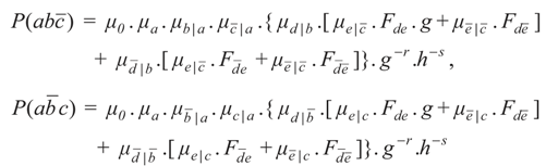
5. µ-Notation
The General Tribus Formula (Equation 8) contains a product of terms which represents a joint probability. This formula will now be expressed in a more compact form designed to facilitate further work, viz.:
where , and the index j ranges over the relevant constraints.
This notation was suggested by Garside [25]. The will be described as contributions from their respective constraints. At this point, the contributions from the set of linear constraints for a given probability group will be combined into a single combined contribution, to give a more economical representation. This is illustrated by the following example system which relates seven propositional variables, a..g.
5.1. Example 1
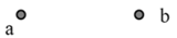
The moral graph for Figure 1 requires that vertices a and b, the parents of d, be joined (dashes), and also c and d, the parents of e, together with b and e the parents of f. If the network is to be triangulated, then b and c have to be joined (dots) as well.
5.1.1. Linear Constraints
For this network to be complete, values for the following set of probabilities must be made available (see Section 1):
This would imply eighteen contributions, but economy reduces this to seven combined contributions (underlined), one for each group of probabilities.
5.1.2. Independence Constraints
Method 2 requires both moral (the first two rows below) and triangulation independence constraints for a solution; a suitable set, see [17], is:
Economy reduces the contributions for the independence constraints to four.
Using µ-notation, a typical joint probability, , can now be expressed as:
where the suffixes locate the combined contributions rather than i and j.
Here, for example:
and:
5.2. Using Method 3 with µ-Notation
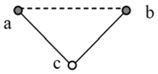
Early experiments with this method applied to a series of causal systems suggested that this algorithm, when given a full set of moral independencies, would generate the triangulation independencies required by Method 2. With this possibility in mind, the discussion will proceed by considering independence under Method 3 for a complete version of a system of six variables represented by a lozenge shaped network, Loz6. (nb. A lozenge will have at least five sides.)
Example 2: In Figure 2, given the moral independency for the sink vertex f, , analysis will be employed in an attempt to show that the non-moral independencies c cid d | b and b cid c | a, are implied.
The independence constraints and , may be expressed as:
and:
Treating and as pseudo-linears gives:
and:
The state probabilities in all differentiate to give , and those in give , with similar results for the second constraint.
According to the General Tribus Formula (Equation 8), and reverting to individual exponentials for the independency, to allow closer examination, the respective contributions for states in and are and . These may be written, in terms of a multiplier (g), as and , say. A similar provision will be made for the states of de, using h therefore, following work in Section 3 above, the update formulæ for the Lagrange multipliers of the independency are:
and:
5.2.1. Grg-Elimination
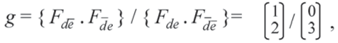
A method of deriving an independence constraint from a ratio due to G.R.Garside (outlined in a seminar) will now be described as it will be needed in ensuing sections:
Given:
this equals / after addition of the two numerators, and then the addition of the two denominators (this is a valid algebraic manipulation !)
i.e., /=/
or, after re-arrangement, /=/.
Adding numerators and denominators again:
which shows that y cid z | x, as required. This division and reduction technique will be referred to as grg-elimination and can be applied in reverse.
5.2.2. Analysis Phase 1: Determination of the Independence Multipliers
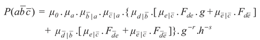
Assuming that a solution exists, the state probabilities will be calculated by the product of the combined contributions from the linear constraints, and the individual contributions from the moral independency in the form of powers of their multipliers. Using μ-notation, the joint probability now assumes the form:
also:
Adding these equations will eliminate f from the left-hand side, viz:
where:
Varying d and e will give:
and:
Now d cid e | c, which is given, implies that d cid e | abc. Therefore, the application of grg-elimination to the last four equations must result in complete cancellation, i.e.,
giving:
The right-hand side of this equation does not depend on c and so, by symmetry, h will return the same value, i.e., g = h, as confirmed by experiment.
NB. It can be seen that and have cancelled, leaving just ! This will be important in subsequent analysis.
5.2.3. Analysis Phase 2: Proof that c cid d | b
With the multipliers having been determined, the analysis can move on to testing one of the non-moral independencies. Starting with Equation 23:
and also:
Addition of these two equations leads to:
The following may be reached by a similar process:
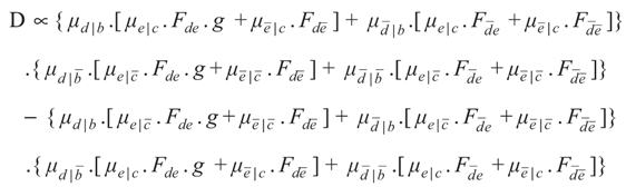
The condition required by grg-elimination is that:
or:
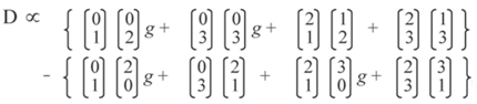
Representing the left-hand side of this identity by D, and noting that all the contribution terms cancel except for the four braces:
The result after multiplication is:
The first and fifth terms of this expression cancel, as do the fourth and eighth, giving:
But Equation 24 insists that g = {.} / {.}, therefore D 0 and the condition for grg-elimination is satisfied, giving the independency:
c cid d | ab
If this independency is compared with one given by d-Separation [9,18,21], a cid d | bc, then:
and:
division then gives:
Summation over , now gives the required independency, c cid d | b.
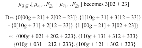
5.2.4. Tokenised Algebra
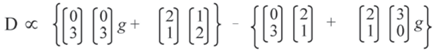
Consider Equation 25 again:
The author has devised a scheme whereby each term in the equation can be represented by its position within the set of possibilities for that term, for example:
As long as strict ordering is maintained it becomes possible to reduce the mass of algebraic manipulation. The current operation would start with:
D ∝ {00g + 21}.{12 + 33}_ {02 + 23}.{10g + 31}
Some simple arrays are needed to accommodate the result of the products:
 where the first array shows the product of and , and so on (it is to be noted that the elements are interchangeable in any such array).
The first and fifth terms cancel, as do the fourth and eighth to leave:
Considering the second array position:
 so:
so:

5.2.5. Analysis Phase 3: Proof that b cid c | a
To test this independency, Equation 23 (and similar equations) will be used as a starting point, but this time d and e will be removed:
and:
Addition applied to these four equations gives:
Likewise:
 and:
and:
The condition required by grg-elimination to establish the required independency is:
Let:
then, after cancelling, it follows that:
Applying tokens, where for example:
Multiplying out gives the difference of two sixteen term array sums. If they cancel out then the independency is established. The first term in the product is given by:
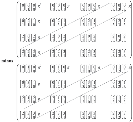
{000g }.{110g } to which is added the second term {000g}.{131}, etc.
All the terms cancel which are off the trailing diagonals in the two arrays. The remaining terms require the application of:
 to the third array in each element for cancellation. It follows that D ≡ 0 and so the independence constraint b cid c | a has been shown to be implied and, by a parallel process, b cid c | can be inferred.
The deduction can now be made that, given the explicit moral independencies, the triangulation independencies are induced in Loz6 under Method 3.
6. The Embedded Lozenge
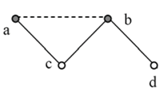
Method 3 required the linear constraints and just the moral independency to determine a solution for Loz6, but it remained to be discovered whether this property would persist with more general systems. An effort was made to provide a wider context, subject to non-violation of the lozenge (i.e., no lozenge vertices are directly linked across the figure). To this effect a generalised system Emb-LozN (see Figure 3 was considered, working along similar lines to those for Loz6.
6.1. A More General Example, Emb-LozN
The work in Section 4, was adapted to support a theoretical approach that used bottom-up analysis applied to Emb-LozN to prove that the moral independencies imply the conditional independence of variables 5 and 7. This required some rather complex and extended analysis, with combined contributions, that can be seen in [11] (or by correspondence with the author).
Having discovered the independency between 5 and 7, the relevant multipliers can be found by grg-elimination: they will share a common value. This new independency can now take the place of 3 cid 5 | 4,7 in an inductive scheme which ascends the graph discovering further independencies (the next one is between variables 7 and 9). Near the top of the graph, any odd edges of the lozenge and the apex itself will require some modification of earlier working, but it is not anticipated that this will create any major difficulty.
This analysis increases the scope of Method 3 considerably and opens up the possibility that the algorithm can be shown to apply over a wide range of complete systems.
To engineer results of complete generality the graph, or an algebraic equivalent, would have to be comprehensive. It might then be possible to deduce a result by either mathematical induction or by graph reduction.
The system in this section, Emb-Loz N (Figure 3, with vertices, is intended to mark a step towards such generality. An extended lozenge (double circles) has new network elements added so that that every vertex of the lozenge has the following two properties:
- (1)
- It is directly linked to both ancestors and descendants from among the new elements.
- (2)
- There are paths which bypass such a vertex.
Ideally the new elements should include vertices representing sets of variables but the work done was restricted to single variables because of the inherent algebraic complexity.
The graph displays an ancestral ordering, of single variables. The configuration at the top of the graph will depend on the number of sides to left and right.
The moral independency 3 cid 5 | 4,7 is given together with the set typified by:
2 cid 5 | 3,4 and 4 cid 7 | 5,6
6.2. Further Testing
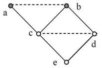
Another system, Random-Test8 (Figure 4), was subjected to examination to determine whether Methods 2, 3 and CNs gave coincident solutions.
Suitable Independence Sets for Figure 4:
For Method 2:
and:
For Method 3: The first three only.
a ind b, d cid f | e, g cid df | c
b cid d | ac, c cid f | de, e cid cd | b.
The augmented system was tested using the following linear constraints:
P(a) = 0.56, P(b) = 0.06,
P(d | ac) = 0.58, 0.53, 0.32, 0.49,
P(e | b) = 0.05, 0.49, P(f | e) = 0.88, 0.92, P(g | c) = 0.51, 0.61,
P(h | dfg) = 0.19, 0.40, 0.24, 0.45, 0.75, 0.58, 0.56, 0.70
The two algorithms and CNs produced identical solutions with entropy of:
4.526 672 923
Two lozenges embedded in Random-Test8 (see Figure 5 and Figure 6), sections of Figure 4, will now be used to illustrate the outcome of the analysis above:

Figure 5.
Loz1.
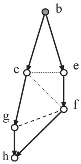
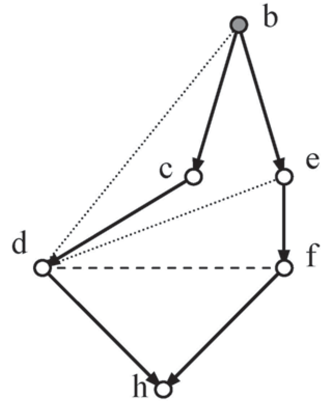
Figure 6.
Loz2.
Loz1 and Loz2, from Figure 4, exhibit their explicit moral independencies (dashes) and implied triangulation independencies (dots).
7. Discussion
The determination of the prior distribution of a causal network, using ME, by the three algorithms described, reveals their respective properties (NB. Some additional work was performed on incomplete networks).
7.1. Properties
Sequential ME
- Operates on complete networks,
- Requires d-seps1&2 to propagate probabilities,
- Suffers from rapid exponential complexity.
Development of Tribus
- Operates on complete and incomplete networks,
- Requires both triangulation and moral independencies,
- Can be used to validate CNs methodologies,
- Can be used to detect the stationary points for an incomplete
- network by varying the initial conditions,
- Potential for application beyond conventional networks.
Variation on Tribus
- Operates on complete networks only,
- Requires moral independencies alone,
- Potential for wider application,
- Further generalisation of proof needed.
7.2. Further Testing
A total of thirty systems were tested, including Loz6, Tree-Loz-Vee-Tri7, and Random-Test8. All the tests gave matching distributions under Methods 1,2,3 and CNs methodologies.
Method 1 relied on d-Separation alone and Method 3 required fewer explicit independencies than Method 2, as shown in Table 2.
Table 2.
Independence Averages.
8. Conclusions
Three methods for calculating the a priori probability distribution of a causal network, using ME, were discussed.
The first method used sequential determination of local probabilities, following a paper by Lukasiewicz, and this was illustrated with an example. Only the first two clauses of d-Separation were required in this process.
Method 2 started from the General Tribus Formula and aimed to find the over-all distribution directly. An algorithm was designed which required a set of explicit moral and triangulation independencies, in addition to the linear constraints. The technique for handling linear constraints served as a starting point for Method 3 where only the moral independencies and the linear constraints were required.
A novel representation of the General Tribus Formula, μ-Notation, was then used to represent the contributions from each constraint and was further developed by grouping similar terms. This divergence between Methods 2 and 3 was investigated by analysis applied to an elementary example. The investigation was then extended to a system of greater generality where Bottom-up analysis uncovered a method of finding implied independencies whilst climbing the graph. More work is needed to produce a result of complete generality.
A series of tests was undertaken to compare the independence requirements of the three methodologies. The results showed that Method 3 provides a more efficient method of solution than Method 2 over a significant range of complete causal network systems. Methods 2 and 3 have the potential to solve a wider range of problems than the CNs methodologies, therefore they constitute a useful augmentation of the technology available for solving problems in Expert Systems.
Acknowledgements
Suggestions and corrections were provided by R. S. Roberts (Durham).
References
- Griffeath, D.S. Computer solution of the discrete maximum entropy problem. Technometrics 1972, 14, 891–897. [Google Scholar] [CrossRef]
- Rhodes, P.C.; Garside, G.R. Use of maximum entropy method as a methodology for probabilistic reasoning. Knowl. Based Syst. 1995, 8, 249–258. [Google Scholar] [CrossRef]
- Neapolitan, R.E. Probabilistic Reasoning in Expert Systems: Theory and Algorithms; John Wiley & Sons: Hoboken, NJ, USA, 1990. [Google Scholar]
- Anderson, S.K.; Oleson, K.G.; Jenson, F.V.; Jenson, F. HUGIN-A Shell for Building Bayesian Belief Universes for Expert Systems. Proc. Int. Jt. Conf. Artif. Intell. 1989, 11, 1080–1085. [Google Scholar]
- Lauritzen, S.L.; Spiegelhalter, D.J. Local computations with probabilities on graphical structures and their applications to expert systems. J. Roy. Stat. Soc. B 1988, 50, 157–224. [Google Scholar]
- Jaynes, E.T. Where do we stand on maximum entropy? In The ME Formalism; The MIT Press: Cambridge, MA, USA, 1979. [Google Scholar]
- Paris, J.B.; Vencovská, A. A Note on the Inevitability of Maximum Entropy. Int. J. Approximate Reasoning 1990, 4, 183–223. [Google Scholar] [CrossRef]
- Shore, J.E.W.; Johnson, R.W. Axiomatic derivation of the principle of maximum entropy and the principle of minimum cross-entropy. IEEE Trans. Inform. Theory 1980, IT–26, 26–37. [Google Scholar] [CrossRef]
- Williamson, J.; Corfield, A.; Williamson, J. Foundations for bayesian networks. In Foundations of Bayesianism (Applied Logic Series); Kluwer: Dordrecht, The Netherlands, 2001; pp. 75–115. [Google Scholar]
- Williamson, J. Maximising entropy efficiently. Linköping Electron. Artic. Comput. Inform. Sci. 2002, 7, 1–32. [Google Scholar]
- Markham, M.J. Probabilistic independence and its impact on the use of maximum entropy in causal networks. Ph.D. Thesis, School of Informatics, Department of Computing, University of Bradford, Bradford, England, 2005. [Google Scholar]
- Paris, J.B. On filling-in missing information in causal networks. Int. J. Uncertainty Fuzziness Knowl. Based Syst. 2005, 13, 263–280. [Google Scholar] [CrossRef]
- De Campos, L.; Moral, S. Independence concepts for convex sets of probabilities. In Proceedings of the Eleventh Annual Conference on Uncertainty in Artificial Intelligence, Montreal, Canada, 18–20 August 1995; Morgan Kaufmann: San Francisco, CA, USA, 1995; pp. 108–115. [Google Scholar]
- Wally, P. Statistical Reasoning with Imprecise Probabilities; Chapman and Hall/CRC: Boca Raton, FL, USA, 1991; pp. 443–444. [Google Scholar]
- Lukasiewicz, T. Credal Networks under Maximum Entropy. In Proceedings of the 16th Conference on Uncertainty in Artificial Intelligence, Stanford, California, USA, July 2000; Morgan Kaufmann Publishers Inc.: San Francisco, CA, USA, 2000; pp. 63–70. [Google Scholar]
- Tribus, M. Rational Descriptions, Decisions and Designs; Pergamon Press: Elmsford, NY, USA, 1969; pp. 120–123. [Google Scholar]
- Markham, M.J. Independence in complete and incomplete causal networks under maximum entropy. Int. J. Uncertainty Fuzziness Knowl. Based Syst. 2008, 16, 699–713. [Google Scholar] [CrossRef]
- Geiger, D.; Verma, T.; Pearl, J. d-Separation: From theorems to algorithms. In Proceedings of the UAI’89 Fifth Annual Conference on Uncertainty in Artificial Intelligence; North-Holland Publishing Co.: Amsterdam, The Netherlands, 1990; pp. 139–148. [Google Scholar]
- Verma, T.S.; Pearl, J. Causal networks: Semantics and expressiveness. In Proceedings of the 4th AAAI Workshop on Uncertainty in AI; North-Holland Publishing Co.: Amsterdam, The Netherlands, 1988; pp. 352–359. [Google Scholar]
- Geiger, D.; Pearl, J. On the logic of causal models. In Proceedings of 4th AAAI Workshop on Uncertainty in AI; North-Holland Publishing Co.: Amsterdam, The Netherlands, 1988; pp. 136–147. [Google Scholar]
- Holmes, D.E. Independence relationships implied by D-separation in the bayesian model of a causal tree are preserved by the maximum entropy model. In Proceedings of the 19th International Worshop on Bayesian Interference and Maximum Entropy Methods, Boise, ID, USA, 2–6 August 1999; pp. 296–307.
- Grove, A.J.; Halpen, J.Y.; Koller, D. Random worlds and maximum entropy. J. Artif. Intell. Res. 1994, 2, 33–88. [Google Scholar]
- Hunter, D. Uncertain reasoning using maximum entropy inference. In Proceedings of the UAI-Uncertainty in Artificial Intelligence; Elsevier Science: New York, NY, USA, 1986; Volume 4, pp. 203–209. [Google Scholar]
- Shannon, C.E. A Mathematical Theory of Communication. Bell Syst. Tech. J. 1948, 27, 379–423. [Google Scholar] [CrossRef]
- Garside, G.R.; Rhodes, P.C. Computing marginal probabilities in causal multiway trees given incomplete information. Knowl. Based Syst. 1996, 9, 315–327. [Google Scholar] [CrossRef]


© 2011 by the author; licensee MDPI, Basel, Switzerland. This article is an open access article distributed under the terms and conditions of the Creative Commons Attribution license (http://creativecommons.org/licenses/by/3.0/).