Optimal Multi-Level Thresholding Based on Maximum Tsallis Entropy via an Artificial Bee Colony Approach

Abstract

This paper proposes a global multi-level thresholding method for image segmentation. As a criterion for this, the traditional method uses the Shannon entropy, originated from information theory, considering the gray level image histogram as a probability distribution, while we applied the Tsallis entropy as a general information theory entropy formalism. For the algorithm, we used the artificial bee colony approach since execution of an exhaustive algorithm would be too time-consuming. The experiments demonstrate that: 1) the Tsallis entropy is superior to traditional maximum entropy thresholding, maximum between class variance thresholding, and minimum cross entropy thresholding; 2) the artificial bee colony is more rapid than either genetic algorithm or particle swarm optimization. Therefore, our approach is effective and rapid.

2. Nonextensive Entropy

The entropy is basically a thermodynamic concept associated with the order of irreversible processes from a traditional point of view. Shannon redefined the entropy concept of Boltzmann/Gibbs as a measure of uncertainty regarding the information content of a system [23]. The Shannon entropy is defined from the probability distribution, where p_i denotes the probability of each state i. Therefore, the Shannon entropy can be described as:

(1)

where L denotes the total number of states. This formalism is restricted to the domain of validity of the Boltzmann-Gibbs-Shannon (BGS) statistics, which only describes Nature when the effective microscopic interactions and the microscopic memory are short ranged [24]. Suppose a physical system can be decomposed into two statistical independent subsystems A and B, the Shannon entropy has the extensive property (additivity):

(2)

However, for a certain class of physical systems which entail long-range interactions, long time memory, and fractal-type structures, it is necessary to use nonextensive entropy. Tsallis has proposed a generalization of BGS statistics, and its form can be depicted as:

(3)

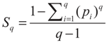where the real number q denotes an entropic index that characterizes the degree of nonextensivity. Above expression will meet the Shannon entropy in the limit q → 1. The Tsallis entropy is nonextensive in such a way that for a statistical dependent system. Its entropy is defined with the obey of pseudo additivity rule:

(4)

Three different entropies can be defined with regard to different values of q. For q < 1, the Tsallis entropy becomes a subextensive entropy where S_q(A + B) < S_q(A) + S_q(B); for q = 1, the Tsallis entropy reduces to an standard extensive entropy where S_q(A + B) = S_q(A) + S_q(B); for q > 1, the Tsallis entropy becomes a superextensive entropy where S_q(A + B) > S_q(A) + S_q(B).

The Tsallis entropy can be extended to the fields of image processing, because of the presence of the correlation between pixels of the same object in a given image. The correlations can be regarded as the long-range correlations that present pixels strongly correlated in luminance levels and space fulfilling.

3. Thresholding Model

Assume that an image can be represented by L gray levels. The probabilities of pixels at level i is denoted by p_i; so p_i ≥ 0 and p₁ + p₂ + … p_L = 1. If the image is divided into two classes, C_A and C_B by a threshold at level t, where class C_A consists of gray levels from 1 to t and C_B contains the rest gray levels from t + 1 to L, the cumulative probabilities can be defined as:

(5)

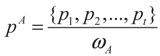
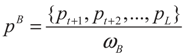
Therefore, the normalization of probabilities p^A and p^B can be defined as:

(6)

(7)

Now, the Tsallis entropy for each individual class is defined as:

(8)

(9)

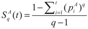
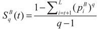
The Tsallis entropy S_q(t) of each individual class is dependent on the threshold t. The total Tsallis entropy of the image is written as follows [25]:

(10)

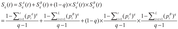
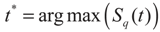
The task is to maximize the total Tsallis entropy between class C_A and C_B. When the value of S_q(t) is maximized, the corresponding gray-level t^* is regarded as the optimum threshold value:

(11)

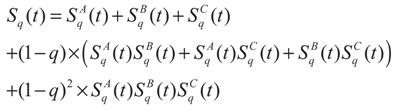
For bi-level thresholding, the best threshold can be obtained by a cheap computation effort, however, for multi-level thresholding (suppose the number of class is m), the problems will encounter following two challenges: 1) The optimization functions become more complicated. Considering a tri-level thresholding, the optimization function can be depicted as:

(12)

This causes little trouble since computers can calculate the function rapidly. 2) The parametric space is enlarged exponentially. The number of S_q(t) calculated is equal to:

(13)

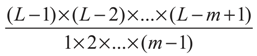
We choose m varying from 2 to 7 as examples and show the results in Table 1. It indicates the number of function calculated also increase from 255 to 3.6 × 10¹¹. Therefore, the exhaustive algorithm failed for multi-level thresholding, we will introduce the ABC method for fast computation in next section.

Table 1. Computation burden increases with the number of classes.

No of Classes m	2	3	4	5	6	7
No of Sq(t) calculated	255	32,385	2.73×106	1.72×108	8.64×109	3.60×1011

Table 1. Computation burden increases with the number of classes.

No of Classes m	2	3	4	5	6	7
No of Sq(t) calculated	255	32,385	2.73×106	1.72×108	8.64×109	3.60×1011

4. Artificial Bee Colony

4.1. Essential Components

In nature, each bee only performs a single task, whereas, through a variety of information communication ways between bees such as waggle dances and special odor, the entire bee colony can easily find food resources that produce relative high amounts of nectar, hence realize its self-organizing behavior [21]. In order to introduce the self-organization model of forage selection that lead to the emergence of collective intelligence of honey bee colony, we should define three essential components [26]:

• Food Resource: The value of a food source depends on different parameters, such as its proximity to the nest, richness of concentration of energy, and the ease of extracting this energy. For the simplicity, the profitability of a food source can be represented with a single quantity.
• Unemployed Foragers: If it is assumed that a bee has no knowledge about the food sources in the search field, it initializes its search as an unemployed forager looking for a food source to exploit. There are two types of unemployed forages: (I) Scouts: If the bee starts searching spontaneously without any knowledge, it will be a scout bee. The percentage of scout bees varies from 5% to 30% according to the information into the nest. The mean number of scouts averaged over conditions is about 10% in Nature [27]. (II) Onlookers: The onlookers wait in the nest and find a food source through the information shared by employed foragers. If the onlookers attend a waggle dance done by some other bee, the bees become recruits and start searching by using the knowledge from the waggle dance.
• Employed Foragers: Employed foragers are associated with a particular food source, which they are currently exploiting or are “employed” at. They carry with them information about this particular source, its distance and direction from the nest, and the profitability of the source. They share this information with a certain probability. After the employed foraging bee loads a portion of nectar from the food source, it returns to the hive and unloads the nectar to the food area in the hive. There are three possible options related to the residual amount of nectar for the foraging bee: (I) Unemployed Forager: If the nectar amount decreases to a low level or becomes exhausted, the foraging bee abandons the food source and become an unemployed bee. (II) Employed Forager 1: Otherwise, the foraging bee might dance and then recruit nest mates before returning to the same food source. (III) Employed Forager 2: Or it might continue to forage at the food source without recruiting other bees.

4.2. Principles and Procedures

At the initial stage, all the bees without any prior knowledge play the role of unemployed bees. There are two options for such a bee, viz. it can be either a scout or an onlooker. After finding the food source, the bee utilizes its own capability to memorize the information and immediately starts exploiting it. Hence, the unemployed bee becomes an employed forager. The foraging bee takes a load of nectar from the source and returns to the hive, unloading the nectar to a food store. When the profit of the food source is lower than the threshold, it abandons the food source and again becomes an unemployed bee. When the profit of the food source is higher than the threshold, it can continue its foraging, either recruiting more bees or by itself.

In this way, an artificial bee colony is introduced by mimicking the behavior of natural bees to construct a relative good solution of realistic optimization problems. The colony of artificial bees contains three groups of bees: employed bees, onlookers and scouts. The first half of the colony consists of the employed artificial bees and the second half includes the onlookers [21]. For every food source, there is only one employed bee, viz., the number of employed bees is equal to the number of food sources. The employed bee of an abandoned food source becomes a scout. The search carried out by the artificial bees can be summarized as follows [21]: (I) Employed bees determine a food source within the neighborhood of the food source in their memory. (II) Employed bees share their information with onlookers within the hive and then the onlookers select one of the food sources. (III) Onlookers select a food source within the neighborhood of the food sources chosen by themselves. (IV) An employed bee of which the source has been abandoned becomes a scout and starts to search a new food source randomly.

The detailed main steps of the algorithm are given below:

• Step 1. Initialize the population of solutions x_ij (here i denotes the ith solution, and j denotes the jth epoch, i = 1, …, SN, here SN denotes the number of solutions) with j = 0:

  

  (14)

  here LB & UB represents the lower and upper bounds, which can be infinity if not specified. Then, evaluate the population via the specified optimization function;
• Step 2. Repeat, and let j = j + 1;
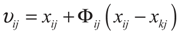
• Step 3. Produce new solutions (food source positions) υ_ij in the neighborhood of x_ij for the employed bees using the formula:

  

  (15)

  here x_kj is a randomly chosen solution in the neighborhood of x_ij to produce a mutant of solution x_ij, Φ is a random number in the range [−1, 1]. Evaluate the new solutions;
• Step 4. Apply the greedy selection process between the corresponding x_ij and υ_ij;
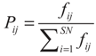
• Step 5. Calculate the probability values P_ij for the solutions x_ij by means of their fitness values using the equation:

  

  (16)

  here f denotes the fitness value;
• Step 6. Normalize P_ij values into [0, 1];
• Step 7. Produce the new solutions (new positions) υ_ij for the onlookers from the solutions x_ij using the same equation as in Step 3, selected depending on P_ij, and evaluate them;
• Step 8. Apply the greedy selection process for the onlookers between x_ij and υ_ij;
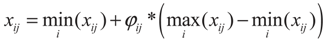
• Step 9. Determine the abandoned solution (source), if it exists, and replace it with a new randomly produced solution x_ij for the scout using the equation:

  

  (17)

  Here φ_ij is a random number in [0, 1].
• Step 10. Memorize the best food source position (solution) achieved so far;
• Step 11. Go to Step 2 until termination criteria is met.

5. Experiments

The experiments were carried out on a P4 IBM platform with a 3 GHz processor and 2 GB memory, running under the Windows XP operating system. The algorithm was developed via the signal processing toolbox, image processing toolbox, and global optimization toolbox of Matlab 2010b.

5.1. Effectiveness of Tsallis Entropy

We compared the maximum Tsallis entropy thresholding (MTT) to other criteria including maximum between class variance thresholding (MBCVT), maximum entropy thresholding (MET), and minimum cross entropy thresholding (MCET). Taking m = 2 as the example, suppose P^A and P^B denote the probability of class C_A and C_B, respectively, ω_A and ω_B denote the corresponding the cumulative probabilities, μ_A and μ_B denote the corresponding mean value, the formalism of objective function of different criteria are shown in Table 2. Here, we add a minus symbol to the objective function of MCET to transform the minimization to maximization.

Table 2. Objective function of different criteria (m = 2).

Criteria	Objective	Type
MET	S(A) + S(B)	Maximize
MBCVT	ωA × ωB × (μA − μB)2	Maximize
MCET	−μA × ωA × log(μA) − μB × ωB × log(μB)	Minimize
	μA × ωA × log(μA) + μB × ωB × log(μB)	Maximize
MTT	Sq(A) + Sq(B) + (1 − q) × Sq(A) × Sq(B)	Maximize

Table 2. Objective function of different criteria (m = 2).

Criteria	Objective	Type
MET	S(A) + S(B)	Maximize
MBCVT	ωA × ωB × (μA − μB)2	Maximize
MCET	−μA × ωA × log(μA) − μB × ωB × log(μB)	Minimize
	μA × ωA × log(μA) + μB × ωB × log(μB)	Maximize
MTT	Sq(A) + Sq(B) + (1 − q) × Sq(A) × Sq(B)	Maximize

We use some synthetic images to demonstrate the robustness of the MTT criteria. In the synthetic image, a square (gray value 192) is put on a background (gray value 64), and then Gaussian noises (variances = 0.01) was added to the whole image, so the histogram of the image is two Gaussian peaks. The size of the image is 256-by-256 size, and the size of the foreground square is 180-by-180, so that the heights of the two Gaussian peaks of foreground and background are nearly the same.

In addition, we reduce the length of the foreground square to change the height ratio of the two Gaussian peaks, and lower the gray level of the background to enlarge the distance of the two Gaussian peaks. q is determined as 4 for all cases of synthetic images.

The results are chosen and shown in Figure 1, Figure 2 and Figure 3. In Figure 1, the two Gaussian peaks are nearly the same. The MET, MBCVT, and MTT can find the optimal threshold, while MCET locates the threshold a bit left. In Figure 2, we shrink the size of the foreground object, so the peak of the background is much higher than the peak of the foreground object. The MET and the MTT perform well with threshold as 128 while MBCVT and MCET obtained the threshold nearly at the position of the higher Gaussian peak.

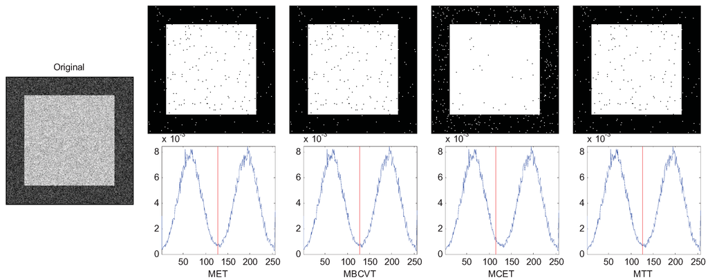
Figure 1. Segmentation of the synthetic image.

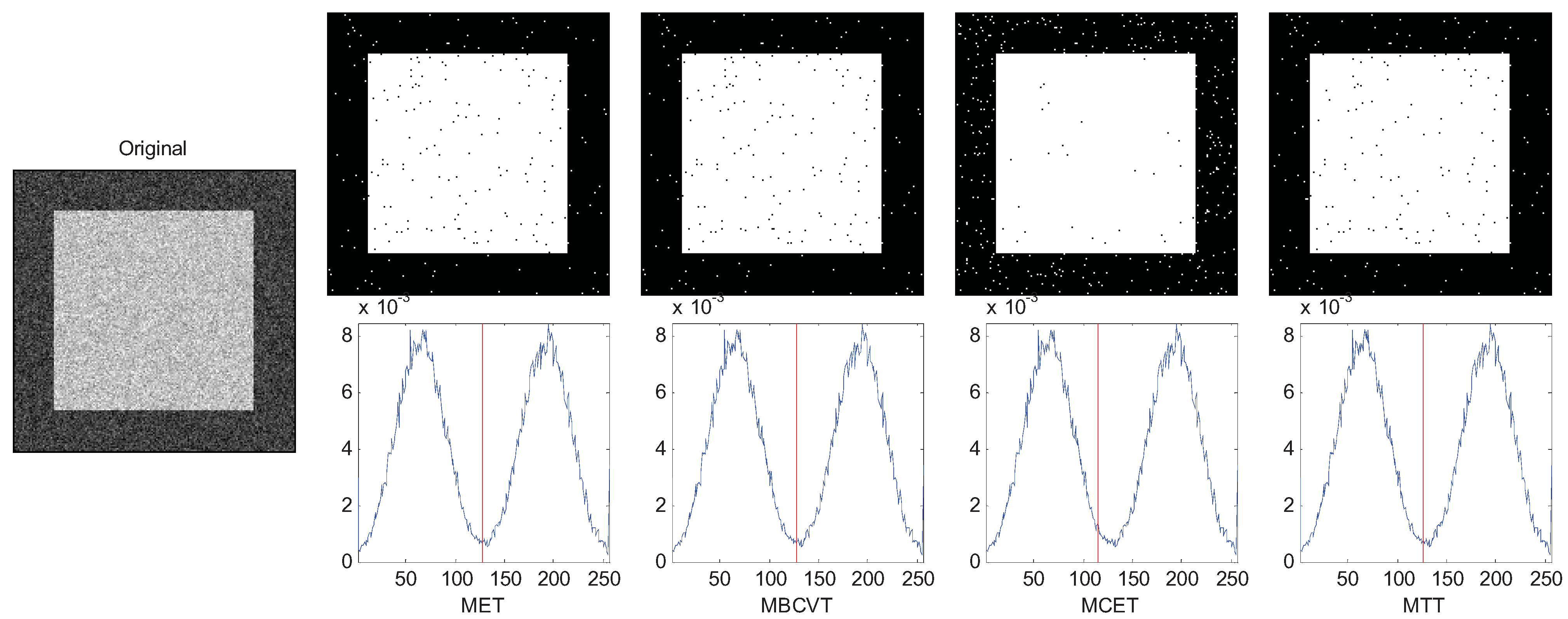
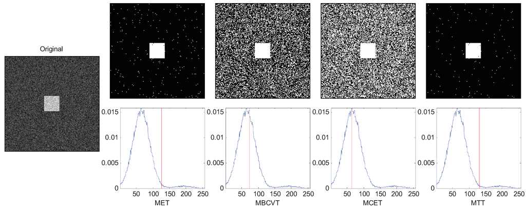
Figure 2. Segmentation of the synthetic image (foreground is smaller).

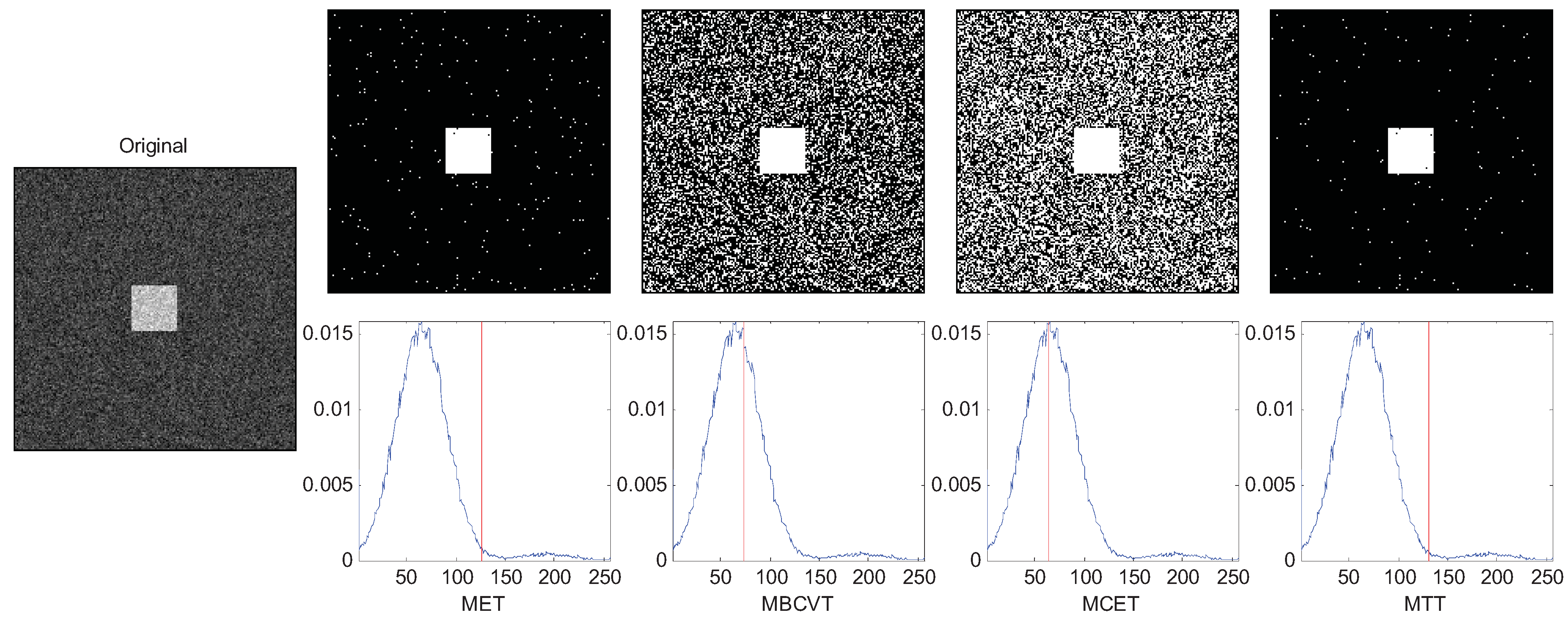
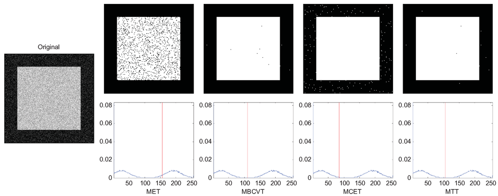
Figure 3. Segmentation of the synthetic image (background is darker).

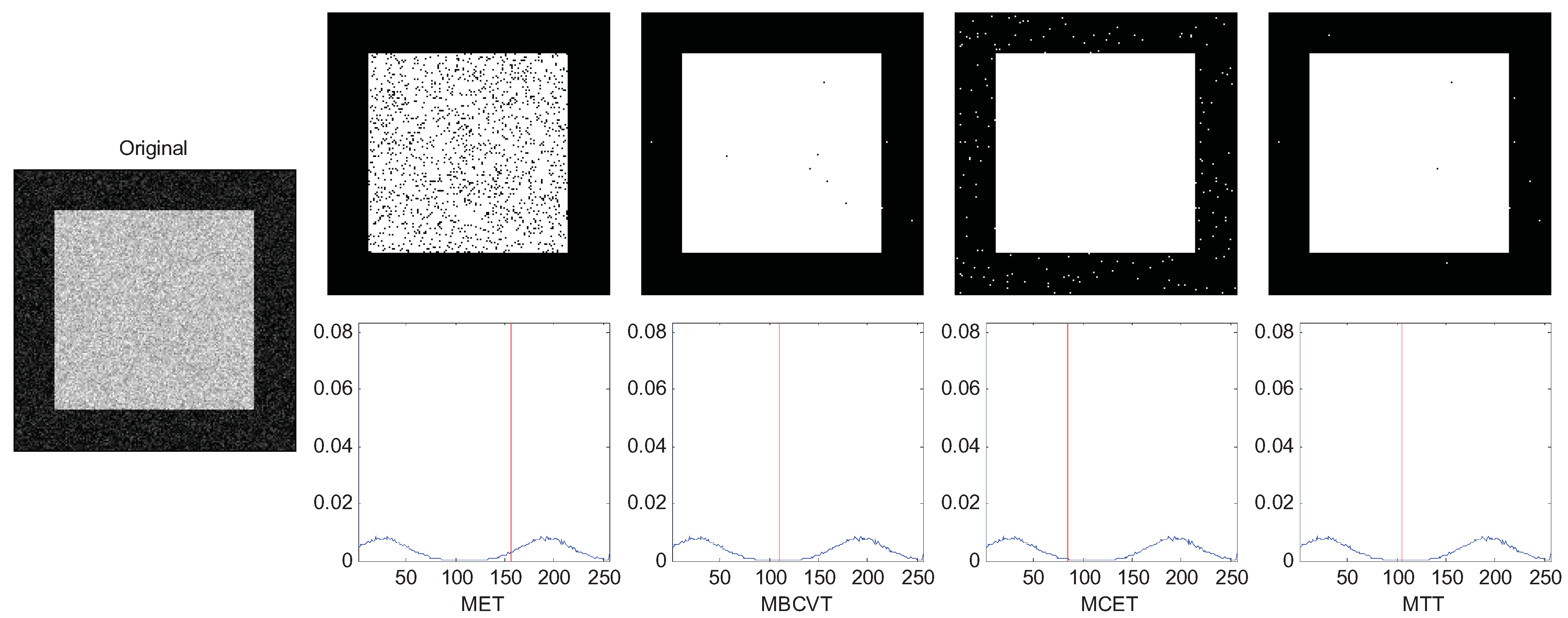
In Figure 3, we lower the gray level of the background to only 26 so that the distance between two peaks are further. In this case we observe that MBCVT and MTT obtain the right threshold just between the two peaks while MET finds a higher threshold and MCET finds a lower threshold. The results are listed in Table 3 which indicates that the MTT succeeds in all cases.

Table 3. Result of segmentation of synthetic image (√ denotes success).

Image	MET	MBCVT	MCET	MTT
Two equal Gaussian peaks	√	√		√
One peak is higher	√			√
Larger distance between two peaks		√		√

Table 3. Result of segmentation of synthetic image (√ denotes success).

Image	MET	MBCVT	MCET	MTT
Two equal Gaussian peaks	√	√		√
One peak is higher	√			√
Larger distance between two peaks		√		√

Afterwards, we compared the criteria with several real images, three of which are selected to demonstrate the effectiveness of MTT criterion. Figure 4 is an image of a flower with an inhomogeneous distribution of light around it. The Tsallis entropy criterion is very useful in such applications where we define a value for the parameter q to adjust the thresholding level to the correct point. In Figure 4 the image was segmented with q equal to 4. The thresholds of MET, MBCVT, MCET, and MTT are 126, 78, 42, and 14, respectively. It indicates that MTT obtains a cleaner segmentation without loss of any part of the flower.

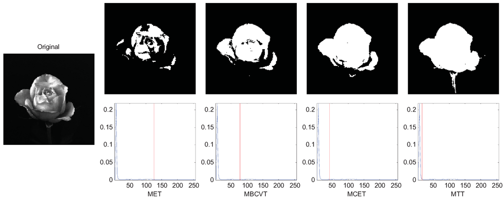
Figure 4. Segmentation of the rose image.

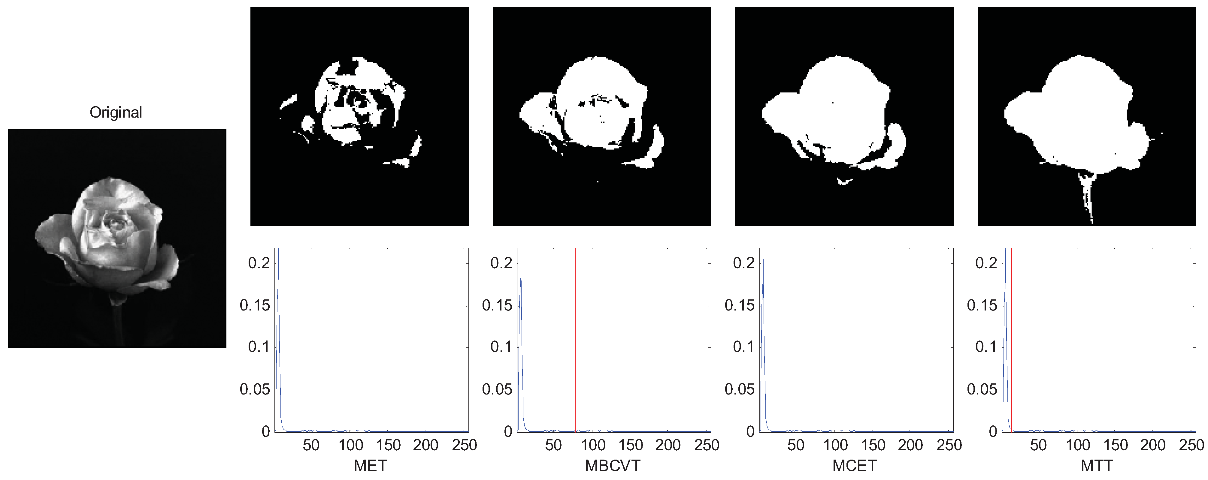
Figure 5 is an image of a tree in the right and leaves in the top-left corner. The q was set to 5. The thresholds of MET, MBCVT, MCET, and MTT are 114, 52, 35, and 63, respectively. Figure 5 shows that MTT extracts leaves in the top-left corner more completely than those by MET, MBCVT, and MCET. Therefore, the MTT outperforms again.

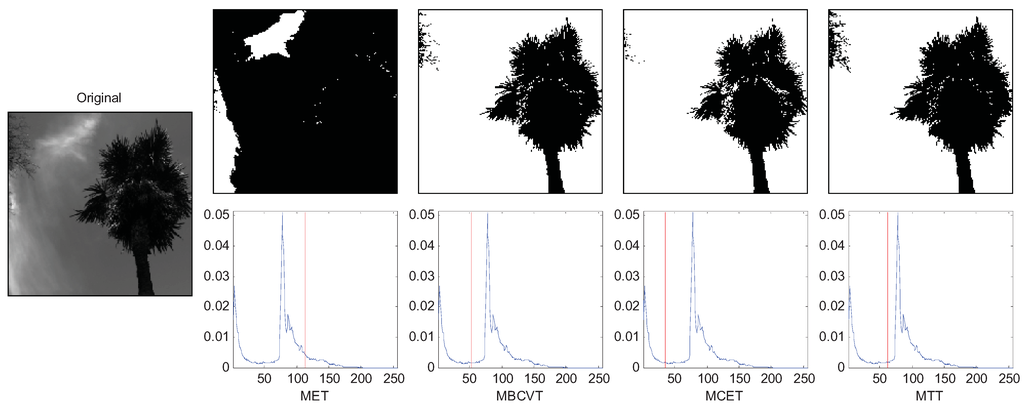
Figure 5. Segmentation of the tree image.

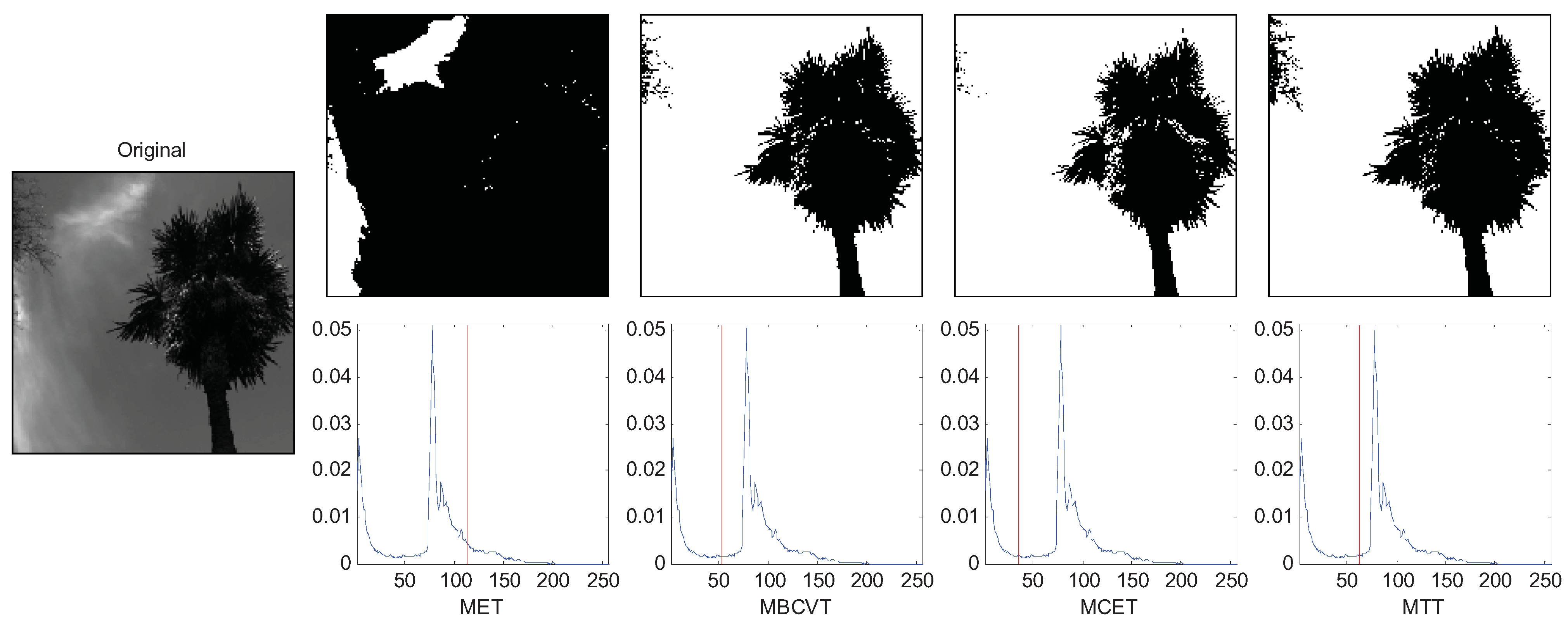
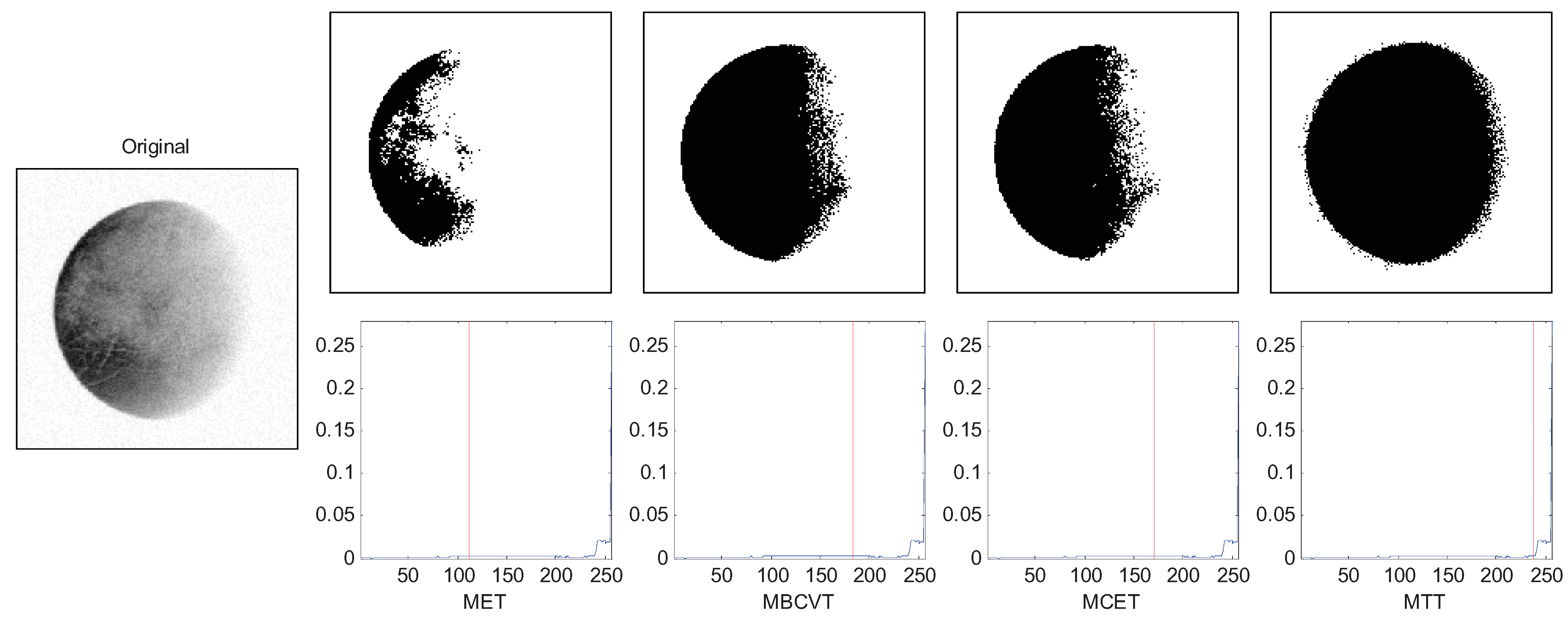
Figure 6 shows an image of Pluto. The q was set to 4. The thresholds of MET, MBCVT, MCET, and MTT are 111, 183, 170, and 238, respectively. It indicates that the MTT method obtains a fuller Pluto segmentation.

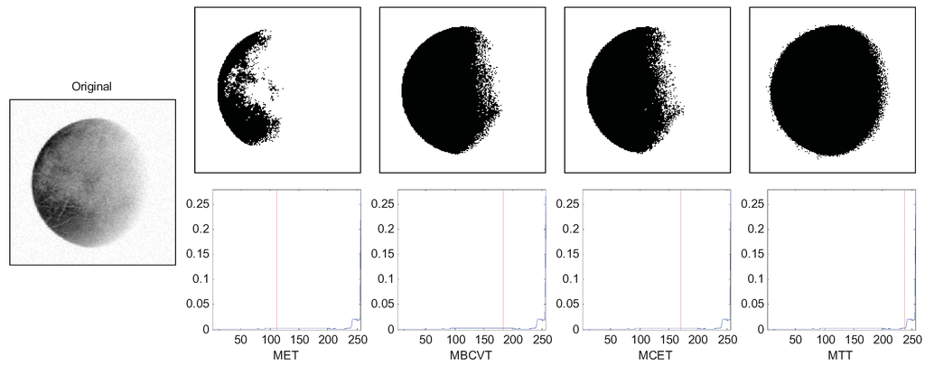
Figure 6. Segmentation of the Pluto image.

5.2. Rapidness of the ABC

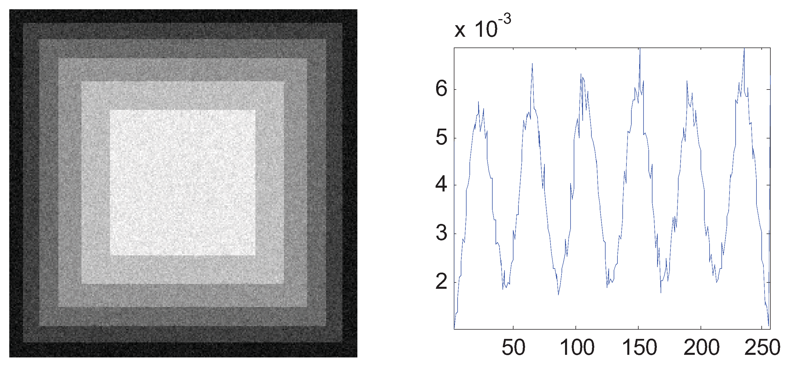
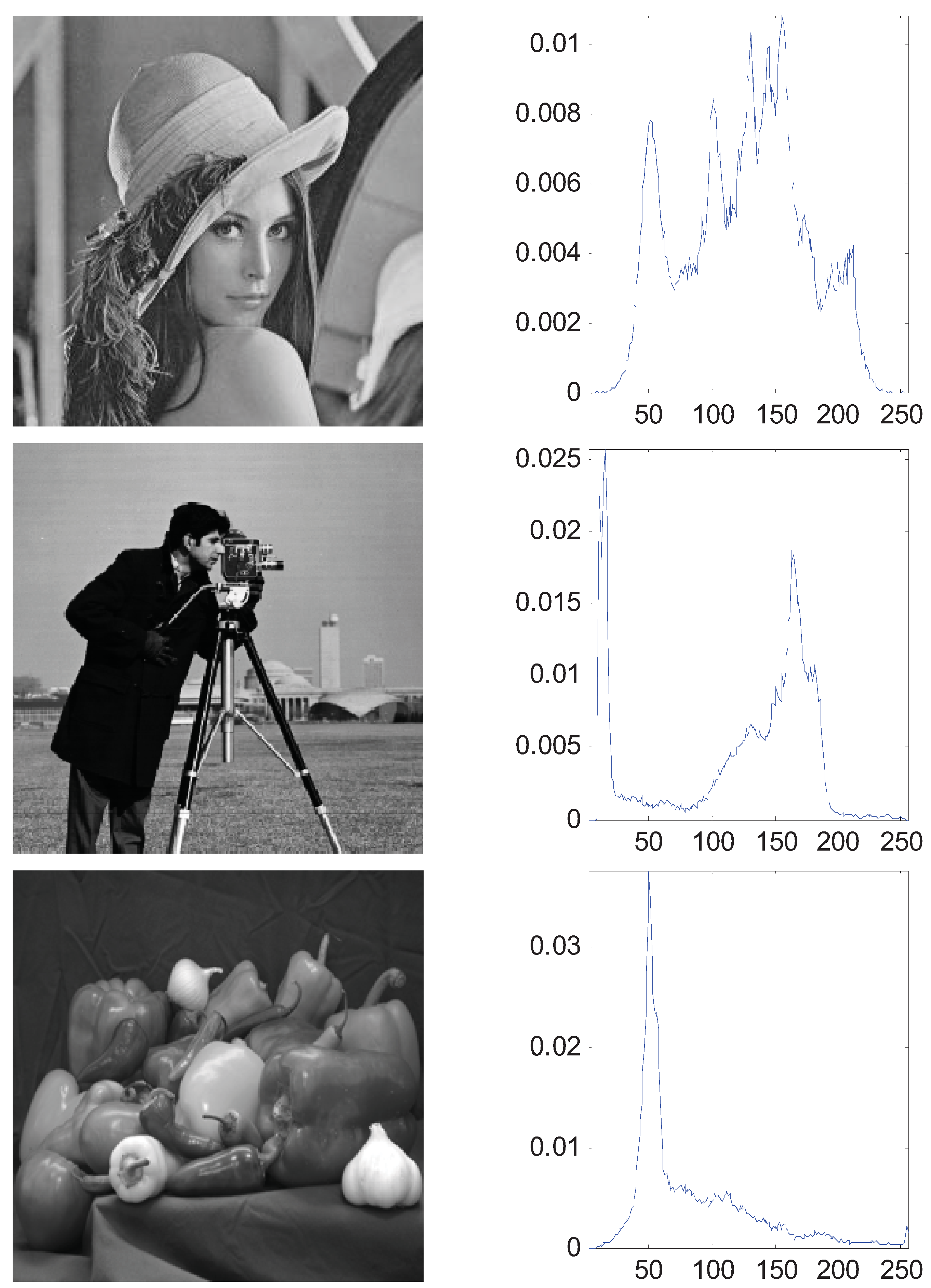
The aforementioned simulation experiments have proven the superiority of the MTT criterion. In this section, we generalize the bi-level thresholding to multi-level thresholding which needs the proposed ABC algorithm for fast computation. A synthetic image (A central square and five surrounding borders) and three real images of 256-by-256 pixels with corresponding histograms were used and shown in Figure 7. In order to evaluate and analyze the performance of ABC, we use the GA and PSO as the comparative algorithms. Each algorithm was run 30 times to eliminate the randomness.

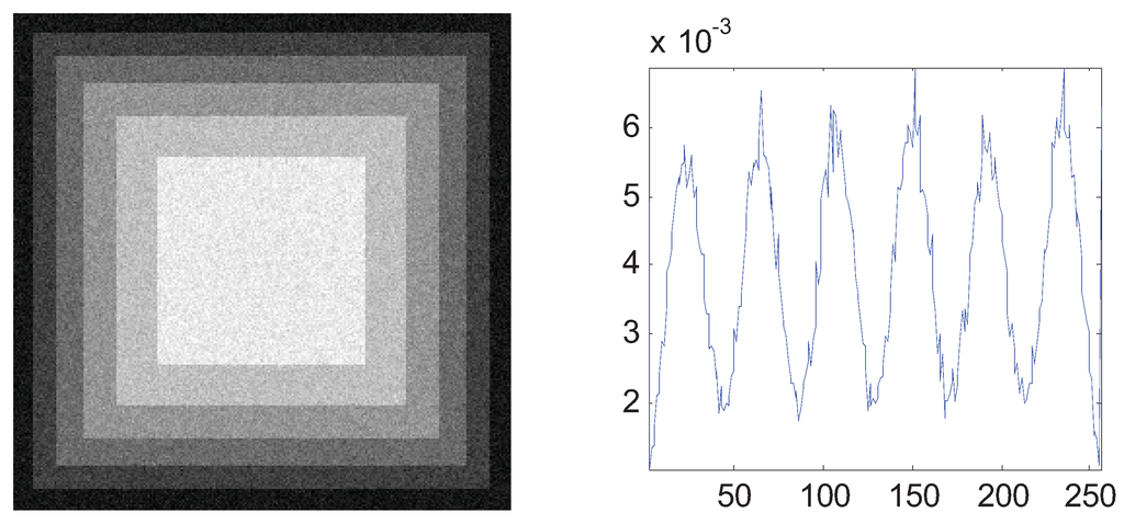
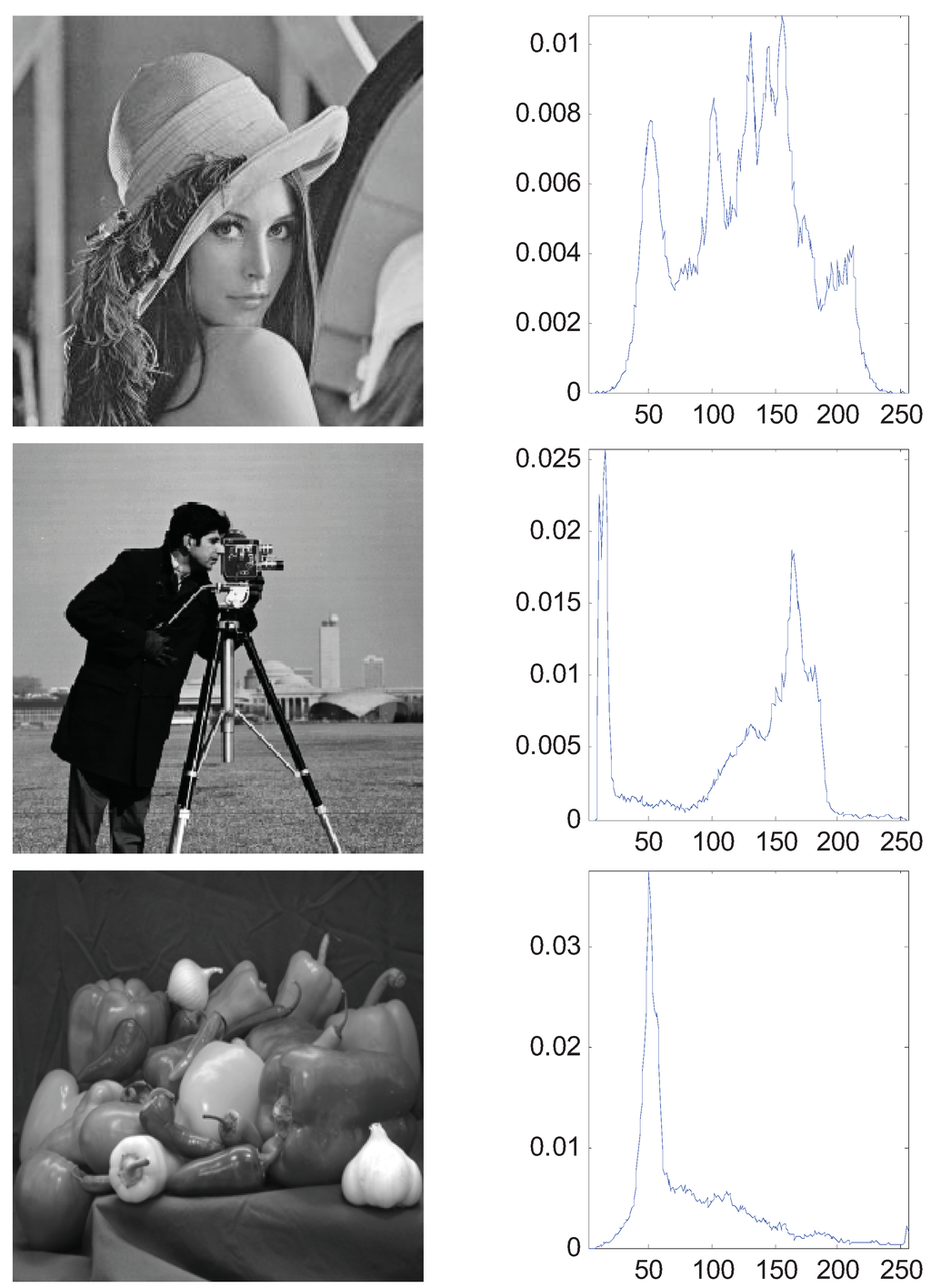
Figure 7. Four test images and the histograms: (a) synthetic (b) Lena; (c) cameraman; (d) peppers.

A typical run of the resulting segmentation for the four test images based on MTT are shown in Table 4, Table 5, Table 6 and Table 7, respectively, for classes m = 3 to 6 with segmented thresholds listed below. The selected thresholds by the ABC are nearly equivalent to the ones obtained by GA and PSO, which reveals that the segmentation results depend heavily on the criterion function selected.

Table 4. Multi-level segmentation for synthetic image.

m	GA	PSO	ABC
3
	89 172	85 171	85 170
4
	63 127 188	64 126 185	62 128 189
5
	52 99 157 205	49 100 155 205	50 101 155 204
6
	40 85 128 169 213	42 86 127 172 215	42 85 128 170 214

Table 4. Multi-level segmentation for synthetic image.

m	GA	PSO	ABC
3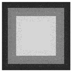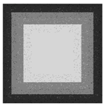
	89 172	85 171	85 170
4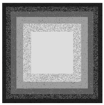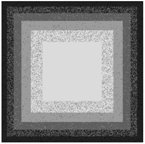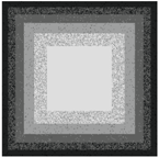
	63 127 188	64 126 185	62 128 189
5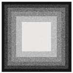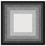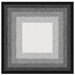
	52 99 157 205	49 100 155 205	50 101 155 204
6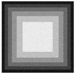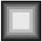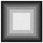
	40 85 128 169 213	42 86 127 172 215	42 85 128 170 214

Table 5. Multi-level segmentation for Lena image.

m	GA	PSO	ABC
3
	68 180	66 188	70 185
4
	73 112 192	67 113 187	71 113 188
5
	70 110 136 192	68 109 139 194	68 108 138 192
6
	68 111 136 168 187	69 112 134 169 188	69 110 135 169 189

Table 5. Multi-level segmentation for Lena image.

m	GA	PSO	ABC
3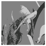
	68 180	66 188	70 185
4
	73 112 192	67 113 187	71 113 188
5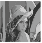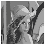
	70 110 136 192	68 109 139 194	68 108 138 192
6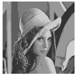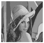
	68 111 136 168 187	69 112 134 169 188	69 110 135 169 189

Table 6. Multi-level segmentation for cameraman image.

m	GA	PSO	ABC
3
	102 199	95 199	99 195
4
	29 85 190	28 92 196	28 88 192
5
	27 93 144 195	31 88 141 197	29 90 141 195
6
	33 93 121 138 193	34 92 121 141 192	32 91 120 140 192

Table 6. Multi-level segmentation for cameraman image.

m	GA	PSO	ABC
3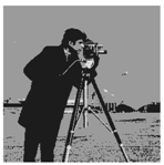
	102 199	95 199	99 195
4
	29 85 190	28 92 196	28 88 192
5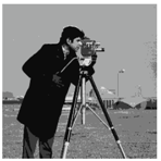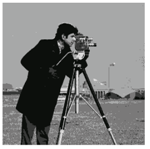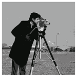
	27 93 144 195	31 88 141 197	29 90 141 195
6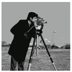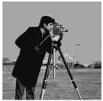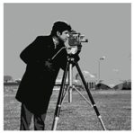
	33 93 121 138 193	34 92 121 141 192	32 91 120 140 192

Table 7. Multi-level segmentation for peppers image.

m	GA	PSO	ABC
3
	29 70	25 61	25 65
4
	23 64 111	24 69 106	26 66 108
5
	31 67 103 198	29 68 104 201	28 68 105 199
6
	30 70 106 147 204	31 70 104 146 201	30 70 104 148 203

Table 7. Multi-level segmentation for peppers image.

m	GA	PSO	ABC
3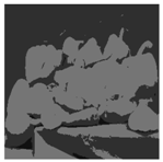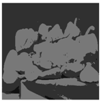
	29 70	25 61	25 65
4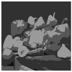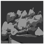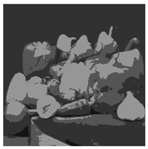
	23 64 111	24 69 106	26 66 108
5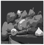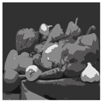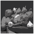
	31 67 103 198	29 68 104 201	28 68 105 199
6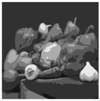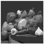
	30 70 106 147 204	31 70 104 146 201	30 70 104 148 203

Table 8 shows the average computation time of the three different methods for the four images with m = 3 to 6. As indicated in this table, with an increase in the class number m, the runtime tends to increase slowly due to the more complicated criterion function. For the Lena image, the computation algorithm of ABC increases from 1.6611 s to 1.7740 s when m increases from 3 to 6. Clearly, the efficiency of the intelligence optimization is far higher than traditional exhaustive method. Besides, the ABC costs the least time among all three algorithms.

Table 8. Average computation time (30 runs).

Image	m	GA	PSO	ABC
Synthetic	3	1.8849	1.8479	1.8210
	4	1.9487	1.8930	1.8316
	5	1.9780	1.9507	1.8709
	6	2.0453	2.0367	1.9807
Lena	3	1.9143	1.8931	1.6611
	4	1.9036	1.9115	1.6594
	5	2.0176	1.9500	1.7121
	6	2.1598	2.0577	1.7740
Cameraman	3	1.8755	1.7708	1.7083
	4	1.9168	1.8558	1.7003
	5	1.9686	1.8722	1.7975
	6	2.0175	1.9933	1.9191
Peppers	3	1.8890	1.8540	1.5321
	4	1.9636	1.8495	1.5527
	5	1.9985	1.9350	1.6924
	6	2.1395	2.0122	1.6484

Table 8. Average computation time (30 runs).

Image	m	GA	PSO	ABC
Synthetic	3	1.8849	1.8479	1.8210
	4	1.9487	1.8930	1.8316
	5	1.9780	1.9507	1.8709
	6	2.0453	2.0367	1.9807
Lena	3	1.9143	1.8931	1.6611
	4	1.9036	1.9115	1.6594
	5	2.0176	1.9500	1.7121
	6	2.1598	2.0577	1.7740
Cameraman	3	1.8755	1.7708	1.7083
	4	1.9168	1.8558	1.7003
	5	1.9686	1.8722	1.7975
	6	2.0175	1.9933	1.9191
Peppers	3	1.8890	1.8540	1.5321
	4	1.9636	1.8495	1.5527
	5	1.9985	1.9350	1.6924
	6	2.1395	2.0122	1.6484

5.3. Influence of the Parameter q

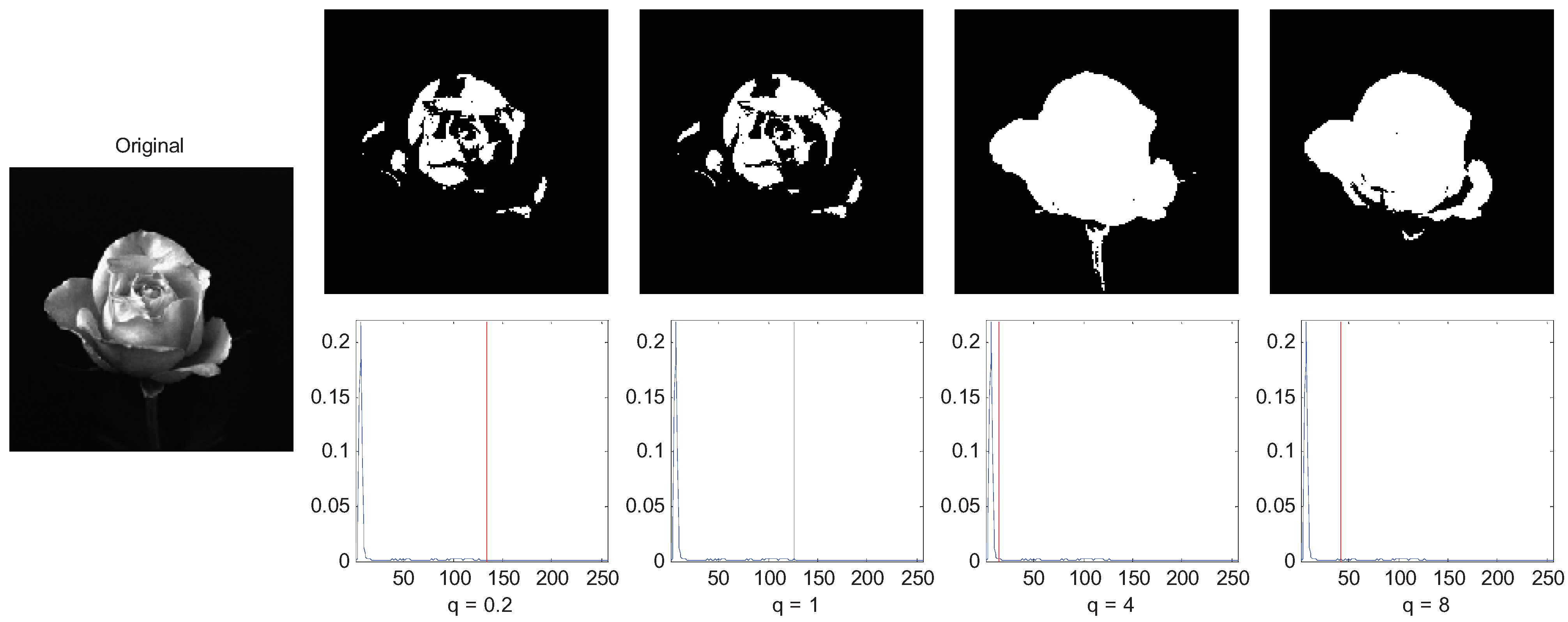
The final experiment is to demonstrate the influence of parameter q on the segmentation result. We use the rose image as the example and let q = 0.2, 0.5, 1, and 4. The segmentation results are shown in Figure 8. The rose image is a super-extensive system since the correlation of the pixels of the flower are long-range, so the MTT segmentation of q = 0.2 (sub-extensive) and q = 1(extensive) performed a non-satisfying segmentation result, and the MTT criterion of q = 4 segmented the rose image best. However, when q = 8, we do not get a good result since it corresponds to a too long-range correlation image.

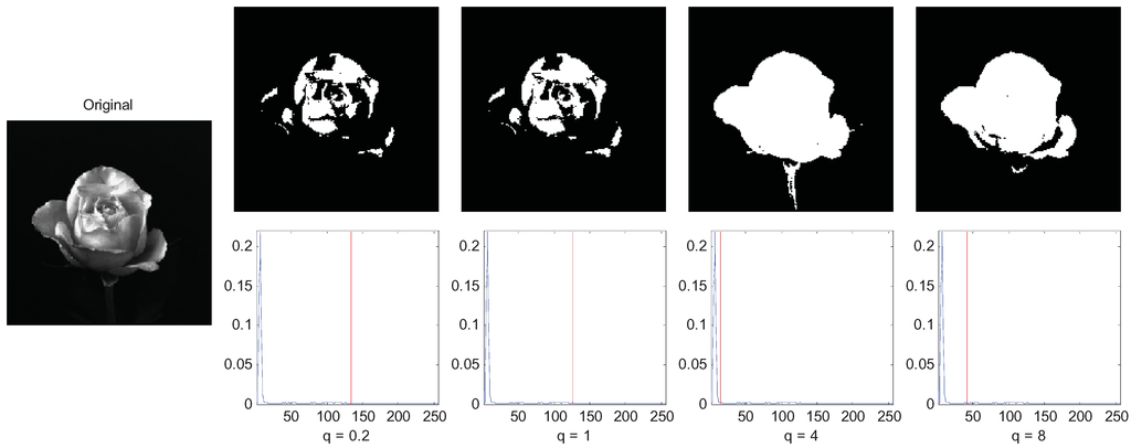
Figure 8. of long-range correlation image with variations of parameter q.

Another example is a texture image of which a large amount of foreground objects cluster together as shown in Figure 9, so the correlation between pixels of the same object is short range. In this case, the small q (q = 1) performs best.

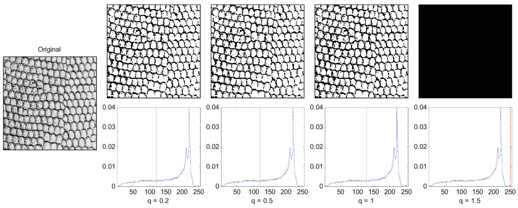
Figure 9. Segmentation of short-range correlation image with variations of parameter q.

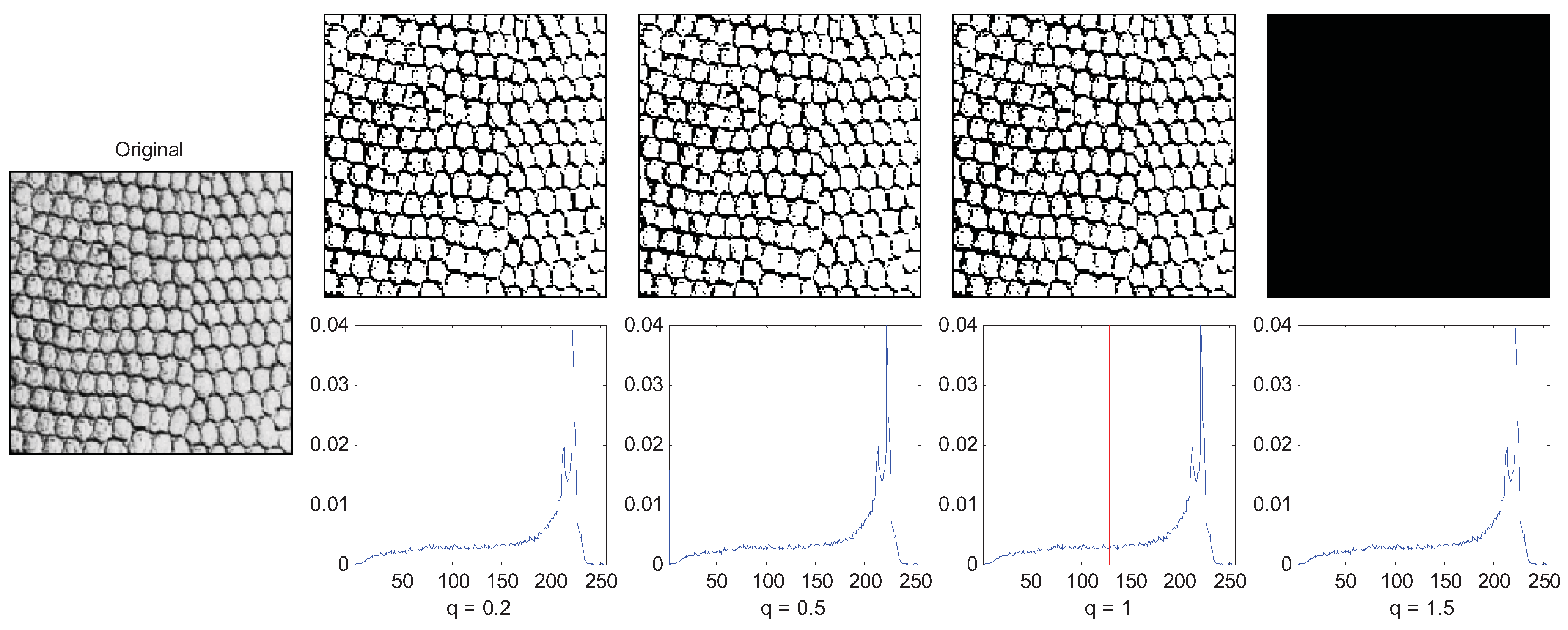
From the above two examples, we can see that the parameter q in an image is usually interpreted as a quantity characterizing the degree of nonextensivity. For image segmentation, the nonextensivity of the image system can be justified by the presence of correlations between pixels of the same object in the image. The correlations can be regarded as a long-range correlation in the case of the image that presents pixels strongly correlated in gray-levels and space fulfilling.

6. Conclusions

In this paper, we compared the maximum Tsallis entropy (MTT) with traditional criteria such as MBCVT, MET, and MCET. We found the segmentation by MTT can give better results than other criteria in many cases. When MTT is applied to multi-level thresholding, the ABC algorithm is introduced and it requires less time than GA and PSO. Therefore, the proposed method is both effective and rapid.

In the experimental section, we obtained all the values of q by a trial-and-error method. We found q = 4 performs good for most natural images, but for short-range correlation images, especially textured imaged, reducing the value of q will give better segmentation, and for some extremely-long correlation images, increasing the value of q is better. Nevertheless, there is no reliable evidence of a formal relationship between the parameter q and the image category.

The q parameter in the Tsallis entropy is used as an adjustable value, which plays an important role as a tuning parameter in the image segmentation. The future work will mainly focus on: 1) designing an automatic q-adjusting method and applying the Tsallis entropy to other industrial fields; 2) testing other nonextensive entropy including the Jensen-Tsallis divergence [16] and Renyi entropy [28].

References

- Lázaro, J.; Martín, J.L.; Arias, J.; Astarloa, A.; Cuadrado, C. Neuro semantic thresholding using OCR software for high precision OCR applications. Image Vision Comput. 2010, 28(4), 571–578. [Google Scholar] [CrossRef]
- Xue, Z.; Ming, D.; Song, W.; Wan, B.; Jin, S. Infrared gait recognition based on wavelet transform and support vector machine. Patt. Recog. 2010, 43(8), 2904–2910. [Google Scholar] [CrossRef]
- Anagnostopoulos, G.C. SVM-based target recognition from synthetic aperture radar images using target region outline descriptors. Nonlinear Anal.-Theor. Meth. App. 2009, 71(12), e2934–e2939. [Google Scholar] [CrossRef]
- Hsiao, Y.-T.; Chuang, C.-L.; Lu, Y.-L.; Jiang, J.-A. Robust multiple objects tracking using image segmentation and trajectory estimation scheme in video frames. Image Vision Comput. 2006, 24(10), 1123–1136. [Google Scholar] [CrossRef]
- Doelken, M.T.; Stefan, H.; Pauli, E.; Stadlbauer, A.; Struffert, T.; Engelhorn, T.; Richter, G.; Ganslandt, O.; Doerfler, A.; Hammen, T. 1H-MRS profile in MRI positive- versus MRI negative patients with temporal lobe epilepsy. Seizure 2008, 17(6), 490–497. [Google Scholar] [CrossRef] [PubMed]
- Wang, S.; Chung, F.-l.; Xiong, F. A novel image thresholding method based on Parzen window estimate. Patt. Recog. 2008, 41(1), 117–129. [Google Scholar] [CrossRef]
- Fan, S.-K.S.; Lin, Y. A multi-level thresholding approach using a hybrid optimal estimation algorithm. Patt. Recog. Lett. 2007, 28(5), 662–669. [Google Scholar] [CrossRef]
- Zahara, E.; Fan, S.-K.S.; Tsai, D.-M. Optimal multi-thresholding using a hybrid optimization approach. Patt. Recog. Lett. 2005, 26(8), 1082–1095. [Google Scholar] [CrossRef]
- Nakib, A.; Oulhadj, H.; Siarry, P. Non-supervised image segmentation based on multiobjective optimization. Patt. Recog. Lett. 2008, 29(2), 161–172. [Google Scholar] [CrossRef]
- Farrahi Moghaddam, R.; Cheriet, M. A multi-scale framework for adaptive binarization of degraded document images. Patt. Recog. 2010, 43(6), 2186–2198. [Google Scholar] [CrossRef]
- Chung, K.-L.; Tsai, C.-L. Fast incremental algorithm for speeding up the computation of binarization. Appl. Math. Comput. 2009, 212(2), 396–408. [Google Scholar] [CrossRef]
- Huang, D.-Y.; Wang, C.-H. Optimal multi-level thresholding using a two-stage Otsu optimization approach. Patt. Recog. Lett. 2009, 30(3), 275–284. [Google Scholar] [CrossRef]
- Wang, N.; Li, X.; Chen, X.-h. Fast three-dimensional Otsu thresholding with shuffled frog-leaping algorithm. Patt. Recog. Lett. 2010, 31(13), 1809–1815. [Google Scholar] [CrossRef]
- Horng, M.-H. A multilevel image thresholding using the honey bee mating optimization. Appl. Math. Comput. 2010, 215(9), 3302–3310. [Google Scholar] [CrossRef]
- Yin, P.-Y. Multilevel minimum cross entropy threshold selection based on particle swarm optimization. Appl. Math. Comput. 2007, 184(2), 503–513. [Google Scholar] [CrossRef]
- Hamza, A.B. Nonextensive information-theoretic measure for image edge detection. J. Electron. Imag. 2006, 15(1), 1–8. [Google Scholar]
- Parvan, A.S. Critique of multinomial coefficients method for evaluating Tsallis and Rényi entropies. Physica A 2010, 389(24), 5645–5649. [Google Scholar] [CrossRef]
- Nakib, A.; Oulhadj, H.; Siarry, P. Image thresholding based on Pareto multiobjective optimization. Eng. Appl. Artif. Intell. 2010, 23(3), 313–320. [Google Scholar] [CrossRef]
- Maitra, M.; Chatterjee, A. A hybrid cooperative-comprehensive learning based PSO algorithm for image segmentation using multilevel thresholding. Expert Syst. Appl. 2008, 34(2), 1341–1350. [Google Scholar]
- Karaboga, N.; Kalinli, A.; Karaboga, D. Designing digital IIR filters using ant colony optimisation algorithm. Eng. Appl. Artif. Intell. 2004, 17(3), 301–309. [Google Scholar]
- Karaboga, D.; Basturk, B. On the performance of artificial bee colony (ABC) algorithm. Appl. Soft Comput. 2008, 8(1), 687–697. [Google Scholar]
- Xu, C.; Duan, H.; Liu, F. Chaotic artificial bee colony approach to Uninhabited Combat Air Vehicle (UCAV) path planning. Aerosp. Sci. Technol. 2011, in press. [Google Scholar]
- Guida, A.; Nienow, A.W.; Barigou, M. Shannon entropy for local and global description of mixing by Lagrangian particle tracking. Chem. Eng. Sci. 2010, 65(10), 2865–2883. [Google Scholar]
- Campos, D. Real and spurious contributions for the Shannon, Rényi and Tsallis entropies. Physica A 2010, 389(18), 3761–3768. [Google Scholar]
- Portes de Albuquerque, M.; Esquef, I.A.; Gesualdi Mello, A.R. Image thresholding using Tsallis entropy. Patt. Recog. Lett. 2004, 25(9), 1059–1065. [Google Scholar]
- Kang, F.; Li, J.; Xu, Q. Structural inverse analysis by hybrid simplex artificial bee colony algorithms. Comput. Struct. 2009, 87(13–14), 861–870. [Google Scholar]
- Özbakir, L.; Baykasoglu, A.; Tapkan, P. Bees algorithm for generalized assignment problem. Appl. Math. Comput. 2010, 215(11), 3782–3795. [Google Scholar]
- Zarezadeh, S.; Asadi, M. Results on residual Rényi entropy of order statistics and record values. Inform. Sci. 2010, 180(21), 4195–4206. [Google Scholar]
© 2011 by the authors; licensee MDPI, Basel, Switzerland. This article is an open access article distributed under the terms and conditions of the Creative Commons Attribution license (http://creativecommons.org/licenses/by/3.0/).