2.1. Ideal Chain Model
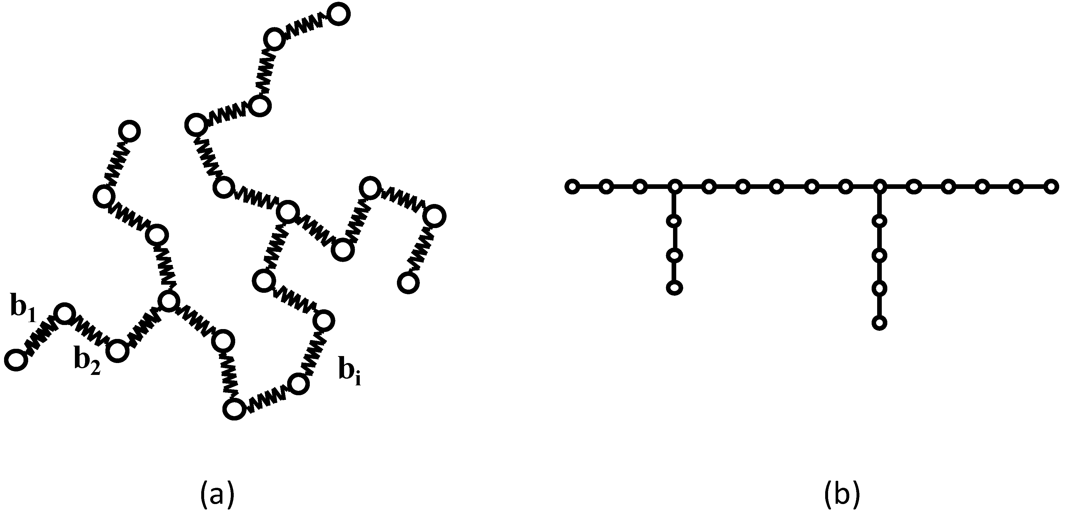
This article deals with the structural identification of tree-like chain molecules composed of the same repeat units without loops and rings like typical branched flexible homo-polymers. The dynamics and statics of isolated polymer molecules are usually examined in the equilibrium steady-state in order to identify their structural architecture. In the case of typical flexible vinyl polymers, a huge number of repeat units are connected by chemical single bonds. Although chemical bonds are fairly rigid with respect to stretching and bending of the valence angles between adjacent bonds, a single-polymer molecule has many internal degrees of rotational freedom about each actual bond in the molecule, resulting in the molecule adopting many different conformations, thereby necessitating the use of statistical mechanics. In the case of polyethylene, three types of micro-conformations, i.e., one trans and two gauche states, occur every C−C bond.
As described above, a polymer chain can take many different conformations in a dilute solution. This corresponds to the micro-Brownian motion and the chains are rapidly converted into other conformations. Each conformation exists for only a very short time so that the resulting conformations are temporal averages over all actual bonds. This results in the polymer chain being expressed by random-flight chains composed of statistical bonds (effective bonds) joining beads of unit mass where an appropriate number of actual bonds are replaced by a single effective bond. According to the central limit theorem in statistical physics [
4], the equilibrium distribution function of statistical bonds in random-flight chains is identical to the Gaussian distribution function. The distribution function
W(
bi) of the effective vector
bi between adjacent beads can be defined either as the time-averaged incidence of
bi within the specified range for a given molecule or as the average incidence for an ensemble of many identical units subject to identical conditions:
where <
b2> is the time-averaged square bond length, and the superscript T denotes the transpose of the vector and the matrix.
The probability distribution of the set of position vectors is given by the product of function W(bi). The change in entropy of the bond distribution is derived from the relation where kB is the Boltzmann constant. Since all conformations may have the same internal energy in the isothermal state, the change in the free energy is where T is the absolute temperature so that we have where and b be a 3 × (N − 1) matrix whose rows contain the dimensional component of the N−1 bond vectors between adjacent beads. Consequently, each effective bond can be considered to be a Hookean oscillator with a spring constant of . It should be noted that the spring constant is proportional to the temperature of the system. This means that the Hookean spring is associated with the dynamic potential based on the changes in conformational entropy.
Let
r be a 3 ×
N matrix whose rows contain the dimensional component of the
N position vectors of beads. The equilibrium state of this chain is then described by a distribution function proportional to
, where
V corresponds to the potential energy [
9], if we choose:
where Tr denotes the trace of matrix, and
Z is called the Zimm matrix in polymer dynamics [
5]. The
ijth element of matrix
Z is −1 if the
ith and
jth beads are directly connected; otherwise it is zero, and the diagonal elements are equal to the sum of its non-diagonal elements in a given row taken with the negative sign.
Z is the
N ×
N connectivity matrix which is known as the Laplacian matrix
L in graph theory.
2.2. Dynamics and Statistics of Gaussian Chains
If and only if the square root of
<b2> is identical with the effective bond length
b of the random-flight chain model, the random-flight statistics of a flexible polymer can be described by a Gaussian distribution function where the effective bonds can be represented as entropy springs called the segment [
6]. Rouse [
7] and Bueche [
8] demonstrated that the dynamics of a dilute solution of linear polymers can be characterized by considering a Gaussian chain suspended in a flowing viscous liquid. Subsequently, the extension of this model to any branched molecule was made by Ham [
9].
To consider linear dynamics in the ideal state for such bead-spring systems, we assume that each bead experiences an external force φ, then the equation of motion becomes:
This can be rewritten as follows using the bond vector b in place of the position vector r:
where
μ is the internal mass of each bead,
ζ is the friction constant of each bead and the matrix
R is (
N − 1) × (
N − 1) connectivity matrix which is called the Rouse matrix [
7]. Denoting by
the characteristic polynomial
of matrix
Z, where
I is the identity matrix of the same order as
Z, we can find the relation
[
10]. It should be noted here that these equations are applicable only to the unentangled polymers.
The eigenvalues of
Z contain one zero eigenvalue which represents the mode of chain transformation [
11]. A set of resonant eigen-frequencies of such system is obtained as follows by introducing the normalized coordinate transformation of Equation 3 or 4:
where
λp is a set of the eigenvalues of
R or non-zero eigenvalues of
Z and
ω0 is the primary frequency given by
. Each normal coordinate represents a mode of motion of the polymer chain. In addition, the relaxation time spectrum is written as:
where
τ0 =
ζ/κ. The relaxation times can be obtained by mechanical measurements in lower-frequency modes in which the inertial term in Equation 3 or 4 is neglected. In addition, the steady-state viscosity
η in a dilute solution can be obtained from the total sum of relaxation times and is given by [
12]:
where
ηs is the viscosity of pure solvent and
c is the concentration of beads per unit volume.
Forsman [
13] showed that the square radius of gyration of any random-flight (or Gaussian) chain can be given by
Consequently, the mean square of the radius of gyration can be expressed as:
It was found that not only the relaxation time and resonant frequency spectra but also the radius of gyration and steady-state viscosity of a single Gaussian chain with and without branching are entirely determined by a set of the eigenvalues of its Rouse matrix or the non-zero eigenvalues of its Zimm matrix. This means that the problem of identification of polymer chains is reduced to the problem of eigenvalues of the Rouse or Zimm matrix.
2.3. Graph-theoretical Approach
The mathematical representation of the graph theory is helpful in generalizing the statistics and dynamics of ideal chains to include in any type of branching [
3,
13,
14,
15,
16,
17,
18]. In graph theory, points (atoms or beads) are generally referred to as
vertices and lines (bonds or segments) are referred to as
edges, and the functionality of the beads is called the “
vertex degree”. Here we may consider only tree graphs in which every vertex has at least one and no loops or multiple edges are involved. The random-flight chain can be regarded as a molecular graph composed of
N − 1 statistical bonds (edges) of a length
b joining
N beads (vertices) of unit mass.
Figure 1 shows a Gaussian chain and its corresponding molecular graph.
Figure 1.
(a) An example of a branched Gaussian chain. (b) The corresponding molecular graph.
Figure 1.
(a) An example of a branched Gaussian chain. (b) The corresponding molecular graph.
In graph theory, the algebraic expressions using several matrices reflecting the connectivity in a graph
G [
19] are important devices for identifying the topological structure of graphs, and the algebraic properties of the characteristic polynomials have been extensively examined. For any graph
G, the adjacency matrix
A is the most fundamental matrix for the representation of graphs [
19] and it is defined as a square matrix in which
ijth element of matrix
A is 1 if the
ith and
jth beads are directly connected; otherwise it is zero.
The order of
A is identical with the total number of vertices in
G. The list of eigenvalues of a matrix calculated from the characteristic polynomial is called the spectrum of the matrix which includes a significant amount of quantitative information on the topological nature of the graphs. A secular determinant giving the Hückel molecular orbitals for the π electrons of an unsaturated hydrocarbon is reduced to the same form as the determinant of
A of its corresponding graph [
20,
21,
22]. In other words, the problem of the Hückel orbital energies can be completely reduced to the eigenvalue problem of
A. Thus, the spectrum of the matrix
A can be reduced to the energy levels of molecular orbitals.
A pair of graphs is said to be cospectral with respect to
A if they are non-isomorphic and their spectra are identical. A graph is said to be determined by the spectrum if there is no other non-isomorphic graph with the same spectrum. It has been identified that there are many pairs of nonisomorphic graphs with the same eigenvalue spectrum of
A. Theses pairs are considered to have the same energy levels under the Hückel approximation [
23,
24] but does not show always the identical photoelectron spectrum [
25].
The matrix
L defined as
, where
V is the diagonal matrix with the degree of vertex, is called the Laplacian matrix which has also widely been studied for topological connectivities of various graphs [
26]. The Laplace differential operator for a vibrating membrane can be transformed to the matrix
L by discretizing the Laplace equation [
27]. Immediately, we become aware that the Laplacian matrix is formally identical with the Zimm matrix; that is
. In addition, the signless Laplacian matrix
has the entries which are the absolute values of the entries of
L, and its polynomial equation is the same as that of
L. Consequently, the non-zero eigenvalues of
L+ or
L are identical with those of the Rouse matrix
R. Kirchhoff [
28] introduced a connectivity matrix
K for the calculation of currents in an electrical network and he found the relation
for tree-graph where
AL is the adjacency matrix for the line graph of the tree. The line graph of
G is formed by replacing the edges of
G by vertices in a manner such that the vertices in the line graph are connected whenever the corresponding edges in
G are adjacent. It is interesting to note that the elements of the matrix
K are the absolute values of the elements of
R and we have
[
16]. Consequently, we have the relation
using the relation
K =
AL + 2
I. The eigenvalues of
K of a tree graph or
R of a polymer chain can be obtained by adding 2 to the eigenvalues of
AL of its line graph.
The relations
and
have a very important meaning for polymer physics. The multiset of eigenvalues of
L or
AL is called the spectrum of
L or
AL. McKay [
29] found a mathematical technique for constructing a large number of pairs of Laplacian cospectral tree graphs or cospectral trees with cospectral line graphs. The probability that any tree graph is uniquely determined by its Laplacian spectrum goes to zero as the number of vertices approaches infinity [
30]. This means that almost all tree graphs cannot be uniquely determined by their Laplacian spectrum or line graph spectrum.
Theorem 1. There are many tree-like Gaussian chains with different branched structures showing the same resonance frequency or relaxation time spectrum.
Proof. The resonance frequency and relaxation time spectra as well as the radius of gyration of tree-like Gaussian chains were determined by a set of eigenvalues of the Rouse matrix or non-zero eigenvalues of the Zimm matrix. Since the Zimm matrix is identical to the Laplacian matrix, the resonance frequency and relaxation time spectra of the tree-like Gaussian chains can be determined by the Laplacian spectrum. There exist many Laplacian cospectral tree-graphs according to Mckay’s theorem [
29]. Consequently, there are many different tree-like Gaussian chains showing the same resonance frequency and relaxation time spectrum.
Theorem 1 has an important physical meaning. The proof shows that there are probably many pairs of different branched polymer chains showing the same relaxation time or resonance frequency spectra as well as the same radius of gyration. In other words, we may say that the determination of whether two flexible polymer structures are, or are not, identical is impossible by both dynamics and statics methods in the case that the polymer chains are represented by the intramolecular entropic forces and segmental friction.
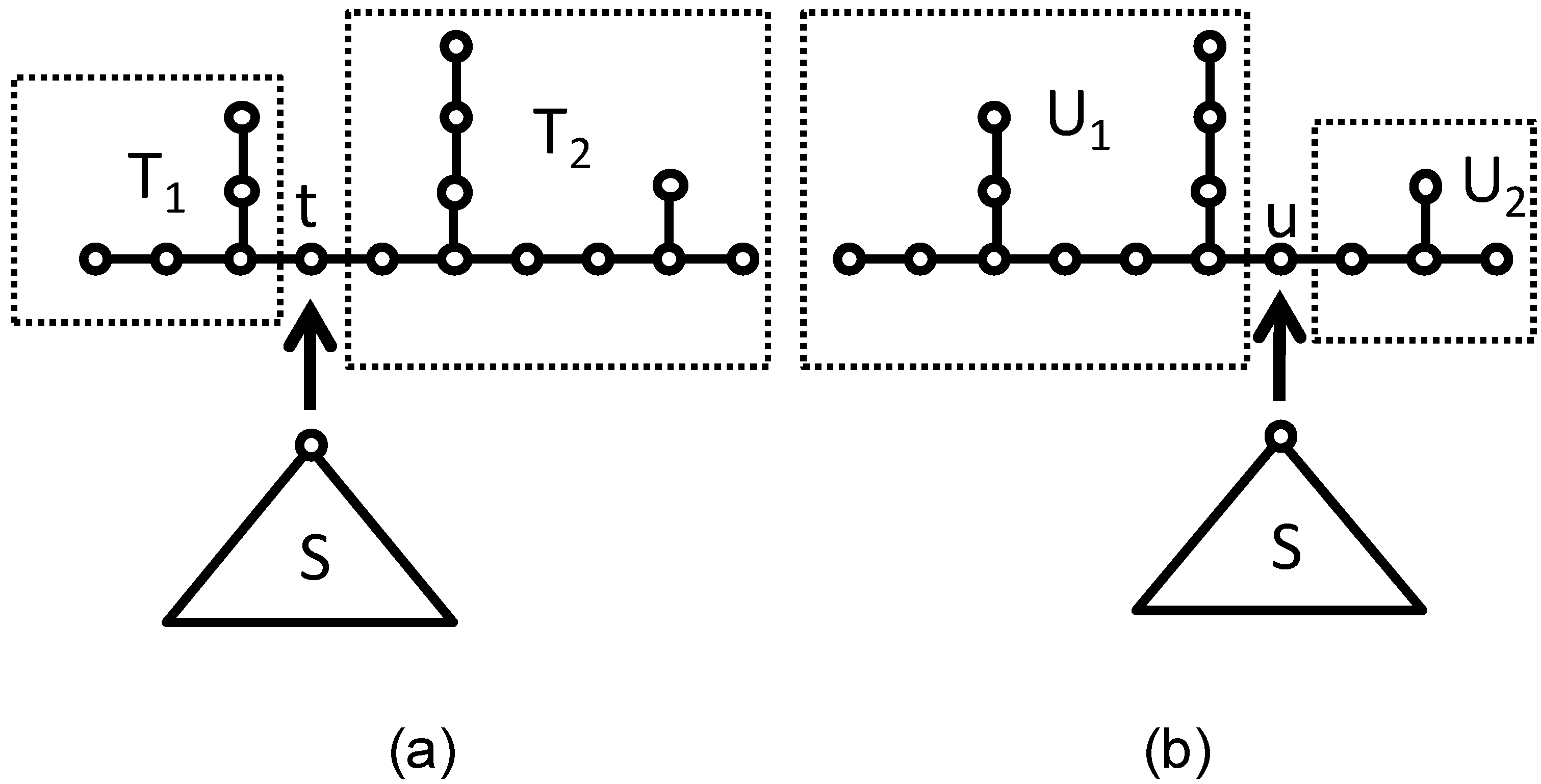
2.4. Example of the Laplacian Cospectral Trees
Here, we generalize McKay’s approach for constructing a pair of Laplacian cospectral trees. Let T or U be a tree divided in two subgraphs T
1 and T
2 or U
1 and U
2 by a root
t or
u (t ≠ u) with two degrees as shown in
Figure 2. Here T = U and these subgraphs are different from each other. The coalescence S·T of S and T is the tree formed by identifying the roots of S and T. Subsequently, S·T ≠ S·U. The forest T
1, T
2 formed by removing the root and its edges from T is denoted T* =T
1+T
2 and the incomplete tree formed by removing only the root of T is denoted T−
t where the degree of vertices connected to the root is unchanged by removing the root. The
V(T−
t) is defined to be the diagonal matrix of the degree of the vertex, except the root in T (not T*) as defined by McKay [
29].
Figure 2.
Images of a tree graph T composed of subgraphs T1 and T2 connected by root t and its T* and T−t graph.
Figure 2.
Images of a tree graph T composed of subgraphs T1 and T2 connected by root t and its T* and T−t graph.
Let S be any rooted tree with two or more vertices. The necessary and sufficient condition that S·T and S·U are cospectral with respect to Laplacian matrix: Φ(
L(S·T)) = Φ(
L(S·U)) is Φ(
A(T*) +
V(T −
t)) = Φ(
A(U*) +
V(U −
u)). The mathematical details are skipped here. McKay [
29] found an example for Laplacian cospectral graphs as shown in
Figure 3.
Figure 3.
(a) T1 graph and T2 graph; (b) U1 graph and U2 graph. Images of the coalescence process of S and T.
Figure 3.
(a) T1 graph and T2 graph; (b) U1 graph and U2 graph. Images of the coalescence process of S and T.
