Modeling the Underlying Drivers of Natural Vegetation Occurrence in West Africa with Binary Logistic Regression Method

Abstract

The occurrence of natural vegetation at a given time is determined by interplay of multiple drivers. The effects of several drivers, e.g., geomorphology, topography, climate variability, accessibility, demographic indicators, and changes in human activities on the occurrence of natural vegetation in the severe drought periods and, prior to the year 2000, have been analyzed in West Africa. A binary logistic regression (BLR) model was developed to better understand whether the variability in these drivers over the past years was statistically significant in explaining the occurrence of natural vegetation in the year 2000. Our results showed that multiple drivers explained the occurrence of natural vegetation in West Africa at p < 0.05. The dominant drivers, however, were site-specific. Overall, human influence indicators were the dominant drivers in explaining the occurrence of natural vegetation in the selected hotspots. Human appropriation of net primary productivity (HANPP), which is an indicator of human socio-economic activities, explained the decreased likelihood of natural vegetation occurrence at all the study sites. However, the impacts of the remaining significant drivers on natural vegetation were either positive (increased the probability of occurrence) or negative (decreased the probability of occurrence), depending on the unique environmental and socio-economic conditions of the areas under consideration. The study highlights the significant role human activities play in altering the normal functioning of the ecosystem by means of a statistical model. The research contributes to a better understanding of the relationships and the interactions between multiple drivers and the response of natural vegetation in West Africa. The results are likely to be useful for planning climate change adaptation and sustainable development programs in West Africa.

Highlights

• Underlying drivers of natural vegetation were identified by Binary Logistic Regression.
• Multiple underlying drivers were significant at p < 0.05 with varying impacts.
• Human activities indicators were the dominant underlying drivers.
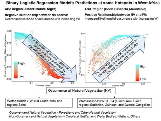
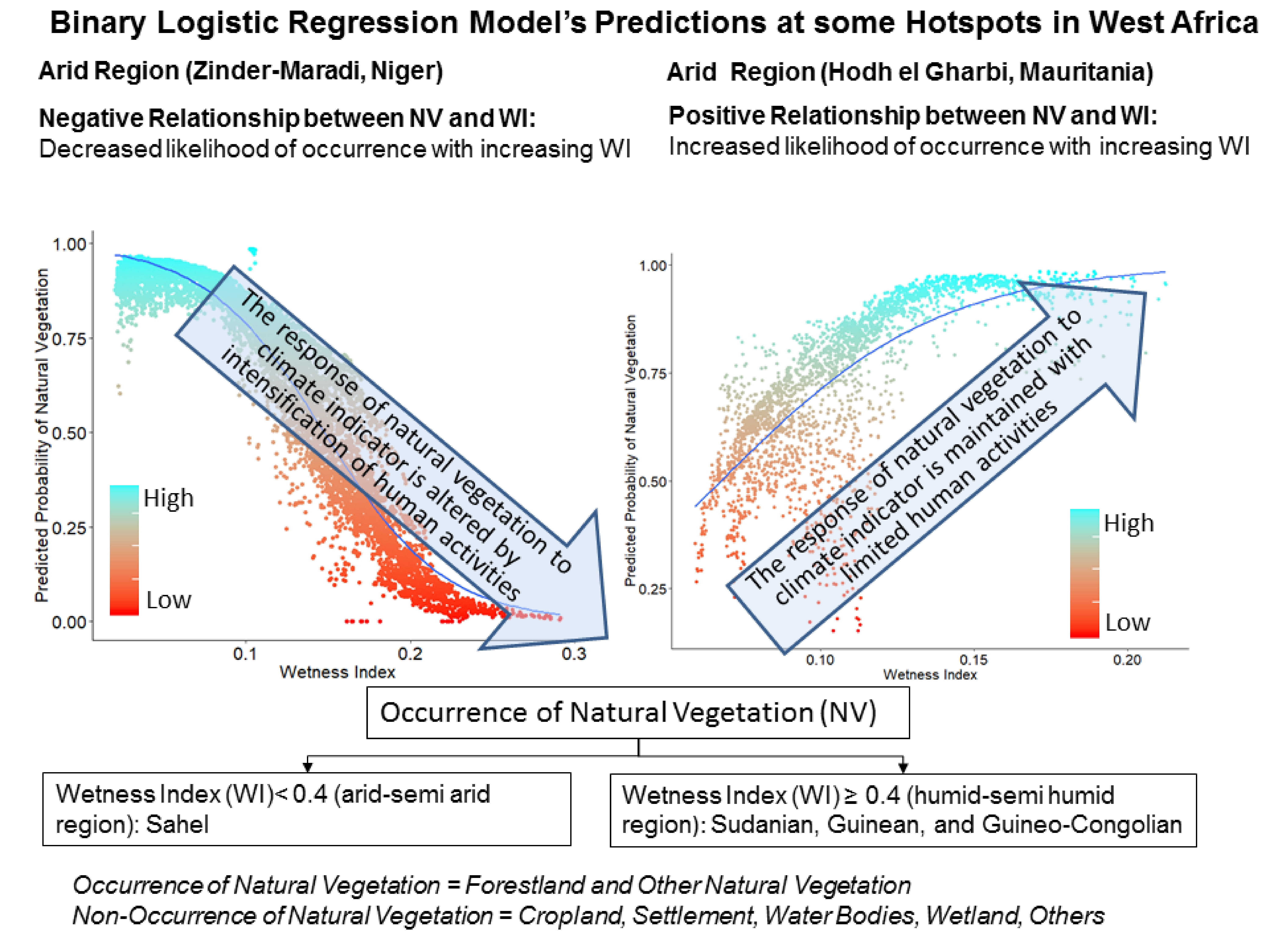
• The response of natural vegetation to climate was altered by intensification of human activities.

1. Introduction

Over the years, changes in the anthroposphere have drastically altered the normal functioning of the ecosystem, leading to widespread environmental deterioration, serious famine, and food security risks with a subsequent impact on the sustainable development and human well-being in many countries. According to Turner et al. [1] and Foley et al. [2], intensive anthropic (human) activities and the rapid changes in the Land Use Land Cover (LULC) system at the local, regional, and global scales may intensify changes in the land surface climate and exacerbate the vulnerability of the ecosystem to changes. Ecosystem changes, in some cases, are normal phenomena and a natural way for the system to regulate itself. The problem is that the pace and the magnitude at which the system is changing have been alarming in recent years due to over-exploitation by humans in light of population growth, abrupt changes in climate and intrinsic natural conditions (terrain slope, elevation, and soil type), improved accessibility to natural vegetation areas, and other multiple drivers [1,3]. According to Steffen et al. [4] and Ehlers and Krafft [5], in the past, human-induced LULC changes and, in particular, natural vegetation changes were restricted to a few areas and insignificant drivers of the ecosystem dynamics. In contrast, the current human impact on the ecosystem is pervasive and can be observed at a different spatial aggregation. The 1970s and 1980s drought and environmental disturbances in Africa [6] is a typical example of how the synergetic effect of multiple factors may lead to extreme environmental degradation, deforestation, biodiversity loss, food security risks, global warming, and so forth [7,8,9,10]. The consequences of it manifested through the LULC change of the continent, i.e., encroachment of natural vegetation by human-induced LULC types, e.g., cropland and settlements [11,12,13].

LULC change is, therefore, recognized as a major indicator of the impact of climate, anthropic activities, and other drivers on the ecosystem [14]. Lambin et al. [3] highlighted that the LULC change is a complex process driven by a combination of proximate and underlying drivers [15]. Human activities such as farming, illegal logging of timber, firewood extraction, and settlement expansions have a direct impact on the LULC system and may be categorized as proximate drivers [15]. According to Lambin et al. [3], proximate drivers are often under the direct control of the local people. On the other hand, the underlying drivers may be beyond the control of the indigenous people. In many cases, they are intrinsic natural characteristics, i.e., topography, climate, soil type, or accessibility to and from natural areas, socio-economic, e.g., poverty, agricultural, and development policies as well as demographic factors, e.g., human population growth with indirect impacts on the LULC system at the local level [3,14]. The previously mentioned multiple underlying causes of the LULC change have been considered by different theories to explain the underlying drivers of LULC change in the past. According to Chomitz and Gray [16], the drivers of LULC change may be explained by Boserupinan (1965) and Malthusian’s (1826) theories, which relate the LULC change to population growth, the von Thunen’s (1966) perspective, which relates the LULC change mainly to location-specific characteristics, such as cost of access to market, and the Ricardian (1817) theory, which relates the LULC change to intrinsic land quality (e.g., soil quality, slope, and elevation). Turner et al. [1] pointed out that these drivers are location-specific and context-specific.

In the context of Africa, especially the Sahel region, the school of thought is that climate variability (e.g., variation in wetness index) is the major underlying driver of natural vegetation’s change [17,18,19,20]. On the contrary, Lambin et al. [14] were of the view that climate variability alone is not sufficient to explain the natural vegetation change in Africa. Some other studies relate changes in natural vegetation to either population growth or improved accessibility, poverty, the land tenure system, and so forth [21,22,23,24]. Boschetti et al. [25], Brandt et al. [26], Rishmawi and Prince [27], and Leroux et al. [28] highlighted that interplay of multiple factors drive a natural vegetation change in Africa. At the sub-continental and continental scales of Africa, previous driving factors analysis focused on historical LULC change detection [11,12,13]. These studies [11,12,13] revealed LULC transitions at the expense of natural vegetation at some hotspots and led to an improved understanding of the nature, spatial pattern, magnitude, and rates of a natural vegetation change in Africa, thereby, laying a foundation to identify the proximate drivers of a LULC change. However, they did not offer a better understanding of the statistically significant underlying drivers, which determine the presence or absence of natural vegetation at a given location and time.

The numerous underlying drivers of LULC change [21,22,23,24] perceived in Africa may be interpreted as possible linkages between these drivers and the response LULC types. Nevertheless, information about which of these perceived underlying drivers is statistically significant and most important in explaining the presence or absence of natural vegetation at a given moment is not well understood in Africa [29]. Natural vegetation’s relationship with these perceived drivers, the conditions at which each interaction is important, leads to the occurrence of natural vegetation with respect to changes in these perceived drivers. These are some of the questions that require systematic research in Africa. Testing the statistical significance of the perceived drivers would lead to an objective assessment of their influences on natural vegetation occurrence. While the proximate drivers may be determined directly from LULC change analysis, the underlying drivers may require supplementing LULC change analysis with spatially explicit dynamic models [30].

LULC change modeling may help to improve the current understanding of the human and climate interaction with the ecosystem, especially the dynamics of natural vegetation and its response to interplay of multiple drivers. This information is required in natural resources as well as environmental and climate change management in Africa since natural vegetation plays a significant role in the global carbon cycle. Modeling the underlying drivers of natural vegetation occurrence is vital to improve the capacity of the vulnerable people to adapt to the accelerating LULC change [3,14] as proper management of the LULC system may increase food production, fibre, efficient resource use, and income toward sustainable development as well as social wellbeing [1]. Nevertheless, spatially explicit dynamic modeling of multiple drivers of natural vegetation dynamics is an under-developed area of research in Africa [14]. In many cases, such analyses are based on subjective group discussion, in-depth interviews, and people’s perceptions of the underlying drivers [31,32].

The aim of this research was to test the statistical significance of the underlying drivers of LULC transitions, i.e., natural vegetation loss between the period of 1975–2000 previously detected in West Africa by Asenso Barnieh et al. [11]. Our specific objective was to develop a spatially explicit model to identify the underlying determinants of natural vegetation occurrence prior to the year 2000, i.e., after the severe drought of the 1970s and the 1980s in some selected hotspots in West Africa. The influential underlying drivers out of a set of potential ones were identified and ranked. The relationships between the significant underlying drivers and the occurrence of natural vegetation were also explored. We focused on modeling the effect of the underlying drivers of natural vegetation observed in 2000. According to Rishmawi and Prince [27], analyses of the dynamics in natural vegetation prior to 2000 with remote sensing (RS) data have revealed widespread natural vegetation reductions and impoverishment in Africa. Yet, the underlying drivers are not well understood. Understanding the past land surface processes related to the occurrence, dynamics, and interactions of natural vegetation with the human, climate, topographic, and other components is fundamental for acquiring insights into the current processes and projection into the future. Here, we hypothesized that variation in multiple drivers over past years, i.e., prior to 2000 explained the presence or absence of natural vegetation in West Africa in the year 2000.

Some previous research integrated data from different sources, such as LULC maps derived from RS data, and other socio-economic geospatial datasets to develop spatially explicit dynamic models to understand the relationship between the LULC change and the underlying driving factors [33,34,35]. This study builds upon these sources of information by developing a binary logistic regression (BLR) model to relate the presence of natural vegetation in 2000 to multiple sets of a perceived time invariant and time-dependent predictors in six selected hotspots of a natural vegetation change in West Africa [11].

The BLR has the ability to rank the proximate causes and underlying drivers, which determine the occurrence of a given LULC type at a given moment. It has been used in the past to model the nonlinear relationship between a response variable and a set of multiple predictor variables [36,37]. In recent years, the model has been applied in diverse study domains, e.g., public health-care, and landslide susceptibility analysis, to predict the probability of occurrence of an event and to identify significant drivers [36,38,39,40,41,42,43,44,45,46,47,48,49,50,51,52]. In many cases, the response variable is binary at two categorical levels (presence or absence, live or dead, yes or no, 0 or 1), while one or more categorical or continuous predictors can be applied [53]. Inter-annual and intra-annual variability in the LULC system can be captured by developing a BLR model using multiple, time-dependent predictors.

In this present study, the BLR model was applied to link the presence or absence of natural vegetation with a set of potential predictors, which we categorized as: (a) natural/climate drivers, i.e., slope, elevation (slope and elevation influence soil erosion in Africa. Gentle slope and low elevations are favorable for replacement of natural vegetation by agricultural activities [54]), soil type (soil provides the required nutrient needed for plants growth. Likelihood of natural vegetation occurrence increases with a favorable soil type. Concurrently, soil type determines the suitability of the land area for agriculture expansion [55]), and wetness index (wetness index was used to indicate variations in precipitation, atmospheric water demand, climate forcing, and moisture availability to plant roots [56]), (b) Anthropic drivers, i.e., population density and human appropriation of net primary productivity (HANPP) (HANPP is a measure of human activities’ impacts, e.g., waste disposal, urbanization, construction, and fuel-wood collection on natural vegetation. These impacts have been translated into grams of carbon [57]). Livestock density was also used to represent the impact of human activities in the form of livestock rearing and grazing on natural vegetation [58], while travel time in hours (hr) also represented the impact of human’s accessibility to and from natural areas on natural vegetation [59].

2. Study Area and Datasets

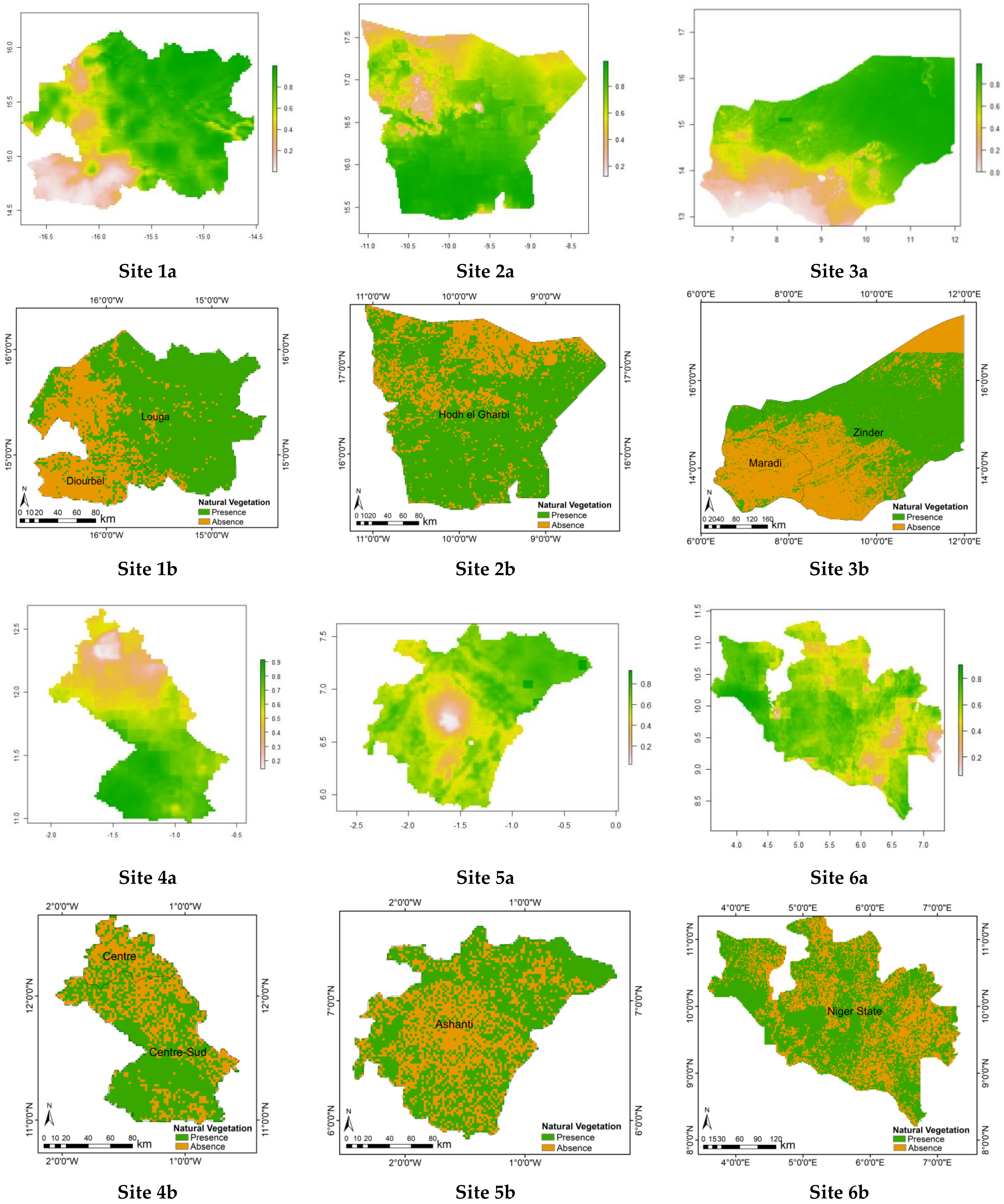
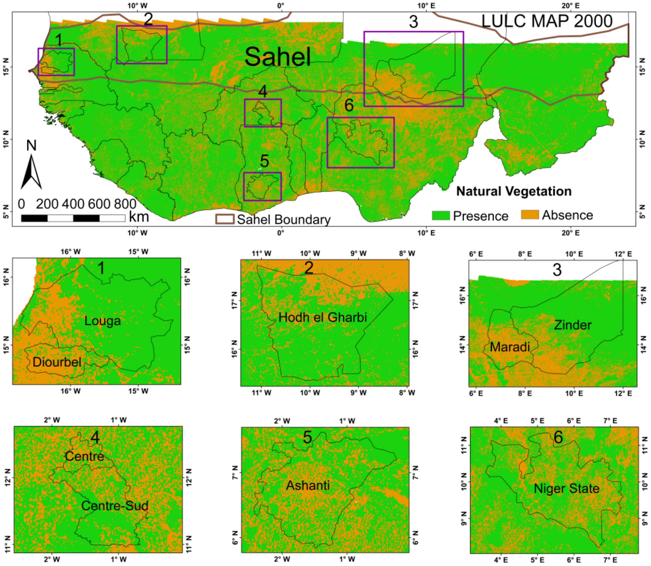
2.1. Study Area: Selected Hotspots in West Africa

The study was undertaken in West Africa. The area is characterized by five broad bio-climatic zones, i.e., Saharan, Sahelian, Sudanian, Guinean, and Guineo-Congolian [60]. These five broad bioclimatic zones were further categorized into two major bio-climatic zones on the basis of the wetness index defined as the ratio of mean annual precipitation (MAP)/mean annual potential evapo-transpiration (MAE) by Trabucco and Zomer [56]. Areas with MAP/MAE < 0.4 and MAP/MAE ≥ 0.4 were categorized as Sahel (arid-semi arid) and Sudanian, Guinean, and Guineo-Congolian (humid) regions, respectively, for the purpose of this study. The Saharan eco-region in West Africa was not included in this analysis due to the desert conditions [61]. For a description of the different LULC types and long-time dynamics in West Africa, we referred to Asenso Barnieh et al. [11]. Six sites with massive natural vegetation loss between 1975 and 2000 were selected for this analysis (see Figure 1). Three sites, i.e., Site 1. Diourbel-Louga (Senegal), Site 2. Hodh el Gharbi (Mauritania), and Site 3. Zinder-Maradi (Niger) were located in the arid regions and the remaining three sites were located in the humid region, i.e., Site 4. Centre and Centre Sud (Burkina Faso), Site 5. Ashanti region (Ghana), and Site 6. Niger State (Nigeria) of the study area.

2.1.1. Site 1: Diourbel-Louga (Senegal)

Diourbel-Louga is located in the Peanut Basin of Senegal within the Sahel (arid) region. The extent of the area is about 29,537.5 km⁻². The climate here is characterized by two major seasons, i.e., nine months of the dry season, i.e., October-June and three months of rainy season, i.e., July-September [62]. In the west, cropland fields were abandoned and replaced by grasslands and other vegetation since the 1980s. The land devoted to rain-fed crops remained fairly stable between 1975 and 2000 and agricultural expansion continued in the east. This overshadows the actual magnitude of rapid agricultural land increases in this region [11,61,63]. The major soil types in the area are Cambisols, Gleysols, Arenosols, Regosols, and Vertisols. Arenosols is the dominant soil type.

2.1.2. Site 2: Hodh el Gharbi (Mauritania)

Hodh el Gharbi is situated in the southern part of Mauritania and covers a land area of about 50,273 km⁻². The area falls within the Sahel region with very high inter-annual rainfall variability and is characterized by sandy dunes supporting large rangelands and comparatively fertile ferruginous soils with agricultural potential. The major soil types in the area are Lithosols, Luvisols, Arenosols, and Regosols. Here, steppe and Sahelian short grass savannah are the dominant vegetation types. Previous analyses of LULC transitions in this region revealed replacement of natural vegetation by other LULC types, such as bare land and sand dunes [11,61].

2.1.3. Site 3: Zinder-Maradi (Niger)

Zinder-Maradi is situated in the lowest part of the Niger Plateau in South-central Niger with Sahelian bioclimatic conditions characterized by a large inter-seasonal and intra-seasonal variability of rainfall, with annual rainfall between 200 and 600 mm a⁻¹ and accompanied by high temperatures in the dry season. The extent of the area is approximately 185,067 km⁻². The dominant soil types in the area are Arenosols, Gleysols Lithosols, Luvisols, Fluvisols, Vertisols, Regosols, and others [55]. The mean bio-productivity in this region increases toward the southern boundary of the country with relatively high population density between 80 and 150 inhabitants/people km⁻² coupled with “wall-to-wall” farmland, where agricultural fields occupy nearly the entire landscape [61]. Approximately 80% of all land is cultivated with few uncultivated natural vegetation patches, making the region the largest agricultural area in Niger. Here, farmers preserve trees by natural regeneration. This is a practice which has improved on-farm trees and crop production in the area. Farmers experienced major tree declines in the 1970s and 1980s as a result of drought, expanding cropland, and human pressure [64,65].

2.1.4. Site 4: Centre and Centre Sud (Burkina Faso)

Centre and Centre Sud are located in southern Burkina Faso across a wide bioclimatic gradient with annual rainfall between 650 mm a⁻¹ and 1000 mm a⁻¹ in the more humid Sudanian Region. The extent of the area is about 14,381 km⁻². Forest, gallery forest, Savanna, steppe, and rocky land are the major LULC types in the country. Previous LULC change analysis revealed the replacement of natural vegetation by cropland and settlements, along the Ouagadougou-Pama corridor in the southeast [11,61]. The major soil types in the area are Luvisols, Lithosols, Cambisols, Vertisols, Regosols, and Planosols.

2.1.5. Site 5: Ghana (Ashanti Region)

The Ashanti Region is located in the south-central part of Ghana where previous LULC transition analyses revealed massive natural vegetation loss due to encroachment by cropland and settlements. In the last four decades, the population density in Kumasi, which is Ghana’s second-largest city, has risen sharply due to substantial rural-urban migration led by the development of factories and business activities both in and around the city, thereby, exacerbating negative impacts on pristine forest reserves (e.g., Bobiri forest reserve and Banda Hills). The extent of the area is about 24,904.1 km⁻². The region is characterized by two rainy seasons, i.e., the major rainy season in April to August and the minor rainy season from September to November with mean annual rainfall of 1270 mm a⁻¹ [66]. The major soil types in the area are Acrisols, Lithosols, Nitosols, and Luvisols.

2.1.6. Site 6: Nigeria (Niger State)

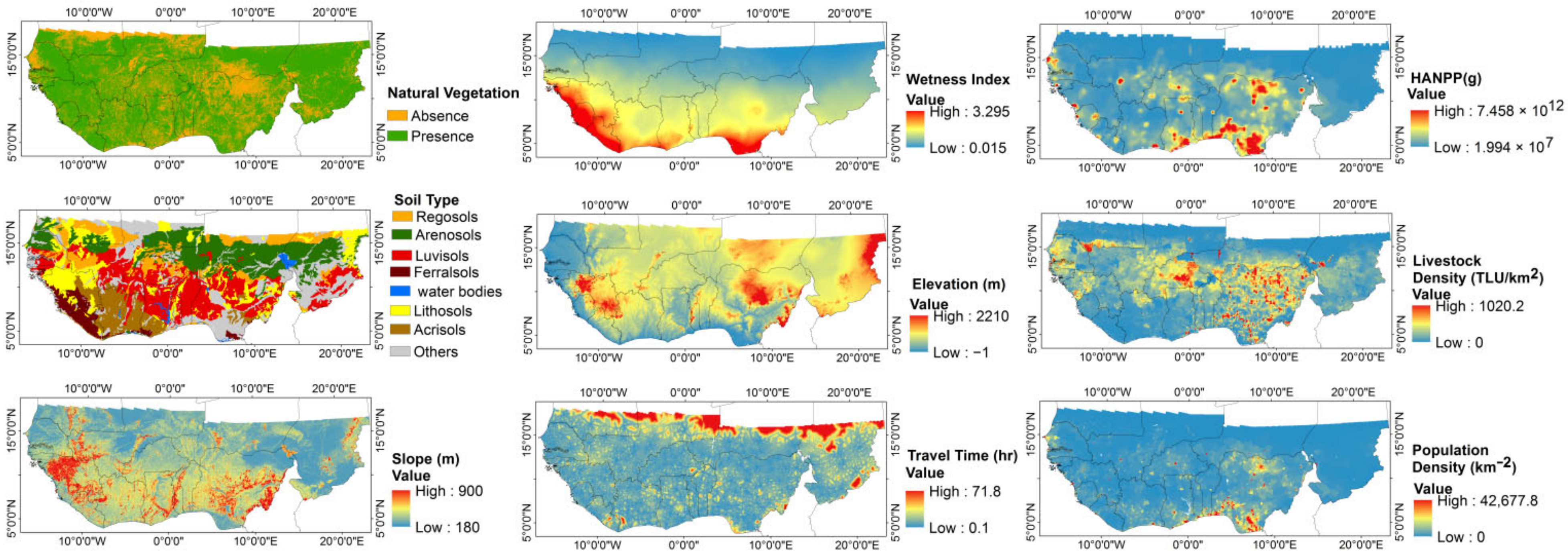
The Niger State is located at the Southern Guinea Savannah zone of Nigeria and extends into a land area of about 71,017.8 km⁻². Livestock rearing is prominent in this state. The state has a rainy season from April to October and a dry season from November to March. Mean relative humidity is 59% and temperature varies between 22 °C and 39 °C. The mean annual rainfall is between 1200 mm and 1300 mm a⁻¹, with the highest temperature in March and the lowest in August. The major soil types in the area are Nitisols, Luvisols, Lithosols, and Fluvisols. Previous LULC transition analyses in this region revealed settlement, rain-fed, and irrigated cropland, plantation, and open mines fields’ expansions at the expense of natural vegetation [11,61].

2.2. Datasets

The LULC map in 2000 was acquired from the United States Geographical Survey (USGS), West African Land Use Dynamic project. The data extend over seventeen countries in West Africa at 2 km spatial resolution. Only a small part of Cameroon was mapped. Additionally, according to CILSS [61], the northern parts of Mauritania, Mali, Niger, and Chad were not mapped due to the desert conditions, stable vegetation, and other LULC types (e.g., sand and rocks) through time. As a result, the unmapped northern parts of the previously mentioned countries, Cape Verde and Cameroon, were excluded from the analyses in this paper. The white regions on the map in Figure 1 are the areas without data and, therefore, were not mapped. Comprehensive definitions of the LULC types in the map can be found in a book published by CILSS [61]. The data was accessible at https://eros.usgs.gov/westafrica (accessed on 10 November 2018). The original LULC data with 24 classes had been re-classified into 7 LULC classes in a previous research study [11]. The reclassified map was further categorized into either presence or absence of natural vegetation and used as a dependent variable in a binary logistic regression (BLR) model we established in this study. To explain the spatial patterns and long-term response of natural vegetation to changes induced by the interplay of complex human-environmental interactions and other multiple drivers, perceived drivers of a LULC change in the study area were reviewed from literature and eight independent geospatial datasets of these perceived drivers were acquired from an open source earth observation database and categorized as: (a) natural/climate drivers, i.e., slope, elevation, soil type, and wetness index and (b) anthropic drivers, i.e., human appropriation of net primary productivity (HANPP), population density, livestock density, and accessibility drivers, i.e., travel time from natural vegetation areas to urban resources. Potential drivers without geospatial dimensions were excluded from the analyses because one of the major objectives of this study was to develop a spatially explicit dynamic model on independent predictive variables. The categorization was based on a conceptual framework developed from a combination of the Boserupian (1965), Malthusian (1826), Ricardian (1817), and von Thunen’s (1966) LULC change theories described by Chomitz and Gray [16] and Mazzucato et al. [22].

The soil map has information about the major soil groups of the world [55]. The spatial resolution of this dataset was about 10 km. Each grid cell contains the unique value that depicts the features of the major group it represents. The dataset is available at: http://www.fao.org:80/geonetwork/srv/en/resources.get?id=14129&fname=Map4_5.zip&access=private (accessed on 10 May 2018).

The global slope dataset was obtained from the United States Geographical Survey (USGSS). The gridded slope layer was mapped at about 1 km spatial resolution. The data and the metadata, which explains how the dataset was produced, can be accessed from https://www.usgs.gov/natural-hazards/earthquake-hazards/science/vs30-models-and-data (accessed on 10 May 2018). The elevation data was extracted from the Digital Elevation Model (DEM) data acquired by the NASA- Shuttle Radar Topography Mission (SRTM). The dataset is available for downloads at 30 m resolution at https://developers.google.com/earth-engine/datasets/catalog/USGS_SRTMGL1_003 (accessed on 10 May 2018). Figure 2 shows the LULC map and the geospatial datasets of the eight potential predictors we used for the analysis.

The wetness index gridded dataset was mapped at 1 km spatial resolution. This index is given as a function of precipitation, temperature, and potential evapo-transpiration. The global mean wetness index has been binned into hyper arid, arid, semi-arid, dry sub-humid, and humid (i.e., < 0.03, 0.03–0.2, 0.2–0.5, 0.5–0.65, >0.65), respectively [56]. Details of the method used to estimate the mean wetness index from 1950 to 2000 can be accessed from the CGIAR-CSI GeoPortal at: https://www.dropbox.com/sh/e5is592zafvovwf/AAAijCvHNiE4mYvYqWDpeJ3Ga/Global%20PET%20and%20Aridity%20Index?dl=0 (accessed on 10 May 2018)

A gridded raster map of accessibility (i.e., mean travel time (hours) from natural areas to the nearest town, market, other urban resources) and human settlements greater than 20,000 inhabitants was obtained from the FAO-Geo-network database. This dataset was generated by the Harvest Choice (2015) and available for downloads at http://harvestchoice.org/data/TT_20K (accessed on 10 May 2018).

The demography driving factors map (time series gridded population density map of West Africa at five-year intervals (from 1995–2000) was obtained from Center for International Earth Science Information Network CIESIN [67]. This dataset is a spatially explicit global population census data mapped at 1 km, which depicts the distribution of the human population in each grid cell. The dataset can be accessed at https://sedac.ciesin.columbia.edu/data/set/gpw-v4-population-density-adjusted-to-2015-unwpp-country-totals-rev11 (accessed on 10 May 2018).

The global patterns in human appropriation of net primary productivity (HANPP) have been mapped at 28 km spatial resolution in grams of carbon per grid cell. The datasets were downloaded from: http://sedac.ciesin.columbia.edu/es/hanpp.html (accessed on 25 January 2019). [57]. The gridded livestock density datasets were available at: http://harvestchoice.org/data/ad05_tlu (accessed on 24 February 2019). The datasets included livestock grazing and browsing values mapped at a 5 km spatial resolution as density of livestock per cell measured as tropical livestock units (TLU/sq. km). In addition, Google Earth Imagery and other ancillary data were also obtained for the validation of the results of the analyses.

Table 1. Summary of the datasets.

Variable	Sources	Spatial Resolution	Temporal Coverage
LULC raster map	USGS(2000)	2000 m	2000
Elevation	NASA-SRTM	30 m	Static
Slope	USGSS	1 km	Static
Soil Type	FAO GEONETWORK	10 km	Static
Wetness Index	CGIAR-CSI (1950–2000)	1 km	1950–2000
Travel Time	FAO GEONETWORK-Harvest Choice	10 km	Benchmarked 2000
Live Stock Density	FAO GEONETWORK-Harvest Choice	5 km	Benchmarked 2000
HANPP	SEDEC	28 km	1975–2000
Population Density	SEDEC	1 km	2000

USGS, NASA-SRTM, FAO, CGIAR-CSI, SEDEC, and HANPP represent United States Geographical Survey, National Aeronautics and Space Administration-Shuttle Radar Topography Mission (NASA-SRTM), Food and Agriculture Organization (FAO), Consultation Group for International Agricultural Research-Consortium for Spatial Information (CGIAR-CSI), Social and Economic Development Centre (SEDEC) and Human Appropriation of Net Primary productivity (HANPP) respectively.

is a summary of the datasets we used for the analysis.

3. Methodology

3.1. Binary Logistic Regression (BLR) Model

Nelder and Wedderburn [36] defined the BLR model as “empirically parameterized static model that compute probabilities, which indicate the likelihood of the occurrence of a specific event at a specific location in time.” The BLR approach can model the inherent complex human environmental interactions to inform a LULC change. Where this change occurs over a longer period of time, the underlying drivers of change and how these drivers interact with the LULC system. The probability that a given LULC type (Y) is equal to (1), i.e., present for a given value of X or a change in a time-dependent variable can be determined by a BLR model. In a situation whereby the BLR model is generated by geospatial datasets, the technique yields coefficients that can be used to generate maps of the probability of occurrence of events, which is, in our case, the presence of natural vegetation [30,68]. Therefore, based on the BLR model and the potential predictors we used in this study, the probability P of observing the presence (1) or absence (0) of natural vegetation in a given pixel in the year 2000 can be expressed as:

$$P\left(\mathrm{Presence}\mathrm{of}\mathrm{Natural}\mathrm{Vegetation}\right)=\frac{Ex{p}^{{\mathsf{\beta }}_0+{\mathsf{\beta }}_1\mathrm{Mean}\mathrm{Wetness}\mathrm{index}+{\mathsf{\beta }}_2\mathrm{Mean}\mathrm{HANPP}\dots +{\mathsf{\beta }}_{\mathrm{n}}{\mathrm{x}}_{\mathrm{n}}+e}}{1+Ex{p}^{{\mathsf{\beta }}_0+{\mathsf{\beta }}_1\mathrm{Mean}\mathrm{Wetness}\mathrm{index}+{\mathsf{\beta }}_2\mathrm{Mean}\mathrm{HANPP}\dots +{\mathsf{\beta }}_{\mathrm{n}}{\mathrm{x}}_{\mathrm{n}}+e}}$$

(1)

where ${\mathsf{\beta }}_0$ stands for the intercept, ${\mathsf{\beta }}_1$, ${\mathsf{\beta }}_2$ $\dots {\mathsf{\beta }}_{\mathrm{n}}$ are the slope parameters, and $\left\{{\mathrm{x}}_{1,} {\mathrm{x}}_{2,}\dots ,{\mathrm{x}}_{\mathrm{n},}\right\}$ are the vectors of the independent predictors per grid cell. In this study, the predictors were: wetness index, HANPP, travel time, livestock density, population density, soil type, elevation and “slope”, and $e$ is the residual [44,52,69]. The detailed methodology is explained in Section 3.2 through Section 3.5. The output of the BLR model can be interpreted to rank the importance of the drivers. The ranking of the predictors shows which driver has the greatest effect on the dependent variable. The BLR also yields an estimate of the significance of the drivers. In regression analyses, the probability that the observed relationship between the independent and the dependent variable occurs by chance gives the statistical significance level. The statistical significance level is inversely proportional to the set confidence level, i.e., the smaller the statistical significance, the higher the confidence of the relationship between the variables under consideration [34]. In this study, the statistical p-value was applied as a metric of significance of the multiple set of predictors, while the absolute value of the standardized BLR model coefficients and the odds ratio were used to determine and rank the importance of the drivers. The odds of an event are given by $P/\left(1-P\right)$, where $P$ is the probability that the event will occur. The odds ratio is defined as the ratio of two odds and accounts for the effects of an independent variable on the dependent variable. The odds ratio is calculated as:

$$\mathrm{OR}=\frac{\raisebox{1ex}{$P\left(\mathrm{event}|\mathrm{x}+1\right)$}\!\left/ \!\raisebox{-1ex}{$\left(1-P\left(\mathrm{event}|\mathrm{x}+1\right)\right.$}\right.}{\raisebox{1ex}{$P\left(\mathrm{event}|\mathrm{x}\right)$}\!\left/ \!\raisebox{-1ex}{$\left(1-P\left(\mathrm{event}|\mathrm{x}\right)\right.$}\right.}$$

(2)

The natural log of the odds ratio gives the logit coefficient, i.e., the exponent β (${\mathrm{Exp}}^{\mathsf{\beta }}$) in Equation (1). Therefore, the two functions are a measure of the same effect (i.e., the strength of the relationship between the dependent variable, and the independent predictors) [44,51]. Lower odds of an event will give $\mathsf{\beta }<0,{\mathrm{Exp}}^{\mathsf{\beta }}<1$, while higher odds will give $\mathsf{\beta }>0, {\mathrm{Exp}}^{\mathsf{\beta }}>$1. The major reason for choosing the BLR model for our analysis is its ability to accommodate a wide range of data types, i.e., categorical (binary, ordinal) and continuous data, which are typical examples of data types employed in LULC modeling. On top of it, if the objective is to predict the probability of an event, the BLR model can be optimized to achieve better prediction accuracy unlike the other “black box” models [44]. To develop the BLR model, five steps were followed (i.e., literature review on potential drivers (see Introduction), geospatial data acquisition and preparation, multi-collinearity analysis, BLR model development, and validation).

3.2. Data Preparation

One of the ways to model the relationship in space and time between the presence of a given LULC type and multiple predictors at the continental scale is to determine historical changes in LULC for the whole continent in order to identify hotpots of severe changes. Spatially explicit dynamic models may then be developed to relate the observed LULC type in each hotspot to multiple predictors, e.g., factors that determine the presence of natural vegetation. In this way, the dominant underlying drivers at the continental scale can be captured. In the case of this study, long time LULC transitions mapping and hotspots identification in the study area, i.e., West Africa had been undertaken by Asenso Barnieh et al. [11]. Natural vegetation (forestland and other natural vegetation) encroachment by other LULC types, i.e., cropland, wetland, water bodies, settlements, and other LULC were the major transitions detected between 1975 and 2000. Therefore, this study focused on understanding the underlying drivers, which determined the presence of natural vegetation at some of the selected hotpots in West Africa. Due to geospatial data gaps on the potential drivers after 2000, we restricted our analysis to the years prior to 2000. However, the approach we used can be applied to model occurrence of natural vegetation at any given year when data availability is not a limiting factor.

On the basis of the previously mentioned BLR modeling approach [37], the observed LULC map of a given year (2000) with 7 LULC classes (cropland, forestland, other vegetation, wetland, water, settlement, and other LULC types) developed by Asenso Barnieh et al. [11] was further aggregated into just two categories, i.e., presence of natural vegetation, i.e., forestland and other natural vegetation and absence of natural vegetation, i.e., cropland, wetland, water bodies, settlements, and other LULC types. These major LULC categories were converted into a binary dataset and coded as 1 (presence of natural vegetation) and 0 (absence of natural vegetation). The binary LULC map and all the other geospatial gridded raster maps of the potential drivers were projected and resampled to the same spatial resolution (2 km) as the LULC map in 2000. This analysis was conducted in ARCGIS version 10.4 and the results were exported into R computing programming software interface for further analysis. All the missing values in the entire datasets were removed [44]. The datasets were divided into training (80%) and testing (20%) for the development of the model and validation, respectively. In order to examine the range of values of the potential drivers, the individual datasets were plotted against the natural vegetation dataset.

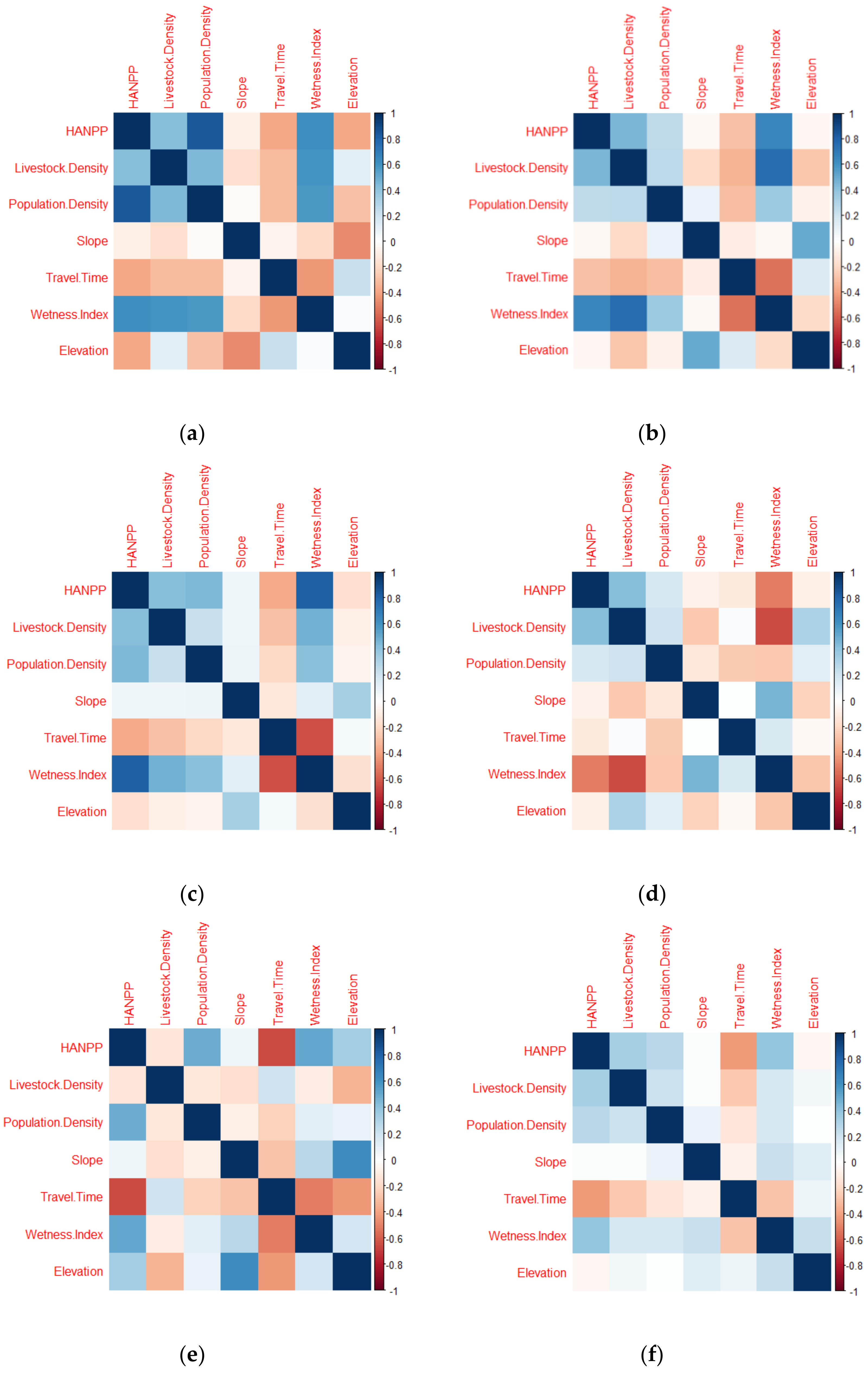
3.3. Multi-Collinearity Analysis

Collinearity occurs in multiple regressions modeling when any of the predictors are strongly correlated and two or more of the predictors bring the same information into the model. Strongly correlated predictors may inflate the standard errors of the regression coefficients in multi-variant regression and reduce the power of the significance test [44]. To identify the predictor variables, which may exhibit multi-collinearity and to remove redundant variables from the model, we analyzed correlation of the predictor variables after re-sampling the data to the same spatial resolution (2 km, i.e., the spatial resolution of the observed LULC map). Apart from the correlation analysis, other means of multi-collinearity analysis (variance inflation factor (VIF), kappa, and conditional number of the eigen values) were also employed. While the output from the correlation matrix was used to examine the kappa and the conditional numbers of the eigen-values in the model, the output from the BLR model fitted with all the potential drivers was used to examine the VIF of these drivers. Any driver with VIF greater than 10 indicates severe multi-collinearity in the model. In addition, kappa and conditional numbers of the eigen-values greater than 100 indicate severe multi-collinearity [40,51,70,71].

3.4. Model Development

The presence of natural vegetation, i.e., P(Y) for a given set of values of the independent predictors X was modeled by fitting a BLR. The previously mentioned potential drivers, i.e., mean wetness index, mean population density, soil type, elevation, and travel time from natural areas to urban resources, livestock density, and HANPP (Section 3.2) were used to develop the BLR model. The BLR model calculates the natural logarithm of the odds ratio (the probability of occurrence against the probability of non-occurrence of an event) to transform a non-linear model into a linear model [72]. The development of the BLR model was based on Equation (1).

The output of this model ranks the contribution of each variable in explaining the presence of natural vegetation. Prior to the binary logistic modeling with the multiple predictors, a one-to-one logistic regression model was initially fitted between the binary response LULC data and each predictor. The rationale was to exclude insignificant drivers before the development of the multivariate BLR model. The model was run stepwise in a forward and backward direction to eliminate redundant variables, which may exhibit multi-collinearity in order to remove less significant variables.

The most important drivers of natural vegetation’s occurrence were determined based on Wald Statistics and the odds ratio from the BLR model. The variable with the highest standardized coefficient was the most important in explaining occurrence of natural vegetation in 2000. To determine the dominant categories of drivers, i.e., natural or anthropic activities in each study site, the BLR model was again determined first using natural predictors only, i.e., slope, elevation, soil type, and wetness index, and second human influence predictors only, i.e., a combination of anthropic (i.e., HANPP, livestock density) and accessibility indicator, i.e., travel time. The rationale was to ascertain which of the two combinations would provide a better BLR model fit.

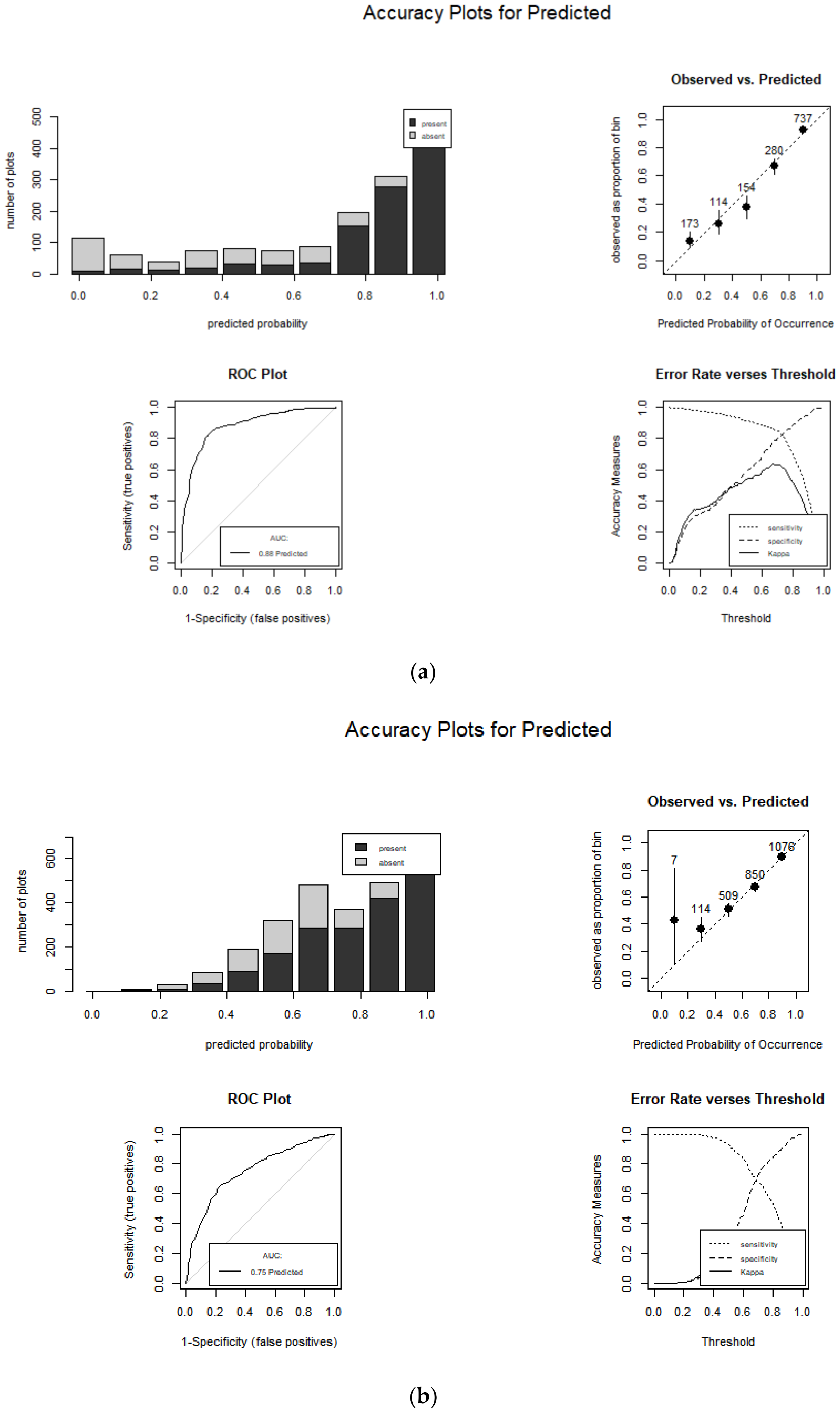
3.5. Model Validation

Data-splitting was adopted to validate the BLR model. Prior to the BLR modeling, the total observations in each hotspot were randomly divided into two sets, i.e., training samples of 80% (model development) and testing samples of 20% (model evaluation). The Akaike information criterion (AIC), Bayesian information criterion (BIC), and log likelihood-ratio were used as metrics for two or more model evaluations. Stepwise forward selection of the most significant predictors and backward elimination of the least significant predictors were applied in this evaluation. If two selection criteria give the same results, then multi-collinearity in the model can be neglected [34,51,73,74,75,76,77,78].

The entire stepwise selection technique was an iterative process. In the case of the forward selection process, the model was initially fitted with the most significant predictors and additional predictors were added in order of significance. The iteration stops when no improvement can be achieved by including additional predictors. By contrast, the stepwise backward selection process is initialized by fitting the model with all the possible predictors and eliminates the least significant one at each step until the decrease in model accuracy at each step is less than a pre-set threshold. At each stage of both forward and backward selection, AIC, p-values, and the residual, with the number of degrees of freedom being the number of the independent predictors remaining at each stage, were used to set a termination rule. Lower AIC, p-values, Log likelihood ratios, and residual deviance were used to determine the best fitted model. A p-value < 0.05 was considered as the optimal termination rule to include significant variables [34,51,73,74,75,76,77,78].

The ability of the BLR model to predict the presence of natural vegetation was evaluated with the testing samples. Using Equation (1) and the BLR model coefficients estimated with the training samples, we predicted the presence of natural vegetation in each hotspot of the study area. The AUC, which is the area under the receiver operating characteristics (ROC) curve, was used to evaluate the predictive accuracy of the BLR model [47,70,71,76,79,80,81]. The true positive rate of the predicted values was plotted against the false positive rate at various threshold settings [68]. The AUC ranges from 0 to 1. AUC less than or equal to 0.5 is an indication that the model prediction is random, while AUC > 0.5 indicates a deterministic prediction of the response variable. AUC ≈ 1 is an indication of a perfect fit [47,70,71,76,79,80,81]. The map of predicted probabilities for the presence of natural vegetation in each hotspot site was compared with the observed map as a means of additional validation.

4. Results

4.1. Multi-Collinearity

The descriptive (

Table 2. Descriptive statistics of the continuous predictor variables at the various study sites in West Africa at a grid cell of 2 km spatial resolution.

Study Sites	Variables	Mean	SD	Median	Minimum	Maximum	Range	Skew	Kurtosis	SE
1. Diourbel-Louga, Senegal	HANPP (g)	8.94 × 1010	1.03 × 1011	4.15 × 1010	1.05 × 1010	4.89 × 1011	4.78 × 1011	1.53	1.25	1.27 × 109
Number of Samples = 6557	Livestock Density (TLU/km2)	26.19	8.64	25.40	0.20	96.25	96.05	0.47	3.08	0.11
	Population Density (people km−2)	57.73	79.92	11.58	2.55	308.24	305.69	2.14	3.59	0.99
	Slope (m)	251.71	37.02	237.91	203.81	583.57	379.76	2.47	9.55	0.46
	Travel Time (hr)	2.60	1.17	2.38	0.17	10.27	10.10	1.63	4.60	0.01
	Wetness Index	0.20	0.03	0.20	0.13	0.28	0.15	0.20	−0.37	0.00
	Elevation (m)	40.96	11.28	43.86	2.52	60.64	58.13	−0.85	−0.05	0.14
2. Hodh el Gharbi	HANPP (g)	6.39 × 109	5.82 × 109	5.15 × 109	8.58 × 108	6.37 × 1010	6.29 × 1010	4.82	2.85 × 101	5.42 × 107
Number of Samples = 11,498	Livestock Density (TLU/km2)	10.43	13.64	2.49	0.00	57.30	57.30	1.29	0.47	0.13
	Population Density (people km−2)	4.55	6.72	3.97	0.11	114.77	114.65	9.49	127.97	0.06
	Slope (m)	327.46	119.27	290.00	205.20	899.99	694.79	2.17	5.11	1.11
	Travel Time (hr)	7.86	4.22	6.47	1.62	23.66	22.04	1.41	1.49	0.04
	Wetness Index	0.11	0.03	0.10	0.06	0.21	0.15	0.84	0.30	0.00
	Elevation (m)	213.22	44.44	201.50	140.13	444.44	304.31	1.68	3.68	0.41
3. Zinder-Maradi, Niger	HANPP (g)	4.52 × 1010	5.59 × 1010	1.41 × 1010	3.00 × 109	3.49 × 1011	3.46 × 1011	1.55	2.05	2.82 × 108
Number of Samples = 39,277	Livestock Density (TLU/km2)	14.23	23.06	10.00	0.00	526.20	526.20	14.93	315.94	0.12
	Population Density (people km−2)	25.22	64.95	9.66	0.22	2593.00	2592.78	20.87	593.26	0.33
	Slope (m)	299.47	80.40	280.15	200.36	896.25	695.88	2.70	10.71	0.41
	Travel Time (hr)	6.70	8.11	3.48	0.29	48.13	47.84	2.44	5.74	0.04
	Wetness Index	0.11	0.06	0.12	0.02	0.29	0.27	0.17	−0.85	0.00
	Elevation (m)	428.74	43.17	430.33	304.08	603.33	299.24	0.02	−0.45	0.22
4. Centre-Centre Sud, Burkina Faso	HANPP (g)	1.72 × 1011	1.20 × 1011	1.44 × 1011	2.38 × 1010	8.18 × 1011	7.94 × 1011	1.77	4.67	2.14 × 1019
Number of Samples = 3155	Livestock Density (TLU/km2)	51.13	24.15	49.40	0.00	108.90	108.90	0.09	−0.80	0.43
	Population Density (people km−2)	119.08	312.64	55.93	6.93	1886.85	1879.91	4.98	23.99	5.57
	Slope (m)	343.12	43.10	335.39	254.52	734.40	479.89	2.76	14.67	0.77
	Travel Time (hr)	2.75	1.56	2.29	0.18	8.78	8.61	1.38	1.87	0.03
	Wetness Index	0.42	0.03	0.42	0.36	0.50	0.15	0.44	−0.82	0.00
	Elevation (m)	293.25	26.19	295.44	205.57	356.24	150.67	−0.41	−0.08	0.47
5. Ashanti Region, Ghana	HANPP (g)	2.14 × 1011	1.19 × 1011	2.01 × 1011	5.26 × 1010	8.13 × 1011	7.60 × 1011	1.26	2.54	1.62 × 109
Number of Samples = 5456	Livestock density (TLU/km2)	5.39	1.88	5.27	0.00	12.90	12.90	0.32	0.08	0.03
	Population density (people km−2)	153.47	456.63	83.25	17.07	4849.50	4832.42	8.61	78.17	6.18
	Slope (m)	493.16	157.32	436.65	261.99	900.00	638.01	1.01	−0.08	2.13
	Travel time (hr)	3.52	2.49	2.74	0.12	14.36	14.24	1.52	1.78	0.03
	Wetness index	0.84	0.09	0.84	0.69	1.06	0.37	0.18	−1.11	0.00
	Elevation (m)	221.80	83.85	211.26	77.43	625.99	548.56	0.87	0.78	1.14
6. Niger State, Nigeria	HANPP (g)	6.25 × 1010	2.85 × 1010	6.03 × 1010	1.72 × 1010	1.70 × 1011	1.53 × 1011	7.05 × 10−1	4.16 × 10−1	2.27 × 108
Number of Samples = 15,731	Livestock density (TLU/km2)	19.85	14.43	17.10	0.00	94.00	94.00	1.45	3.14	0.12
	Population density (people km−2)	47.35	103.52	38.77	14.16	3117.93	3103.77	17.70	373.64	0.83
	Slope (m)	465.36	111.76	445.55	200.10	900.00	699.90	0.91	1.24	0.89
	Travel time (hr)	3.75	2.65	2.97	0.11	20.61	20.49	2.74	10.14	0.02
	Wetness index	0.61	0.05	0.62	0.49	0.76	0.27	0.05	0.41	0.00
	Elevation (m)	250.28	107.31	244.83	44.56	620.58	576.02	0.48	−0.10	0.86

Here, SD, SE, TLU, and HANPP represent standard deviation (SD), standard error (SE), tropical livestock unit (TLU), and human appropriation of net primary productivity (HANPP), respectively.

) statistics illustrate the patterns in the variables we used for the development of the BLR model. The mean HANPP (2.14 × 10¹¹, 1.728 × 10¹¹, 8.94 × 10¹⁰ and 26.25 × 10¹⁰ in grams of carbon) was relatively higher in the Ashanti Region of Ghana, Centre-Centre Sud of Burkina Faso, Diourbel-Louga in Senegal, and Niger State in Nigeria coupled with a denser population, i.e., mean population densities of 153.47, 119.08, 57.73, and 47.35 inhabitants/people km⁻², respectively. Except Diourbel-Louga in Senegal, the mean wetness indexes, i.e., 0.84, 0.42, 0.20, and 0.61 in the previously mentioned areas were comparatively high, thus, placing these regions in the humid agro-ecological zone as defined in Section 2.2. Overall, livestock density did not appear to correlate with population density across the sub-continent since the mean population density in some study sites, e.g., Ashanti Region of Ghana, was comparatively high when coupled with low mean livestock density (Table 2). Comparatively, the mean travel time, i.e., 3.52, 2.75, 2.60, and 3.74 hr to grid cells endowed with urban resources was lower in densely populated sites, i.e., Ashanti Region of Ghana, Centre-Centre-Sud, in Burkina Faso, Diourbel in Senegal, and Niger State in Nigeria, than in sparsely populated sites, i.e., Zinder-Maradi in Niger and Hodh el Gharbi in Mauritania, where it was 6.70 and 7.86 hr, respectively.

Figure 3 shows the pairwise correlation between the continuous predictor variables at the various study sites.

Table 3. The binary logistic regression (BLR) model output summary. HANPP represents human appropriation of net primary productivity.

Arid Region
Study Sites	Variables	Parameter Estimate β	Standard Error	Wald (Z Value)	Pr(>│Z│)	Significance Codes
1. Diourbel-Louga, Senegal	Intercept	−1.150	6.200 × 10−1	−1.845	6.500 × 10−2	•
Number of Samples = 6557	HANPP	−9.162 × 10−12	7.512 × 10−13	−1.220 × 101	2.000 × 10−16	***
Training = 5099	Travel Time	6.626 × 10−1	5.126 × 10−2	1.293 × 10	2.000 × 10−16	***
Testing = 1458	Slope	1.057 × 10−2	1.545 × 10−3	6.840	7.940 × 10−12	***
Area Under the ROC/AUC	Livestock Density	−2.878 × 10−2	5.103 × 10−3	−5.639	1.710 × 10−8	***
Climate Drivers = 0.83	Elevation	3.659 × 10−2	5.087 × 10−3	7.193	6.320× 10−13	***
Human Drivers = 0.87	Soil Type	1.949 × 10−2	5.878 × 10−3	3.316	9.130 × 10−4	***
Climate and Human = 0.88	Wetness Index	−1.187 × 101	2.256	−5.263	1.420 × 10−7	***
	Population Density	2.046 × 10−3	8.291 × 10−4	2.468	1.358 × 10−2	*
2. Hodh el Gharbi, Mauritania	Intercept	2.977	3.423 × 10−1	8.698	2.000 × 10−16	***
Number of Samples 11,408	Livestock Density	2.965 × 10−2	4.116 ×10−3	7.205	5.820 × 10−13	***
Training Samples = 8942	Elevation	−9.042 × 10−3	7.009 × 10−4	−1.290 × 101	2.000 × 10−16	***
Testing Samples = 2556	Wetness Index	2.008 × 101	2.216	9.063	2.000 × 10−16	***
Area Under the ROC/AUC	HANPP	−5.577 × 10−11	6.688 × 10−12	−8.338	2.000 × 10−16	***
Climate Drivers = 0.74	Slope	−2.113 × 10−3	2.530 × 10−4	−8.353	2.000 × 10−16	***
Human Drivers = 0.71	Soil Type	−5.705 × 10−2	8.708 × 10−3	−6.551	5.700 × 10−11	***
Climate and Human = 0.75	Travel Time	−4.374 × 10−2	7.004 ×10−3	−6.245	4.240 × 10−10	***
	Population Density	−2.104 × 10−2	4.141 × 10−3	−5.081	3.750 × 10−7	***
3. Zinder-Maradi, Niger	Intercept	6.035	2.276 × 10−1	2.651 × 10	2.00 × 10−16	***
Number of Samples = 39,277	Wetness Index	−2.250 × 101	7.572 × 10−1	−2.972 × 101	2.000 × 10−16	***
Training Samples = 30,549	Population Density	−1.382 × 10−2	1.042 × 10−3	−1.326 × 101	2.000 × 10−16	***
Testing Samples = 8728	Slope	−3.063 × 10−3	1.923 × 10−4	−1.593 × 101	2.000 × 10−16	***
Area Under the ROC/AUC	Travel Time	−3.527 × 10−2	3.264 × 10−3	−1.081 × 101	2.000 × 10−16	***
Climate Drivers = 0.86	HANPP	−4.768 × 10−12	6.011 × 10−13	−7.932	2.150 × 10−15	***
Human Drivers = 0.87	Soil Type	−2.089 × 10−2	4.910 × 10−3	−4.255	2.090 × 10−5	***
Climate and Human = 0.88	Livestock Density	5.008 × 10−3	1.585 × 10−3	3.159	1.583 × 10−3	**
	DEM	−1.498 × 10−3	4.078 × 10−4	−3.674	2.390 × 10−4	***
Humid Region
4. Centre-Centre Sud, Burkina Faso	Intercept	−1.761	1.255	−1.403	1.606 × 10−1
Number of Samples = 3155	Wetness Index	1.277 × 10	2.433	5.247	1.550 × 10−7	***
Training Samples = 2453	Livestock Density	−1.290 × 10−2	2.555 × 10−3	−5.050	4.430 × 10−7	***
Testing Samples = 702	Population Density	−5.907 × 10−4	1.701 × 10−4	−3.473	5.160 × 10−4	***
Area Under the ROC/AUC	HANPP	−1.546 × 10−12	4.601 × 10−13	−3.359	7.810 × 10−4	***
Climate Drivers = 0.70	Elevation	−4.879 × 10−3	1.888 × 10−3	−2.585	9.751 × 10−3	**
Human Drivers = 0.71	Slope	−2.376 × 10−3	1.212 × 10−3	−1.960	4.995 × 10−2	*
Climate and Human = 0.72	Travel Time	4.854 × 10−2	3.027 × 10−2	1.603	1.089 × 10−1
5.Ashanti Region, Ghana	Intercept	−8.415 × 10−2	2.295 × 10−1	−3.670×10−1	7.139 × 10−1
Number of Samples = 5456	HANPP	−3.001 × 10−12	4.520 × 10−13	−6.639	3.170 × 10−11	***
Training Samples = 4243	Slope	1.947 × 10−3	2.850 × 10−4	6.832	8.380 × 10−12	***
Testing Samples = 1213	Travel Time	7.631 × 10−2	1.997 × 10−2	3.821	1.330 × 10−4	***
Area Under the ROC/AUC	Elevation	−1.388 × 10−3	5.701 × 10−4	−2.435	1.489 × 10−2	*
Climate Drivers = 0.64	Population Density	−3.783 × 10−4	1.574 × 10−4	−2.403	1.626 × 10−2	*
Human Drivers = 0.66	Soil Type	−1.329 × 10−3	5.089 × 10−4	−2.611	9.038 × 10−3	**
Climate and Human = 0.70	Livestock Density	4.529 × 10−2	1.893 × 10−2	2.393	1.671 × 10−2	*
6. Niger State, Nigeria	Intercept	7.181 × 10−1	1.164 × 10−1	6.168	6.910 × 10−10	***
Number of Samples 15,731	Livestock Density	−2.247 × 10−2	1.471 × 10−3	−1.528 × 101	2.000 × 10−16	***
Training Samples = 12,235	HANPP	−8.350 × 10−12	7.862 × 10−13	−1.062 × 101	2.000 × 10−16	***
Testing Samples = 3496	Slope	1.660 × 10−3	1.791 × 10−4	9.267	2.000 × 10−16	***
Area Under the ROC/AUC	Travel Time	6.759 ×1 0−2	9.492 × 10−3	7.121	1.070 × 10−12	***
Climate Drivers = 0.57	Elevation	−1.173 × 10−3	1.819 × 10−4	−6.449	1.130 × 10−10	***
Human Drivers = 0.63	Soil Type	8.765 × 10−4	2.307 × 10−4	3.799	1.450 × 10−4	***
Climate and Human = 0.65	Population Density	−4.071 × 10−4	2.129 × 10−4	−1.912	5.585 × 10−2	•
Significance. Codes	p < 0.001 ***	p < 0.01 **	p < 0.05 *	p < 0.1 •	1

In each study site, the variables are arranged in order of significance. Insignificant variables were automatically removed by the algorithm used to develop the model. In some cases, some predictors were insignificant but were retained in the model if the removal would decrease the model accuracy. The predictors were ranked as follows: p < 0.001 *** (Extremely Significant), p < 0.01 ** (Very Significant), p < 0.05 * (Significant) p < 0.1 •(Less Significant), 1 (Insignificant). Here, AUC/ROC represents the area under the receiver operating characteristics (ROC) curve. The AUC ranges from 0 to 1. AUC less than or equal to 0.5 is an indication that the model prediction is random, while AUC > 0.5 indicates a deterministic prediction of the response variable. AUC ≈ 1 is an indication of a perfect fit.

is the BLR model output which shows the significance levels of the predictor variables and

Table 4. Model Performance Parameters.

Study Sites	Continuous Variables	VIF (Full Model)	Eigen Values
1. Diourbel-Louga-Senegal	Elevation	16.8	0.1
AIC = 4255.4	Slope	16.1	0.6
BIC = 4314.2	Wetness Index	20.6	0.3
Log Likelihood = −2118.7	Travel Time	18.6	0.4
Deviance = 4247.4	Live Stock Density	9.9	1.7
Training samples = 5099.0	HANPP	30.4	3.1
Kappa and Conditional Number = 23.5	Population Density	22.4	0.8
2. Hodh el Gharbi, Mauritania	Elevation	8.7	0.2
AIC = 8935.7	Slope	8.1	0.7
BIC = 8999.6	Wetness Index	39.1	0.4
Log Likelihood = −4458.9	Travel Time	7.8	0.5
Deviance = 8917.7	Live Stock Density	28	1.5
Training Samples = 8942.0	HANPP	13.5	2.8
kappa and Conditional Number = 17.9	Population Density	6.6	0.9
3. Zinder-Maradi, Niger	Elevation	9.4	0.1
AIC = 27,333.9	Slope	7.2	0.7
BIC = 27,408.9	Wetness Index	58.6	0.5
Log Likelihood = −13,658.0	Travel Time	21.4	0.6
Deviance = 27,315.9	Live Stock Density	40.5	1.3
Training Samples = 30,549.0	HANPP	34.5	2.9
Kappa and conditional Number = 24.4	Population Density	145.8	0.8
4.Centre-Cente-Sud, Burkina Faso	Elevation	6.1	0.3
AIC = 2988.6	Slope	7.2	0.8
BIC = 2980.1	Wetness Index	15.1	0.4
Log Likelihood = −1458.8	Travel Time	5.5	0.7
Deviance = 2917.6	Live Stock Density	9.4	1.2
Training Samples = 2453	HANPP	7.9	2.5
Kappa and conditional Number = 10.1	Population Density	6.9	1.1
5. Ashanti Region, Ghana	Elevation	10.6	0.2
AIC = 5366.5	Slope	9.5	0.7
BIC = 5417.3	Wetness Index	7.5	0.5
Log Likelihood = −2675.2	Travel Time	10.9	0.3
Deviance = 5350.5	Live Stock Density	5.4	1.4
Training Samples = 4243.0	HANPP	14.4	2.8
Kappa and conditional Number = 13.9	Population Density	21.9	0.9
6.Niger State, Nigeria	Elevation	4.9	0.5
AIC = 15,426.0	Slope	5.1	0.9
BIC = 15,485.3	Wetness Index	6.0	0.6
Log Likelihood = −7705.0	Travel Time	7.9	0.8
Deviance = 15,409.9	Live Stock Density	5.5	1.3
Training Samples = 12,235.0	HANPP	6.7	2.1
Kappa and conditional Number = 4.6	Population Density	6.5	0.9

Here, AIC, BIC, VIF, and HANPP represent Akaike information criterion (AIC), Bayesian information criterion (BIC), variance inflation factor (VIF), and human appropriation of net primary productivity, respectively.

shows the performance parameters of the model. In many of the sites analyzed, some drivers exhibited multi-collinearity (Figure 3 and Table 4). The correlation matrices (Figure 3) and the VIF of the full model (Table 4) indicated multi-collinearity in the model at Zinder-Maradi-Niger (HANPP and wetness index, correlation = 0.8) and Diourbel-Louga, Senegal (HANPP and Population density, correlation = 0.8) sites. The strength of the correlation did not exceed the threshold for severe collinearity (correlation value > 0.8) we set in this study. In both cases, the variables exhibited positive correlation. The VIF values suggested multi-collinearity in the full model, particularly in the study sites in the arid and semi-arid regions. The conditional number of the eigen values and the Kappa of the predictors did not exceed the thresholds, i.e., kappa and conditional number of the eigen values > 100, that we set for this study (Table 4). In general, multi-collinearity was an issue in the sites where the independent predictors could explain the presence of natural vegetation, regardless of the other predictors. If two collinear predictors bring the same information into the model, the internal algorithms of the BLR model remove the less important predictor.

4.2. Significant Underlying Drivers of Natural Vegetation Identified from the Binary Logistic Regresion (BLR) Model

The BLR model revealed that the occurrence of natural vegetation in West African landscape is determined by multiple combinations of drivers (Table 3 and

Table 5. The summary of the significance levels and the impacts of the underlying drivers on natural vegetation at some selected hotspots in West Africa.

Study Sites	Underlying Driving Factors
West Africa	HANPP	Pop. Density	L. Density	Travel Time	Slope	Elevation	Soil Type	W. Index
1. Diourbel-Louga, Senegal	Negative ***	Positive *	Negative ***	Positive ***	Positive ***	Positive ***	Positive ***	Negative ***
2. Hodh el Gharbi, Mauritania	Negative ***	Negative ****	Positive ***	Negative ***	Negative ***	Negative ***	Negative ***	Positive ***
3. Zinder-Maradi, Niger	Negative ***	Negative****	Positive **	Negative ***	Negative ***	Negative ***	Negative ***	Negative ***
4. Centre-Centre-Sud, Burkina Faso	Negative ***	Negative****	Negative ***	Insignificant	Negative *	Negative **	Insignificant	Positive ***
5. Ashanti Region, Ghana	Negative ***	Negative *	Positive *	Positive ***	Positive ***	Negative *	Negative **	Insignificant
6. Niger State, Nigeria	Negative ***	Negative •	Negative ***	Positive ***	Positive ***	Negative ***	Positive ***	Insignificant

Where, HANPP represents (Human Appropriation of Net Primary Productivity), Pop. Density (Population Density), L. Density (Livestock Density), and W. Index (Wetness Index). The “Negative” indicates that increasing the effect of the underlying drivers will decrease the presence of natural vegetation and vice versa. The “Positive” indicates that increasing the effect of the underlying drivers will increase the presence of natural vegetation. The predictors were ranked as follows: p < 0.001 *** (Extremely Significant), p < 0.01 ** (Very Significant), p < 0.05 * (Significant), p < 0.1 •(Less Significant), 1 (Insignificant). The shaded entries are the dominant underlying drivers and their significance impacts at each site.

). The combinations varied from one location to another, apparently responding to the local environmental and socio-economic conditions. The ranking of the drivers also differed from one location to another. Human influence predictors were the most significant in the Ashanti Region (HANPP), Diourbel-Louga (HANPP), Niger State (livestock density), and Hodh el Gharbi (livestock density). HANPP, livestock density, and population density were significant at all the sites. The significance levels of population density were lower in the Ashanti region of Ghana and the Niger State of Nigeria, with both being densely populated (Table 3 and Table 5).

The wetness index was the most significant driver in Zinder-Maradi in Niger, located in the arid and semi-arid eco-region, and Centre-Centre Sud in Burkina Faso in the semi-humid eco-region. In the Ashanti Region of Ghana and the Niger State of Nigeria in the southern humid region, the wetness index was not a significant driver at p < 0.05. In Hodh el Gharbi in Mauritania (arid region), the model fitted with the natural predictors only, i.e., the wetness index, elevation, slope, and soil type predicted the presence of natural vegetation better than the socio-economic predictors only, i.e., HANPP, population density, livestock density, and travel time. In all the remaining study sites, the model fitted with only the socio-economic predictors (see Table 3 for the AUC of the sub models) achieved better performance than the model fitted with only the natural predictors.

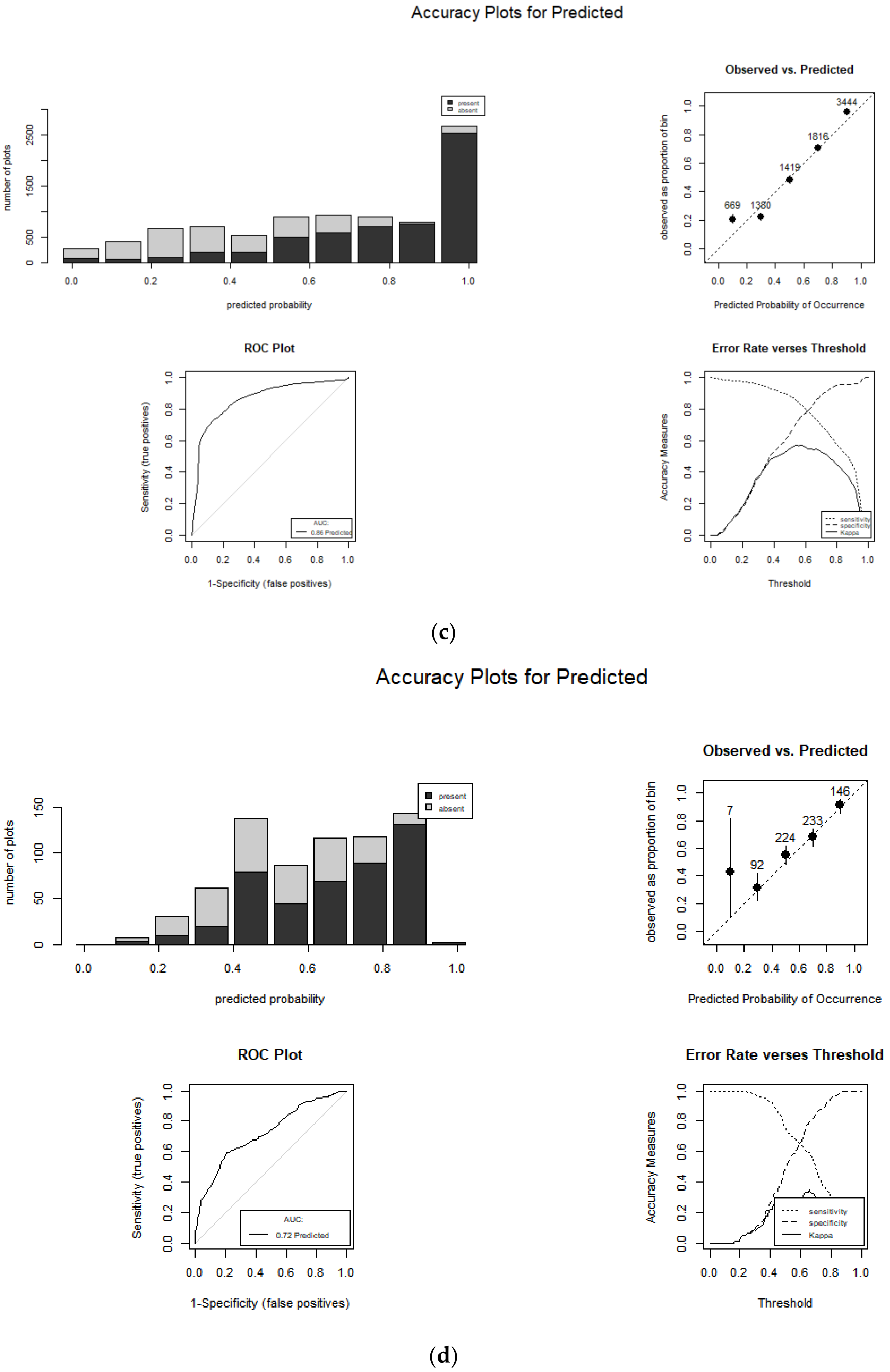
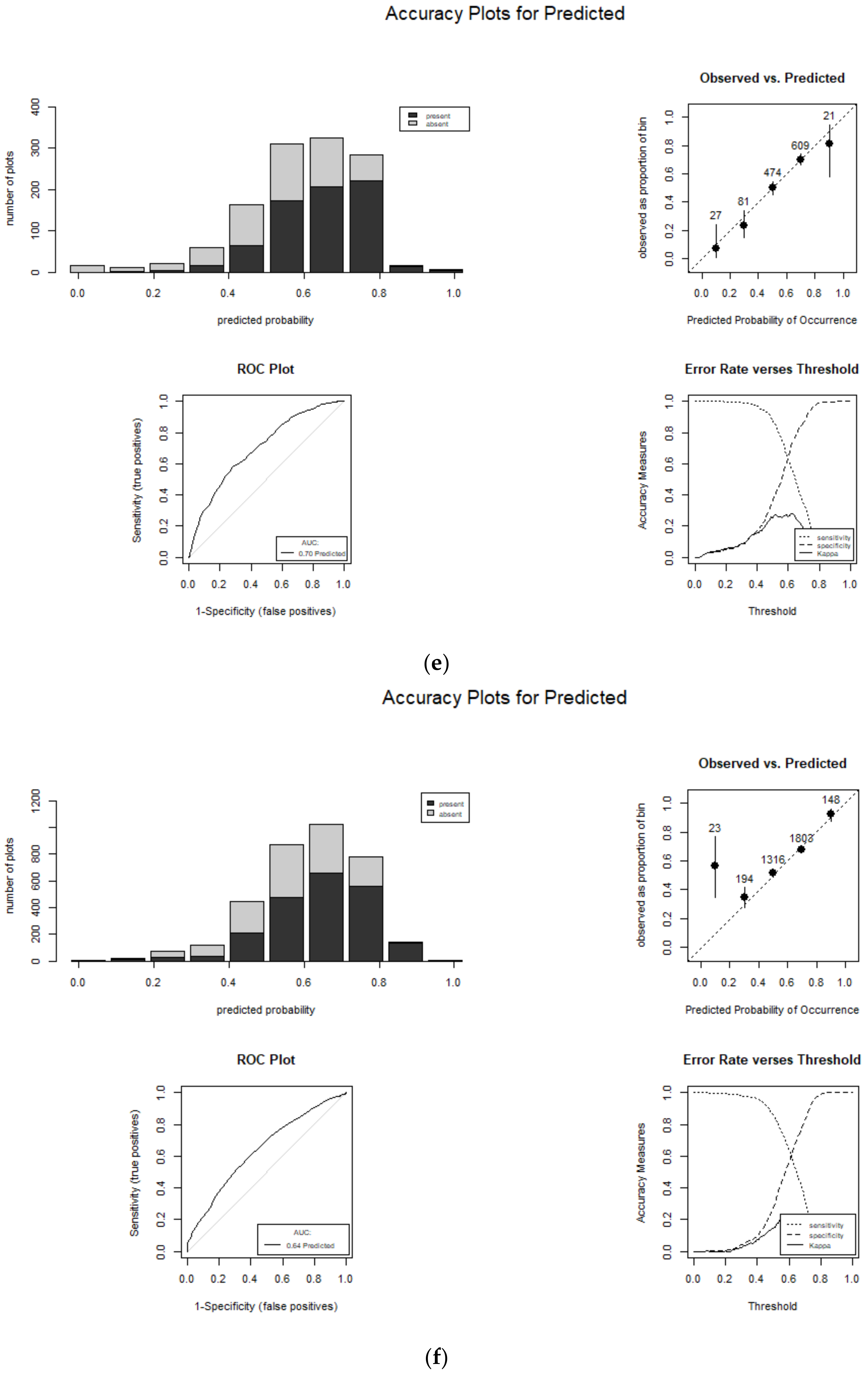
4.3. Model Validation

In all the study sites, the stepwise forward and backward BLR yielded the same model outcomes. The performances of these two models were better than the model fitted with only the intercept and the “full model” with all the predictors included. The best model selection was identified by the lowest AIC, Log Likelihood Ratio, BIC, and the residual deviance (Table 3 and Table 4). Here, we presented the results of the forward fitting model since this identifies and ranks the most important predictors from the best to the least, which was the main objective of this study (Table 3 and Table 4). As mentioned in Section 3, the ROC curve (AUC, see Figure 4 and Table 4) was used as a performance metric to assess the predictive accuracy of the BLR model. AUC values range from 0 to 1. Model fitting is best when AUC ≥ 0.7. The (AUC) of the BLR model were 0.88, 0.75, 0.88, 0.72, 0.70, and 0.64 in Diourbel-Louga-Senegal, Hodh el Gharbi-Mauritania, Zinder-Maradi-Niger, Centre-Centre Sud-Burkina Faso, Ashanti-Ghana, and Niger State-Nigeria, respectively. The model performance was better in the arid regions, i.e., Diourbel-Louga, Senegal = 0.88, Hodh el Gharbi, Mauritania = 0.75, and Zinder-Maradi, Niger = 0.88, than in the humid regions, i.e., Centre-Centre Sud, Burkina Faso = 0.72, Ashanti Region, Ghana = 0.70, and Niger State, Nigeria=0.64. Figure 5 shows the predicted probability maps and the observed LULC maps in the study sites. The BLR model fitted with only socio-economic human activities and accessibility indicators, i.e., HANPP, livestock density, population density, and travel time to urban resources, performed better than with only a wetness index, slope, elevation, and soil type in all the study sites except in Hodl el Gharbi, Mauritania. At the latter site, the model fitted with only natural predictors gave a higher AUC than with the socio-economic indicators only (Table 4).

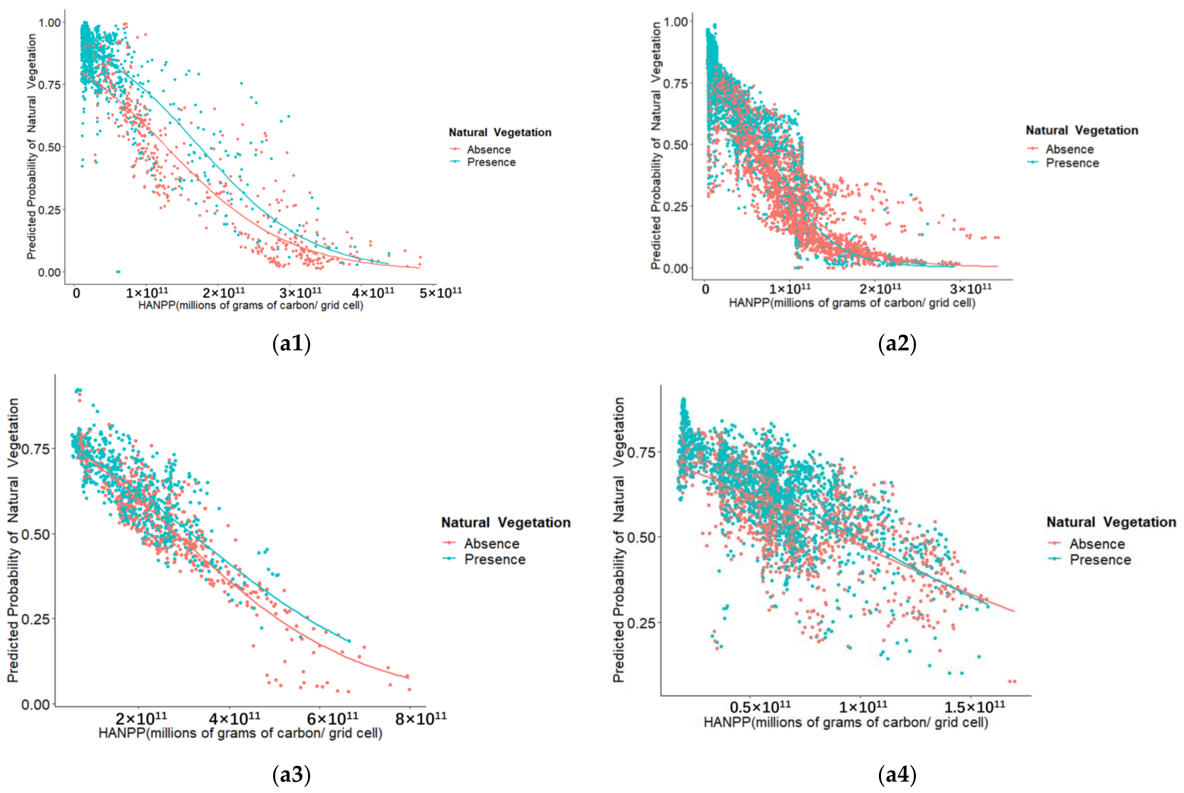
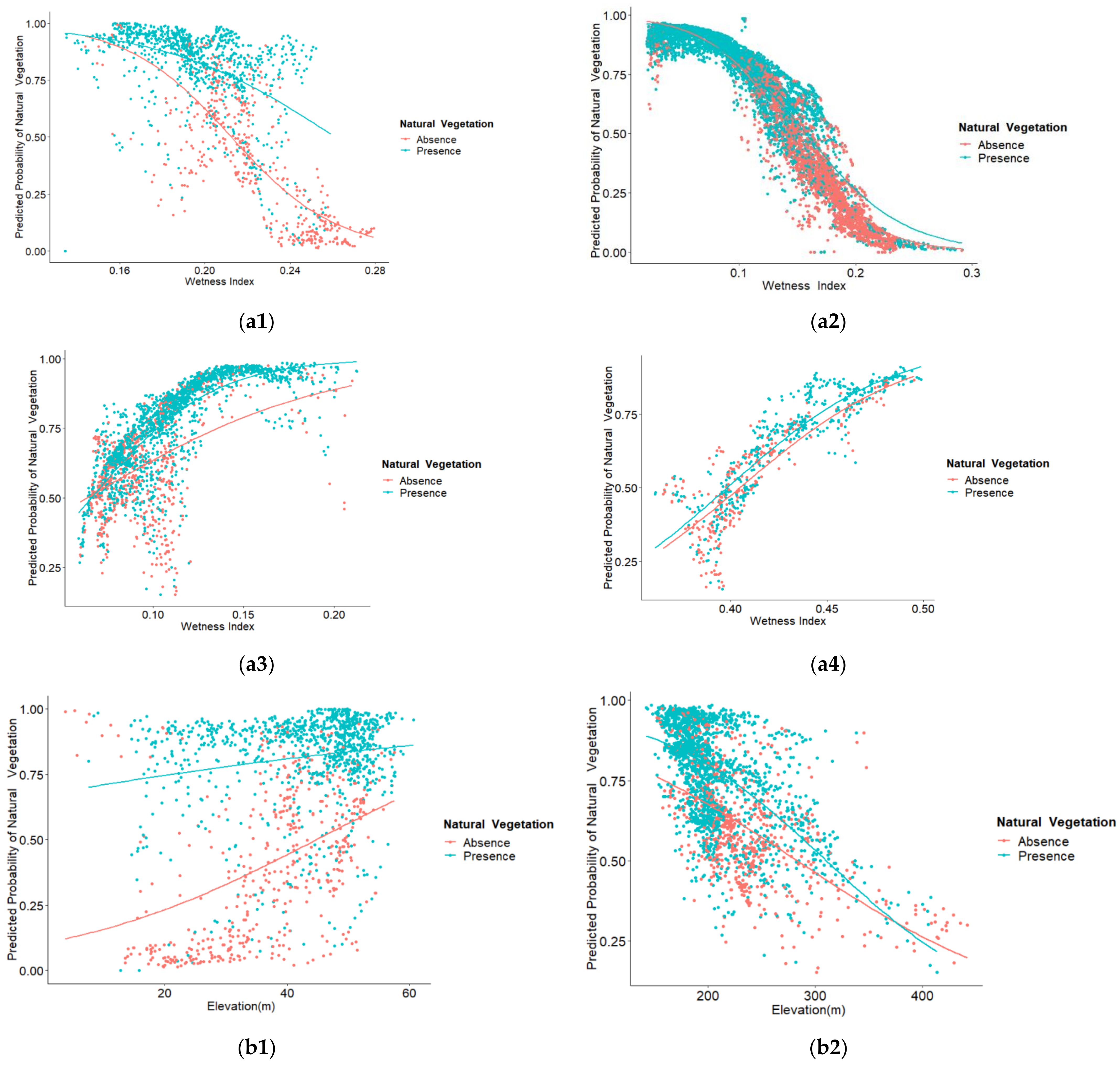
4.4. The Relationship between the Significant Underlying Drivers and Natural Vegetation

The sign of each coefficient of the predictors is a measure of the magnitude and direction of change in the probability of presence of natural vegetation in response to a change in a predictor (Table 3, Figure 6 and Figure 7). Positive coefficients of the predictors indicate that increasing the effect of the predictors will increase the likelihood of natural vegetation’s occurrence (presence) and vice versa (see Table 3 and Table 5, Figure 6(b3–b4,c1–c3) and Figure 7(a3–a4,b1)). On the contrary, negative coefficients of the predictor variables indicate that increasing the effect of the predictor variable will decrease the likelihood of natural vegetation’s occurrence (see Table 3 and Table 5, Figure 6(a1–a4,c4) and Figure 7(a1–a2,b2)). We observed a consistent negative impact of HANPP on the presence of natural vegetation across all the study sites (see Table 3 and Table 5, and Figure 6(a1–a4)). In many cases, the wetness index was insignificant in the humid regions, i.e., the Ashanti Region of Ghana and Niger State in Nigeria, characterized by intensive anthropic activities, i.e., high HANPP and livestock density (see Table 3 and Table 5). In areas where the wetness index was a significant predictor, the effect on natural vegetation was different depending on the specific conditions of the site (see Table 3 and Table 5 and Figure 7(a1–a4)).

The likelihood of natural vegetation’s occurrence was lower in the southern parts of Zinder-Maradi-Niger and Diourbel-Louga in Senegal where the wetness index and human activities (HANPP) were relatively higher compared to the northern parts of the same regions (see Table 3 for all the cases, Figure 6(a1,a2) and Figure 7(a1,a2)) for graphical representations of the cases in Diourbel-Louga, Senegal, and Zinder-Maradi, Niger, respectively. Here, the effect of wetness index on the presence of natural vegetation was negative. The reverse was true. For example, Centre-Centre Sud in Burkina Faso, i.e., in the same study site, the likelihood of natural vegetation occurrence was higher in locations, with a higher wetness index (more humid conditions), while human activities were intensive in areas with a lower wetness index. In this region (see Table 3 and Table 5 and Figure 7(a4)), the wetness index had a positive impact on the occurrence of natural vegetation in line with the natural pattern.

Population density had a negative impact on the presence of natural vegetation in all the study sites except Diourbel-Louga in Senegal, where we observed a positive impact. The impact of livestock density on natural vegetation was negative in two humid and sub-humid regions, i.e., Niger State-Nigeria and Centre-Centre Sud in Burkina Faso and one semi-arid region, i.e., the Diourbel-Louga in Senegal (see Table 3 and Table 5, Figure 6(b1,b2) for some of the cases). By contrast, the impact was positive in two arid regions, i.e., Hodh el Gharbi-Mauritania and Zinder-Maradi-Niger, and one humid region, i.e., the Ashanti Region of Ghana (see Table 3 and Table 5, Figure 6(b3,b4) for some of the cases). In the Ashanti Region, livestock density was lower in the highly urbanized areas where HANPP and population density were extremely high. In other words, HANPP and population density were negatively correlated with livestock density, but the strength of the correlation was weak to suggest multi-collinearity and the significance level of livestock density was low (see Table 3).

Accessibility measured by travel time to urban areas with population greater than 2 × 10⁴ of people had a positive impact on natural vegetation in Ashanti Region of Ghana, Niger State in Nigeria and Diourbel-Louga in Senegal (see Table 3 and Table 5, Figure 6(c1–c3)). Travel time to urban areas was an insignificant driver in Center-Center-Sud in Burkina Faso, which is a semi-humid region. On the other hand, the effect of this predictor on the presence of natural vegetation was negative in the arid regions (see Table 3 and Table 5 and Figure 6(c4)) except Diourbel-Louga in Senegal. Additionally, elevation had a negative effect on the presence of natural vegetation at all the study sites, except in Diourbel-Louga, Senegal where the impact of elevation on natural vegetation was positive (see Table 3 and Table 5, Figure 7(b1,b2)). In this area, slope and soil type had a positive impact on natural vegetation. In the other arid zones, i.e., Hodh el Gharbi-Mauritania and Zinder-Maradi-Niger, elevation, slope, and soil type had a clearly negative impact on natural vegetation (see Figure 7(b2) for the effects of elevation on the occurrence of natural vegetation at Hodh el Gharbi in Mauritania). On the contrary, slope had a positive impact on natural vegetation in Ashanti Region-Ghana and Niger State in Nigeria, while soil type impacted negatively on natural vegetation in the Ashanti Region of Ghana and positively in the Niger State of Nigeria (see Table 3 and Table 5).

5. Discussion

5.1. Multi-Collinearity

In some sites, e.g., Diourbel-Louga in Senegal, some variables exhibited collinearity (Figure 3 and Table 4). We set aside 20% of the original data for model validation and prediction. Thus, the dataset used for model predictions had the same degree of collinearity as the original dataset used to train the model. According to Harrrell Jr. [44], collinearity does not affect predictions when based on the same dataset used to estimate the model parameters, or on a new data that have the same degree of collinearity as the original data, provided extreme extrapolation is avoided. In the stepwise variable selection, collinearity can cause predictors to compete and make the selection of “important” variables arbitrary. Collinearity makes it difficult to estimate and interpret a particular regression coefficient because the predictor carries limited additional information. Despite that, we strived to eliminate redundant variables by initially identifying the potential drivers from literature. In addition, candidate predictors with a huge number of missing values were removed.

5.2. Significant Underlying Drivers Identified by the Binary Logistic Regression (BLR) Model

The BLR model provided a clear picture of which variable was significant with the corresponding p-value applying to the final predicted outcome. It revealed that the impact of the multiple sets of drivers on natural vegetation depends on other specific environmental conditions of the location under consideration, as the relationship between natural vegetation and the significant predictors varied from one study site to another for even the same predictor variables (see Table 3 and Table 5).

The stepwise variable selection technique we employed enabled us to develop a concise model with fewer predictors when possible, thereby, reducing collinearity among the multiple predictors. This prevented insignificant regression coefficients from being included in the model [44,82,83]. The major limitations of this technique have been underlined by Harrrell Jr. [44], who noted that the technique may yield a p-value, which is too small. Harrrell Jr. [44] further stressed that the problem of multi-collinearity may be compounded by applying stepwise variable selection to select randomly significant variables since the inclusion of a potential driver in the model depends on the estimated regression coefficient instead of their true values. As a result, the probability of a potential driver to be included is higher if its regression coefficient is over-estimated than the reverse [82].

According to Derksen and Keselman [83], the number of potential predictors may add noise in the model. In addition, the correlation between the predictors may affect the inclusion of genuine predictors. With respect to the dimensionality of the model, Derksen and Keselman [83] proposed that the focus of effective driver selection should be the development of an algorithm to determine beforehand the total number of potential drivers to be included, rather than focusing on the number of drivers in the final model. Harrrell Jr. [44] recommended that, prior to driver selection, multi-collinearity and driver interaction must be tested. Methods such as a full model fits or data reduction are preferable to stepwise selection algorithms. However, in the case of this study, variable selection was crucial since the major objective was to identify the important drivers based on the ranking of the predictor variables by the stepwise selection algorithm.

5.3. Model Validation

Model performance is usually assessed by evaluating whether the model can accurately predict future values of the response variables. Different model validation methods have been highlighted by Harrrell Jr. [44]. We applied data-splitting to set aside independent data for model validation. However, this approach has drawbacks since data-splitting greatly reduces the sample size for both model development and model validation. Roecker [84] noted that this method “appears to be a costly approach, both in terms of predictive accuracy of the fitted model and the precision of estimated accuracy”. Breiman [74] found that bootstrap validation on the original sample was as efficient as having a separate test sample twice as large.

In our case, the predictive accuracy of the BLR model was better in the arid regions than in the humid regions (Table 3 and Figure 4). Harrrell Jr. [44] linked poor performance of a regression model with over fitting, changes in measurement methods, changes in the definition of categorical variables, and major changes in variable inclusion criteria. The poor performance of our model in the humid ecosystem may be due to the exclusion of potentially important drivers, such as land tenure system, customs, norms, and so forth [22] in the development of the BLR model. According to Mazzucato et al. [22], the coping strategies adopted by the local informal land tenure system in Africa, have shaped the functioning of the ecosystem over years [22]. This suggests that, to obtain a perfect model fit, additional predictors must be included in the model. Among other things, a data gap in the predictor variables is one of the major limitations of this study.

5.4. The Relationship between the Significant Underlying Drivers and Occurrence of Natural Vegetation

Here, the effect of the dominant drivers, i.e., HANPP, wetness index, livestock density, and accessibility are discussed in detail from Section 5.4.1 through Section 5.4.4 with a brief discussion on the effect of soil types, slope, and elevation on the presence of natural vegetation in Section 5.4.5.

5.4.1. Human Activities (HANPP) and Demography (Population Density)

Although the relationships between the occurrence of natural vegetation and some significant drivers were location-specific, the BLR model estimated a negative relationship between HANPP and the presence of natural vegetation at all the study sites at p < 0.001. This indicates that any significant increase in HANPP will decrease the likelihood of the presence of natural vegetation (see Table 3 and Table 5 and Figure 6(a1–a4) and for the graphical representation of the cases in Diourbel Louga, Senegal, Zinder-Maradi, Niger, Ashanti Region, Ghana, and Niger State, Nigeria, respectively). This result is in agreement with Steffen et al. [4] and Ehlers and Krafft [5,85] who stated that the current human impact on the ecosystem, i.e., on natural vegetation, in particular, is pervasive at different scales. HANPP was a dominant driver in the Ashanti Region, Ghana and Diourbel-Louga in Senegal where Asenso Barnieh et al. [11] revealed a massive settlement and cropland expansions. On the other hand, vegetation recovery due to cropland abandonment was detected in some isolated areas of Diourbel-Louga by the same authors.

In-depth analysis revealed that human activities had an impact on the relationships between the presence of natural vegetation and other significant drivers, particularly the wetness index, soil type, slope, and elevation. For instance, in the Ashanti Region of Ghana, Niger State in Nigeria and Diourbel-Louga in Senegal where human activities were a dominant driver, slope had a positive impact on natural vegetation because human-induced LULC types, i.e., cropland, human settlements, and other LULC types, which were categorized as “absence of natural vegetation” in this study systematically occurred in areas with a relatively lower (gentler) slope, with the presence of natural vegetation in areas with a steeper slope (Figure 2). This signifies that crop farming and expansion of other built-up areas are avoided in areas with steeper slopes, thereby, favoring conservation of natural vegetation. Another example of how human influence may alter the response of natural vegetation to climate is the negative relationship between the occurrence of natural vegetation and the wetness index in Zinder-Maradi, Niger and Diourbel-Louga, Senegal (see Figure 7(a1,a2)). In this case, detailed analysis revealed lower probability of natural vegetation’s occurrences in locations with a higher wetness index against the natural pattern of more likely occurrence of natural vegetation with higher humidity (see Figure 2). This is consistent with the previous studies by Turner et al. [1] and Foley et al. [2] who suggested that intensive human activities at the local scale and the rapid changes in the LULC system at different scales may intensify changes in land surface climate and exacerbate the vulnerability of ecosystem services, biodiversity, water balance, and soil conditions.

Furthermore, we found that population density was directly proportional to HANPP in all the study sites except Diourbel-Louga in Senegal (see Table 3 and Table 5). In this area, there was a positive relationship between population density and the presence of natural vegetation, i.e., an increase in population density increased the likelihood of the presence of natural vegetation. Though the population density observed in this area in 2000 was comparatively high, i.e., third highest in the selected hotspots in West Africa (see Table 2), the abandonment of cropland, the subsequent replacement by natural vegetation, and migration of the farmers to bigger cities in the same study site explained the observed positive impact of population density on natural vegetation in this region [11,61,63]. Detailed validation with the geospatial raster maps used to develop the model showed denser population coupled with intensive human activities in the Diourbel Region. Here, the likelihood of natural vegetation occurrence was lower. However, toward the Louga Region, which is the greater proportion of the site, sparser population correlated with higher likelihood of natural vegetation (see Figure 2).

The negative relationship between population density and presence of natural vegetation observed in all the other sites highlights the negative impact of human activities on natural vegetation. Brandt et al. [21] underlined the “negative-population-vegetation” response in West Africa. Under this scenario, a further increase in population will exacerbate the impact of human activities on natural vegetation with serious implications for climate impact mitigation. The loss of biomass and carbon through deforestation and degradation of natural resources increases the emission of greenhouse gases into the atmosphere. In densely populated regions, e.g., Ashanti Region in Ghana, Niger State in Nigeria and Diourbel-Louga in Senegal, the significance (see Table 3 and Table 5) of population density, in explaining the presence of natural vegetation was lower since population densities in these regions were localized in few major cities (see Table 2 for the descriptive statistics and Figure 2 for spatial distribution). This finding is consistent with the LULC transitions mapping by Asenso Barnieh et al. [11] who found that human settlement expansions in West Africa are localized in only a few areas.

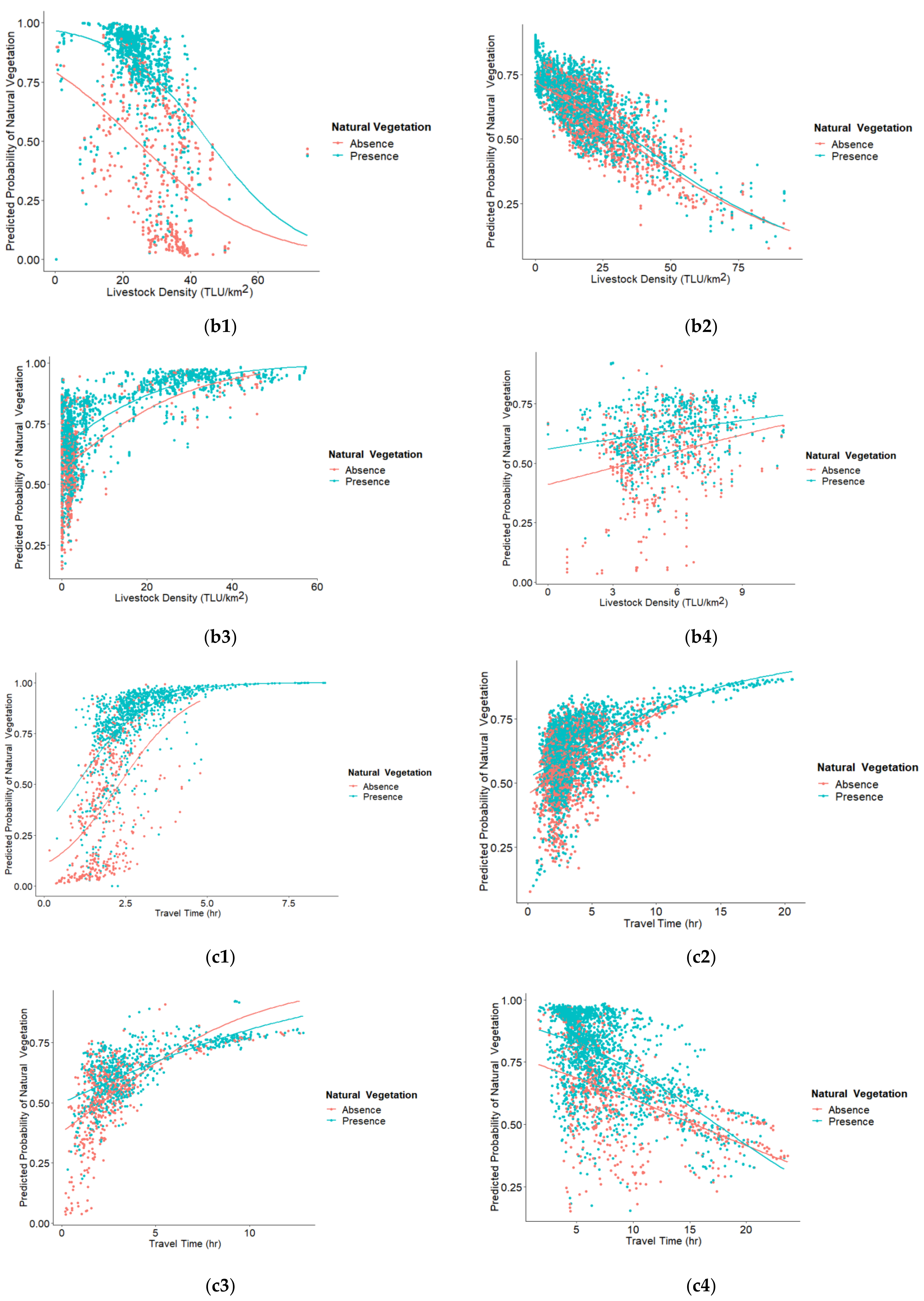
5.4.2. Livestock Density

In the sites in Diourbel-Louga, Senegal, Centre-Centre Sud in Burkina Faso, and Niger State in Nigeria, with very high livestock density (see Table 2), the BLR model predicted a negative impact of livestock density, especially cattle, on the presence of natural vegetation (see Table 3 and Table 5 and Figure 6(b1,b2) for graphical representations of the cases in Diourbel-Louga, Senegal and Niger State, Nigeria). In reality, grazing and trampling pressure by livestock have negative impacts on total above ground biomass with pressure, increasing when livestock density increases [58,86,87,88]. This is consistent with the findings from this study. Furthermore, in the previously mentioned areas, nomadism and transhumance are well practiced. Mobility of herds through nomadism (i.e., herds migrate over long distances from season to season in search of pasture) and transhumance are well-known coping strategies by livestock keepers in West Africa for ensuring the survival of livestock when the availability of natural vegetation is low during the dry season. This system of livestock management has a greater impact on natural vegetation when the movement of the animals are unguided [58,87,89,90]. Here, the proportion of livestock occurrence in the highly urbanized area was higher than in the less urbanized area where the fractional abundance of natural vegetation was higher (see Figure 2). Therefore, apart from the negative impact of livestock density on the presence of natural vegetation, other human activities tied with urbanization may play a role in the displacement of natural vegetation in these sites.

According to Schlecht et al. [88], in highly populated and urbanized areas, livestock farmers dispose livestock dung in open spaces and streets. The exposure of dung to extreme sunlight and rainfall has negative implications on the environment since the process may lead to leaching of nutrients and emission of greenhouse gases, such as methane to the atmosphere with a subsequent impact on climate. In Burkina Faso, roadside grasses, fallowed vegetation and stubble material from public spaces within and particularly around the city, are contributing a significant share of dry matter intake of ruminants in Ouagadougou, which is one of the urbanized areas in the study site in Centre-Centre Sud of Burkina Faso [88].

On the contrary, in the study sites in Hodh el Gharbi, Mauritania, Ashanti Region, Ghana, and Zinder-Maradi, Niger where positive relationships (see Table 3 and Table 5, Figure 2 and Figure 6(b3,b4) for the cases in Hodh el Gharbi, Mauritania and Ashanti Region, Ghana) were predicted between the presence of natural vegetation and livestock density by the BLR model. The livestock densities were relatively lower (Table 2) and the types of livestock were restricted to small ruminants, such as goat and sheep with restricted livestock movement [90]. Though Mauritania is well known for its dependence on nomadic and transhumance livestock farming, the site in Hodh el Gharbi had a relatively lower livestock density (see Table 2 and Figure 2) with restricted livestock movement and impact on natural vegetation compared with other parts of the country [90].

Livestock rearing in the Ashanti Region of Ghana is not nomadic. Livestock farmers mostly depend on a wide variety of feed resources such as grass and peels of cassava, plantain, and agro-industrial by-products like millet mash residue, rice bran, and home waste to feed their cattle [91]. This reduces the grazing pressure by livestock. Moreover, livestock density is more likely to have a positive impact on the presence of natural vegetation in areas where livestock are used as manpower for crop cultivation, e.g., Hodh el Gharbi, and where crop residues are used to feed the livestock. Such symbiotic association between livestock rearing and crop farming, as in some rural and peri-urban areas in the Ashanti Region, Ghana and Zinder Maradi, Niger is more likely to lead to a positive impact of livestock density on the presence of natural vegetation (Table 3 and Table 5 and Figure 2) as predicted by the BLR model since crop residues augment herbaceous vegetation for grazing, thereby, easing the pressure on natural vegetation cover [89].

5.4.3. Accessibility (Travel Time)

The negative or positive (see Table 3 and Table 5 and Figure 6(c1–c4)) influence of accessibility on the presence of natural vegetation may be related to the differences in the type and spatial distribution of natural vegetation as well human settlements.

In the humid and highly urbanized regions, i.e., Ashanti Region in Ghana and Niger State in Nigeria, where wetness was not a limiting factor, the BLR model predicted a positive relationship between travel time to urban resources and the presence of natural vegetation (see Table 3 and Table 5 and Figure 6(c2,c3)). In these sites, the rate of natural vegetation conversion to human settlement, cropland, and other industrial developments between 1975 and 2000 was unprecedented [11]. The only types of natural vegetation spared from land conversion in these areas were protected forest and natural vegetation in the rural areas. The closer the cities to land area allocated for natural vegetation conservation and protection, the higher the rate of conversions and, hence, as travel time increases, the likelihood of the presence of natural vegetation increases (see Figure 2). Therefore, natural protected areas in such areas may be sited very far away from urban areas. Diourbel-Louga in Senegal is an arid region with spatial patterns similar to the previously mentioned areas in the humid region (see Figure 6(c1)). Here, the model predicted a positive impact of travel time on natural vegetation.

The reverse was true for the study sites in Zinder-Maradi in Niger and Hodh el Gharbi in Mauritania where wetness was a limiting factor and human settlements were in close proximity with natural vegetation and better climate conditions. In this case, a negative relationship between travel time and natural vegetation was estimated by the BLR model (see Table 2, Table 3 and Table 5 and Figure 6(c4) for the case in Hodh el Gharbi, Mauritania). However, HANPP in the relatively more humid and urbanized areas was high. In the Zinder-Maradi Region, for example, farmers have adopted management practices. The areas very far from the cities were degraded due to the repeated episodes of severe drought in the 1970s and 1980s [64,65]. Under these conditions, increasing travel time to urban resources decreases the likelihood of the presence of natural vegetation (Figure 2). This is in agreement with the analysis of distribution and trend in vegetation in some sections of the Zinder-Maradi site by Rishmawi and Prince [27], who highlighted that areas far from human settlements were prone to a biomass productivity decline. Leroux et al. [28] found that increasing travel time had a negative impact on biomass productivity in some parts of the study area. Therefore, natural protected areas in such Regions must be cited in close proximity to human settlements under strict management and protection. The Sahel Great Green Belt Initiative is a call in the right direction [92,93].

5.4.4. Climate (Wetness Index)

The predictions from the BLR model suggested that the wetness index was neither the only underlying driver nor the dominant driver of the presence of natural vegetation in West Africa prior to the period of 2000. The wetness index was insignificant at p < 0.05 in some study sites, particularly in the humid regions, e.g., the Ashanti Region-Ghana and Niger State-Nigeria (see Table 3 and Table 5). This contradicts previous studies by Anyamba and Tucker [19], Hickler et al. [17], Seaquist et al. [18], and Huber et al. [20], who noted that climate variability is the major underlying driver of vegetation dynamics in Africa, particularly in the Sahel region. In Diourbel-Louga in Senegal, which falls within the Sahel (arid) region, the step-wise forward BLR model revealed that human activity as measured by HANPP was the dominant driver of the presence of natural vegetation (see Table 3 and Table 5). The relationship determined by the BLR model is supported by the previous LULC transitions analyses of Asenso Barnieh et al. [11], who revealed a massive settlement and cropland expansion with isolated cropland decline due to abandonment in Senegal.

Even in the study sites where the wetness index was the leading underlying driver, the sub-models demonstrated that the model with human socio-economic activities predictors only explained a greater proportion of variability in the presence of natural vegetation than the natural predictors’ only (see Table 3). In addition, the impact of the wetness index on natural vegetation was different and controlled by human activities across the sub-continent, as described earlier (see Table 3 and Figure 7(a1–a4)). With limited human activities, a higher wetness index will increase the presence of natural vegetation, as in the case of Hodh el Gharbi in Mauritania (Figure 2 and Figure 7(a3,a4).

Despite the fact that the impact of wetness index on natural vegetation was positive in both Hodh el Gharbi in Mauritania and Centre-Centre Sud in Burkina Faso (see Table 3 and Table 5, Figure 7(a3,a4)), we observed that the impact in Hodh el Gharbi in Mauritania was random while the impact in Centre-Centre-Sud in Burkina Faso was systematic. This is because we found a direct relationship between population density, HANPP, and livestock density, and the wetness index in Hodh el Gharbi-Mauritania (Figure 3b). Nonetheless, toward the northern part of the study site, there was a vast area of degraded land. Visual analysis of the HANPP and livestock density geospatial data (Figure 2) revealed little human impact and a clearer impact of climate, such as repeated episodes of drought in this area. Comparatively, human socio-economic activities measured by population density, livestock density, and HANPP were relatively lower at this study site (Table 2). The sub-model fitted with only natural predictors explained a greater proportion of the variability in the occurrence of natural vegetation than the sub-model fitted with only human socio-economic predictors in this study site. This is consistent with the LULC transition analysis by Asenso Barnieh et al. [11] who revealed massive natural vegetation replacement by sandy dunes and bare land linked with climate in this region. Hoscilo et al. [94] found a positive relationship between rainfall and normalized difference vegetation index NDVI, which is a proxy for biomass productivity in Mauritania.

On the contrary, an inverse relationship was found between population density, HANPP, and livestock density and the wetness index in Centre-Centre Sud in Burkina Faso (Figure 3d). Here, socio-economic indices were relatively high (see Figure 2) in the far arid north. Generally, human socio-economic indicators in this study site were higher in comparison with other study sites apart from the Ashanti Region of Ghana (see Table 2). The wetness index was higher in the areas toward the humid south, far from human settlements with little human activities whose impact is coupled with very dense natural vegetation. These areas were spared from land conversion between 1975–2000 [11] (see Figure 2 for spatial distribution of natural vegetation). The natural vegetation distribution here followed the natural pattern suggesting that, in spite of human socio-economic growth, systematic spatial planning may sustain the positive response of natural vegetation to precipitation and mitigate its sensitivity to disturbances (see Figure 7(a4)).

In Diourbel-Louga of Senegal and Zinder-Maradi in Niger, where the impact of the wetness index on natural vegetation was negative, the effect of the wetness index on natural vegetation was controlled by the intensity of human activities, i.e., a positive relationship was found between HANPP, livestock density, population density, and the wetness index (see Figure 2 and Figure 3a,c), with the presence of natural vegetation decreasing while increasing the wetness index (see Figure 7(a1,a2) for a graphical representation of the case in Diourbel-Louga and Zinder-Maradi). In these two areas, previous studies have documented massive expansions of croplands at the more humid southern parts where the wetness index is higher and natural vegetation has been replanted at the water deficit areas under the “farmer-managed natural resources’ regeneration initiative” [64,65].

5.4.5. Soil Type, Elevation, and Slope

The BLR model predicted (see Table 3 and Table 5 and Figure 2) a positive effect of soil type on the presence of natural vegetation in Centre-Centre Sud of Burkina Faso, Niger State of Nigeria, and Diourbel-Louga of Senegal, where the dominant soil types, i.e., Nitisols, Luvisols, Fluvisols, Arenosols, and Cambisols, are fertile and a negative effect in the Ashanti Region of Ghana, Hodh el Gharbi of Mauritania, and Zinder-Maradi of Niger, where the dominant soil types, i.e., Acrisol, Lithisols, and Regosols, are sub-optimal for natural vegetation growth [55]. With regard to the effect of slope and elevation on occurrence of natural vegetation, naturally, gentle slopes and lower elevations are generally more suitable for vegetation growth [54]. This is consistent with the negative effects of elevation on natural vegetation, i.e., increasing elevation decreased the odds of the occurrence of natural vegetation, estimated by the BLR model at all the study sites (see Table 3 and Figure 7(b2) for a graphical representation of the case in Hodh el Gharbi, Mauritania), except in Diourbel-Louga in Senegal (see Figure 7(b1)) where a higher elevation increased the presence of natural vegetation.

Slope controls soil water content by influencing infiltration, drainage, and runoff [95,96,97,98] and it is a determinant of soil erosion and degradation, with an impact on vegetation growth [99]. In the Ashanti Region of Ghana, Diourbel-Louga of Senegal, and Niger State of Nigeria, human activities were influential drivers (see Table 3 and Table 5) and slope had a positive impact on natural vegetation, i.e., steeper slopes increased the odds of natural vegetation occurrence because humans induced LULC types, i.e., cropland and human settlements systematically occur in areas with a gentler slope (see Table 3 and Table 5 and Figure 2). The results of this study provide enough evidence to support the conclusion that “a single factor explanation of a LULC change in Africa”, i.e., of the occurrence of natural vegetation is not enough [14]. Our findings are in agreement with the findings of Boschetti et al. [25] and Leroux et al. [28] who stated that the LULC change in West Africa is determined by interplay of climate, biophysical, and anthropogenic drivers.

6. Conclusions

This research demonstrated the ability of the BLR model to identify statistically significant drivers, which determine the presence of natural vegetation in a complex ecosystem where a single driver explanation was not sufficient. The BLR model revealed not only the statistically significant multiple set of underlying drivers of natural vegetation’s occurrence, but also the interplay of these drivers and their relative impacts. The study revealed that, even prior to 2000, human activities as measured by HANPP were pervasive and a significant driver of natural vegetation in West Africa. The likelihood of natural vegetation’s occurrence decreases with increasing human activities in all the study sites. Moreover, the relationships between the presence of natural vegetation and all the other drivers were location-specific and mostly depended on the intensity of human activities. The study highlights the significant role human activities play in altering the land surface climate and natural indicators as well as the ecosystem. Thus, without a negative human influence, the relationship between natural vegetation and natural drivers, i.e., wetness index, slope, elevation, and soil type, leads to positive effects on the ecosystem, but intensive human activities may trigger negative changes in the ecosystem. Therefore, development of policies and strategies to control the intensity of human activities and to revamp the degraded landscape are urgently needed in West Africa. The results from this study may provide useful information for understanding the interactions between human and the environment for natural resources management, climate change adaptation, and sustainable development. The past responses of natural vegetation to multiple underlying drivers captured by this research may serve as a foundation to predict the current occurrences of natural vegetation and projections into the future. The BLR model approach is advancement over the traditional narrations and people’s perceptions on underlying drivers of natural vegetation’s dynamics in West Africa.

References

1. Turner, A.B.L.; Meyer, W.B.; Skole, D.L. Global Land-Use/Land-Change: Towards an Integrated Study. Integr. Earth Syst. Sci. 2009, 23, 91–95. [Google Scholar]
2. Foley, J.A.; Defries, R.; Asner, G.P.; Barford, C.; Bonan, G.; Carpenter, S.R.; Chapin, F.S.; Coe, M.T.; Daily, G.C.; Gibbs, H.K.; et al. Global Consequences of Land Use. Science 2010, 309, 570–574. [Google Scholar] [CrossRef] [Green Version]
3. Lambin, E.F.; Geist, H.J.; Lepers, E. Dynamics of land-use and land-cover change in tropical regions. Annu. Rev. Environ. Resour. 2003, 28, 206–216. [Google Scholar] [CrossRef] [Green Version]
4. Steffen, W.; Sanderson, A.; Tyson, P.; Jäger, J.; Matson, P.; Moore, B., III; Oldfield, F.; Oldfield, F.; Richardson, K.; Oldfield, F.; et al. Global Change and the Earth System: A Plane under Pressure; Springer: Berlin/Heidelberg, Germany, 2005; ISBN 9783540265948. [Google Scholar]
5. Ehlers, E.; Krafft, T. (Eds.) Earth System Science in the Anthropocene; Springer: Berlin/Heidelberg, Germany, 2016; Volume 53, ISBN 9788578110796. [Google Scholar]
6. UNEP. Sahel Atlas of Changing Landscapes:Tracing Trends and Variations in Vegetation Cover and Soil Condition; UNEP: Nairobi, Kenya, 2012; ISBN 9789280733006. [Google Scholar]
7. Nicholson, S.E.; Tucker, C.J.; Ba, M.B. Desertification, drought, and surface vegetation: An example from the West African sahel. Bull. Am. Meteorol. Soc. 1998, 79, 815–830. [Google Scholar] [CrossRef]
8. Hulme, M. Climatic perspectives on Sahelian desiccation: 1973 1998. Glob. Environ. Chang. 2001, 11, 19–29. [Google Scholar] [CrossRef] [Green Version]
9. Tucker, C.J.; Dregne, H.E.; Newcomb, W.W. Expansion and contraction of the Sahara Desert from 1980 to 1990. Science 1991, 253, 299–301. [Google Scholar] [CrossRef]
10. Nicholson, S.E. Land surface-atmosphere interaction: Physical processes and surface changes and their impact. Prog. Phys. Geogr. 1988, 12, 36–65. [Google Scholar] [CrossRef]
11. Asenso Barnieh, B.; Jia, L.; Menenti, M.; Zhou, J.; Zeng, Y. Mapping Land Use Land Cover Transitions at Different Spatiotemporal Scales in West Africa. Sustainability 2020, 12, 8565. [Google Scholar] [CrossRef]
12. Brink, A.B.; Eva, H.D. Monitoring 25 years of land cover change dynamics in Africa: A sample based remote sensing approach. Appl. Geogr. 2009, 29, 501–512. [Google Scholar] [CrossRef]
13. Vittek, M.; Brink, A.; Donnay, F.; Simonetti, D.; Desclé, B. Land Cover Change Monitoring Using Landsat MSS/TM Satellite Image Data over West Africa between 1975 and 1990. Remote Sens. 2014, 6, 658–676. [Google Scholar] [CrossRef] [Green Version]
14. Lambin, E.F.; Turner, B.L.; Geist, H.J.; Agbola, S.B.; Angelsen, A.; Folke, C.; Bruce, J.W.; Coomes, O.T.; Dirzo, R.; George, P.S.; et al. The causes of land-use and land-cover change: Moving beyond the myths. Glob. Environ. Chang. 2001, 11, 261–269. [Google Scholar] [CrossRef]
15. Geist, H.J.; Lambin, E.F. Proximate Causes and Underlying Driving Forces of Tropical Deforestation. Bioscience 2002, 52, 143–150. [Google Scholar] [CrossRef]
16. Chomitz, K.M.; Gray, D.A. Roads, Land Use, and Deforestation: A Spatial Model Applied to Belize Roads, Land Use, and Deforestation. World Bank Econ. Rev. 1996, 10, 487–512. [Google Scholar] [CrossRef] [Green Version]
17. Hickler, T.; Eklundh, L.; Seaquist, J.W.; Smith, B.; Ardo, J.; Olsson, L.; Sykes, M.T.; Sjo, M. Precipitation controls Sahel greening trend. Geophys. Res. Lett. 2005, 32, 2–5. [Google Scholar] [CrossRef]
18. Seaquist, J.W.; Hickler, T.; Eklundh, L.; Ardö, J.; Heumann, B.W. Disentangling the effects of climate and people on Sahel vegetation dynamics. Biogeosciences 2009, 6, 469–477. [Google Scholar] [CrossRef]
19. Anyamba, A.; Tucker, C.J. Analysis of Sahelian vegetation dynamics using NOAA-AVHRR NDVI data from 1981 – 2003. J. Arid Environ. 2005, 63, 596–614. [Google Scholar] [CrossRef]
20. Huber, S.; Fensholt, R.; Rasmussen, K. Water availability as the driver of vegetation dynamics in the African Sahel from 1982 to 2007. Glob. Planet. Change 2011, 76, 186–195. [Google Scholar] [CrossRef]
21. Brandt, M.; Rasmussen, K.; Peñuelas, J.; Tian, F.; Schurgers, G.; Verger, A.; Mertz, O.; Palmer, J.R.B.; Fensholt, R. Human population growth offsets climate-driven increase in woody vegetation in sub-Saharan Africa2. Nat. Ecol. Evol. 2017, 1, 4–9. [Google Scholar] [CrossRef] [PubMed] [Green Version]
22. Mazzucato, V.; Niemeijer, D.; Mazzucato, V.; Niemeijer, D. Population Growth and the Environment in Africa: Local Informal Institutions, the Missing Link. Econ. Geogr. 2009, 78, 171–193. [Google Scholar] [CrossRef]
23. Herrmann, S.M.; Brandt, M.; Rasmussen, K.; Fensholt, R. Accelerating land cover change in West Africa over four decades as population pressure increased. Commun. Earth Environ. 2020, 1. [Google Scholar] [CrossRef]
24. Linard, C.; Gilbert, M.; Snow, R.W.; Noor, A.M.; Tatem, A.J. Population Distribution, Settlement Patterns and Accessibility across Africa in 2010. PLoS One 2012, 7. [Google Scholar] [CrossRef] [PubMed] [Green Version]
25. Boschetti, M.; Nutini, F.; Brivio, P.A.; Bartholomé, E.; Stroppiana, D.; Hoscilo, A. Identification of environmental anomaly hot spots in West Africa from time series of NDVI and rainfall. ISPRS J. Photogramm. Remote Sens. 2013, 78, 26–40. [Google Scholar] [CrossRef]
26. Brandt, M.; Hiernaux, P.; Rasmussen, K.; Mbow, C.; Kergoat, L.; Tagesson, T.; Ibrahim, Y.Z.; Wélé, A.; Tucker, C.J.; Fensholt, R. Assessing woody vegetation trends in Sahelian drylands using MODIS based seasonal metrics. Remote Sens. Environ. 2016, 183, 215–225. [Google Scholar] [CrossRef] [Green Version]
27. Rishmawi, K.; Prince, S.D. Environmental and anthropogenic degradation of vegetation in the Sahel from 1982 to 2006. Remote Sens. 2016, 8, 948. [Google Scholar] [CrossRef] [Green Version]
28. Leroux, L.; Bégué, A.; Lo, D.; Jolivot, A.; Kayitakire, F. Driving forces of recent vegetation changes in the Sahel: Lessons learned from regional and local level analyses. Remote Sens. Environ. 2017, 191, 38–54. [Google Scholar] [CrossRef] [Green Version]
29. Kleemann, J.; Baysal, G.; Bulley, H.N.N.; Fürst, C. Assessing driving forces of land use and land cover change by a mixed-method approach in north-eastern Ghana, West Africa. J. Environ. Manage. 2017, 196, 411–442. [Google Scholar] [CrossRef]
30. Verburg, P.H.; van Eck, J.R.R.; de Nijs, T.C.M.; Dijst, M.; Schot, P. Determinants of land-use change patterns in the Netherlands. Environ. Plan. B Plan. Des. 2004, 31, 125–150. [Google Scholar] [CrossRef] [Green Version]
31. Fasika, A.; Motuma, T.; Gizaw, T. Land Use Land Cover Change Trend and Its Drivers in Somodo Watershed South Western, Ethiopia. African J. Agric. Res. 2019, 14, 102–117. [Google Scholar] [CrossRef] [Green Version]
32. Betru, T.; Tolera, M.; Sahle, K.; Kassa, H. Trends and drivers of land use / land cover change in Western Ethiopia. Appl. Geogr. 2019, 104, 83–93. [Google Scholar] [CrossRef]
33. Pricope, N.G.; Husak, G.; Lopez-carr, D. The climate-population nexus in the East African Horn: Emerging degradation trends in rangeland and pastoral livelihood zones Narcisa. Glob. Environ. Chang. 2013, 23, 1525–1541. [Google Scholar] [CrossRef]
34. Braimoh, A.K.; Vlek, P.L.G. Scale-Dependent Relationships between Land-Use Change and Its Determinants in the Volta Basin of Ghana. Earth Interact. 2004, 8, 1–23. [Google Scholar] [CrossRef]
35. Kindu, M.; Schneider, T.; Döllerer, M.; Teketay, D.; Knoke, T. Scenario modelling of land use / land cover changes in Munessa-Shashemene landscape of the Ethiopian highlands. Sci. Total Environ. 2018, 623, 534–546. [Google Scholar] [CrossRef]
36. Nelder, J.; Wedderburn, R.W.M. Generalized linear models. J. R. Stat. Soc. 1972, A135, 370–384. [Google Scholar] [CrossRef]
37. McCullough, P.; Nelder, J.A. Generalized Linear Models, 2nd ed.; Chapman & Hall: New York, NY, USA, 1989. [Google Scholar]
38. Ayalew, L.; Yamagishi, H. The application of GIS-based logistic regression for landslide susceptibility mapping in the Kakuda-Yahiko Mountains, Central Japan. Geomorphology 2005, 65, 15–31. [Google Scholar] [CrossRef]
39. Razanamahandry, L.C.; Andrianisa, H.A.; Karoui, H.; Podgorski, J.; Yacouba, H. Prediction model for cyanide soil pollution in artisanal gold mining area by using logistic regression. Catena 2018, 162, 40–50. [Google Scholar] [CrossRef]
40. Shu, B.; Zhang, H.; Li, Y.; Qu, Y.; Chen, L. Spatiotemporal variation analysis of driving forces of urban land spatial expansion using logistic regression: A case study of port towns in Taicang City, China. Habitat Int. 2014, 43, 181–190. [Google Scholar] [CrossRef]
41. Hemasinghe, H.; Rangali, R.S.S.; Deshapriya, N.L.; Samarakoon, L. Landslide susceptibility mapping using logistic regression model (a case study in Badulla District, Sri Lanka). Proc. Eng. 2018, 212, 1046–1053. [Google Scholar] [CrossRef]
42. Fox, J.; Weisberg, S. An R Companion to Applied Regression, 3rd ed.; SAGE Publications: Los Angeles, CA, USA, 2018; ISBN 9781544336459. [Google Scholar]
43. Yalcin, A.; Reis, S.; Aydinoglu, A.C.; Yomralioglu, T. A GIS-based comparative study of frequency ratio, analytical hierarchy process, bivariate statistics and logistics regression methods for landslide susceptibility mapping in Trabzon, NE Turkey. Catena 2011, 85, 274–287. [Google Scholar] [CrossRef]
44. Harrrell, F.E., Jr. Regression Modeling Strategies, 2nd ed.; Springer: Nashville, TN, USA, 2015; Volume 45, ISBN 9783319194240. [Google Scholar]
45. Mazzocco, T.; Hussain, A. Novel logistic regression models to aid the diagnosis of dementia. Expert Syst. Appl. 2012, 39, 3356–3361. [Google Scholar] [CrossRef]
46. Cao, Y.; Zhang, X.; Fu, Y.; Lu, Z.; Shen, X. Urban spatial growth modeling using logistic regression and cellular automata: A case study of Hangzhou. Ecol. Indic. 2020, 113, 106200. [Google Scholar] [CrossRef]
47. Menard, S. Logistic Regression: From Introductory to Advanced Concepts and Applications; SAGE Publications Inc.: Thousand Oaks, CA, USA, 2009; ISBN 9781412974837. [Google Scholar]
48. Lopez, S. Modeling Agricultural Change through Logistic Regression and Cellular Automata: A Case Study on Shifting Cultivation. J. Geogr. Inf. Syst. 2014, 06, 220–235. [Google Scholar] [CrossRef] [Green Version]
49. Das, I.; Sahoo, S.; van Westen, C.; Stein, A.; Hack, R. Landslide susceptibility assessment using logistic regression and its comparison with a rock mass classification system along a road section in the northern Himalayas (India). Geomorphology 2010, 114, 627–637. [Google Scholar] [CrossRef]
50. Tsangaratos, P.; Ilia, I. Comparison of a logistic regression and Naïve Bayes classifier in landslide susceptibility assessments: The influence of models complexity and training dataset size. Catena 2016, 145, 164–179. [Google Scholar] [CrossRef]
51. Hosmer, D.W.; Lemeshow, S. Applied Logistic Regression; John Wiley & Sons Inc.: New York, NY, USA, 2000. [Google Scholar]
52. Fitzmaurice, G.M.; Laird, N.M. Binary Response Models and Logistic Regression, 2nd ed.; Elsevier: Boston, MA, USA, 2015; Volume 2, ISBN 9780080970875. [Google Scholar]
53. Agresti, A. An Introduction to Categorical Data Analysis; Wiley: New York, NY, USA, 1996. [Google Scholar]
54. Teferi, E.; Bewket, W.; Uhlenbrook, S.; Wenninger, J. Understanding recent land use and land cover dynamics in the source region of the Upper Blue Nile, Ethiopia: Spatially explicit statistical modeling of systematic transitions. Agric. Ecosyst. Environ. 2013, 165, 98–117. [Google Scholar] [CrossRef]
55. FAO. World Reference Base for Soil Resources 2014. International Soil Classification System for Naming Soils and Creating Legends for Soil Maps; FAO: Rome, Italy, 2015; ISBN 9789251083697. [Google Scholar]
56. Trabucco, A.; Zomer, R.J. Global Aridity Index (Global-Aridity) and Global Potential Evapo-Transpiration (Global-PET) Geospatial Database. Available online: http://www.csi.cgiar.org (accessed on 22 June 2018).
57. Imhoff, M.L.; Bounoua, L.; Ricketts, T.; Loucks, C.; Harriss, R.; Lawrence, W. Global patterns in human consumption of net primary production. Nature 2004, 429, 870–873. [Google Scholar] [CrossRef] [PubMed] [Green Version]
58. Robinson, T.P.; William Wint, G.R.; Conchedda, G.; Van Boeckel, T.P.; Ercoli, V.; Palamara, E.; Cinardi, G.; D’Aietti, L.; Hay, S.I.; Gilbert, M. Mapping the global distribution of livestock. PLoS ONE 2014, 9. [Google Scholar] [CrossRef] [PubMed] [Green Version]
59. Nelson, A.; Weiss, D.J.; van Etten, J.; Cattaneo, A.; McMenomy, T.S.; Koo, J. A suite of global accessibility indicators. Sci. Data 2019, 266. [Google Scholar] [CrossRef] [Green Version]
60. Zwarts, L.; Bijlsma, R.; van der Kamp, J.; Wymenga, E. Living on the Edge: Wetlands and Birds in a Changing Sahel; KNNV Uitgeverij: Zeist, The Netherlands, 2009; ISBN 9789050112802. [Google Scholar]
61. Comité Inter-états de Lutte contre la Sécheresse dans le Sahel (CILSS). Landscapes of West Africa–A Window on a Changing World; United States Geological Survey: Garretson, SD, USA, 2016.
62. Herrmann, S.M.; Tappan, G.G. Vegetation impoverishment despite greening: A case study from central Senegal. J. Arid Environ. 2013, 90, 55–66. [Google Scholar] [CrossRef]
63. Brandt, M.; Hiernaux, P.; Tagesson, T.; Verger, A.; Rasmussen, K.; Aziz, A.; Mbow, C.; Mougin, E.; Fensholt, R. Woody plant cover estimation in drylands from Earth Observation based seasonal metrics. Remote Sens. Environ. 2016, 172, 28–38. [Google Scholar] [CrossRef] [Green Version]
64. Sendzimir, J.; Reij, C.P.; Magnuszewsk, P. Rebuilding Resilience in the Sahel: Regreening in the Maradi and Zinder Regions of Niger. Ecol. Soc. 2011, 16. [Google Scholar] [CrossRef] [Green Version]
65. Reij, C.; Tappan, G.; Smale, M. Agroenvironmental Transformation in the Sahel:Another Kind of “Green Revolution”; 00914; IFPRI: Washington, DC, USA, 2009. [Google Scholar]
66. Acheampong, E.O.; Macgregor, C.J.; Sloan, S.; Sayer, J. Deforestation is driven by agricultural expansion in Ghana’s forest reserves. Sci. African 2019, 5. [Google Scholar] [CrossRef]
67. Center for International Earth Science Information Network—CIESIN—Columbia University. Gridded Population of the World, Version 4 (GPWv4): Population Density Adjusted to Match 2015 Revision UN WPP Country Totals. Palisades, NY: NASA Socioeconomic Data and Applications Center (SEDAC). Available online: https://sedac.ciesin.columbia.edu/data/set/gpw-v4-population-density-adjusted-to-2015-unwpp-country-totals-rev11 (accessed on 14 February 2018).
68. Pontius, R.G., Jr.; Schneider, L.C. Land-use change model validation by a ROC method for the Ipswich watershed, Massachusetts, USA. Agric. Ecosyst. Environ. 2001, 85, 239–248. [Google Scholar] [CrossRef]
69. Skiena, S.S. The Data Science Design Manual; Gries, D., Hazzan, O., Schneider, F.B., Eds.; Springer: New York, NY, USA, 2017; ISBN 978-3-319-55443-3. [Google Scholar]
70. Cox., D.R. The regression analysis of binary sequences (with discussion). J. Roy. Stat. Soc. B 1958, 20, 215–242. [Google Scholar]
71. Wax, Y. Collinearity diagnosis for a relative risk regression analysis: An application to assessment of diet-cancer relationship in epidemiological studies. Stat Med 1992, 11, 1273–1287. [Google Scholar] [CrossRef]
72. Quinn, G.P.; Keough, M.J. Experimental Design and Data Analysis for Biologists; Cambridge University Press: New York, NY, USA, 2002; Volume 277, ISBN 0-521-00976-6/0-521-81128-7. [Google Scholar]
73. Steyerberg, E.W.; Bossuyt, P.M.M.; Lee., K.L. Clinical trials in acute myocardial infarction: Should we adjust for baseline characteristics? Am Hear. J 2000, 139, 745–751. [Google Scholar] [CrossRef]
74. Breiman, L. The little bootstrap and other methods for dimensionality selection in regression: X-fixed prediction error. J Am Stat Assoc 1992, 87, 738–754. [Google Scholar] [CrossRef]
75. Atkinson, C. A note on the generalized information criterion for choice of a model. Biometrika 1980, 67, 413–418. [Google Scholar] [CrossRef]
76. Steyerberg, E.W.; Vickers, A.J.; Cook, N.R.; Gerds, T.; Gonen, M.; Obuchowski, N.; Pencina, M.J.; Kattan., M.W. Assessing the performance of prediction models: A framework for traditional and novel measures. Epidemiology 2010, 21, 128–138. [Google Scholar] [CrossRef] [Green Version]
77. Steyerberg, E.W.; Harrell, F.E.; Borsboom, G.J.J.M.; Eijkemans, M.J.C.; Vergouwe, Y.; Habbema, J.D.F. Internal validation of predictive models: Efficiency of some procedures for logistic regression analysis. J. Clin. Epidemiol. 2001, 54, 774–781. [Google Scholar] [CrossRef]
78. Steyerberg, E.W.; Eijkemans, M.J.C.; Harrell, F.E.; Habbema, J.D.F. Prognostic modeling with logistic regression analysis: In search of a sensible strategy in small data set. Med. Decis. Mak. 2001, 21, 45–56. [Google Scholar] [CrossRef]
79. Zweig, M.H.; Campbell, G. Receiver-operating characteristic (ROC) plots: A fundamental evaluation tool in clinical medicine. Clin. Chem. 1993, 39, 561–577. [Google Scholar] [CrossRef]
80. Fawcett, T. An introduction to ROC analysis. Pattern Recognit. Lett. 2006, 27, 861–874. [Google Scholar] [CrossRef]
81. Steyerberg, E.W.; Eijkemans, M.J.C.; Harrell, F.E.; Habbema, J.D.F. Prognostic modelling with logistic regression analysis: A comparison of selection and estimation methods in small data sets. Stat. Med. 2000, 19, 1059–1079. [Google Scholar] [CrossRef]
82. Copas, J.B.; Long, T. Estimating the residual variance in orthogonal regression with variable selection. Statistician 1991, 40, 51–59. [Google Scholar] [CrossRef]
83. Derksen, S.; Keselman, H.J. Backward, forward and stepwise automated sub- set selection algorithms: Frequency of obtaining authentic and noise variables. Br. J Math Stat Psych 1992, 45, 265–282. [Google Scholar] [CrossRef]
84. Roecker, E.B. Prediction error and its estimation for subset-selected models. Technometrics 1991, 33, 459–468. [Google Scholar] [CrossRef]
85. Ehlers, E.; Krafft, T. Earth System Science in the Anthropocene: Emerging Issues and Problems; Ehlers, E., Krafft, T., Eds.; Springer: Berlin/Heidelberg, Germany, 2006; ISBN 9783540265887. [Google Scholar]
86. Kazybayeva, S.; Otte, J.; Roland-Holst, D. Livestock Production and Household Income Patterns in Rural Senegal; Food and Agriculture Organization of the United Nations: Rome, Italy, 2006. [Google Scholar]
87. Schlecht, E.; Hiernaux, P.; Kadaouré, I.; Hülsebusch, C.; Mahler, F. A spatio-temporal analysis of forage availability and grazing and excretion behaviour of herded and free grazing cattle, sheep and goats in Western Niger. Agric. Ecosyst. Environ. 2006, 113, 226–242. [Google Scholar] [CrossRef]
88. Schlecht, E.; Plagemann, J.; Mpouam, S.E.; Sanon, H.O.; Sangaré, M.; Roessler, R. Input and output of nutrients and energy in urban and peri-urban livestock holdings of Ouagadougou, Burkina Faso. Nutr. Cycl. Agroecosystems 2019, 115, 201–230. [Google Scholar] [CrossRef]
89. Turner, M.D.; Hiernaux, P.; Schlecht, E. The distribution of grazing pressure in relation to vegetation resources in semi-arid West Africa: The role of herding. Ecosystems 2005, 8, 668–681. [Google Scholar] [CrossRef]
90. Coste, C.; Bezeid, A.; Mamy, E.L.; Apolloni, A.; Yahya, B.; Salem, A.; Arbi, E.L.; Gueya, M.B.; Baba, D.; Gilbert, M.; et al. Towards the description of livestock mobility in Sahelian Africa: Some results from a survey in Mauritania. PLoS ONE 2018, 1–24. [Google Scholar]
91. Osman, A.; Karikari, P.K.; Osafo, E.L.K.; Attoh-Kotoku, V. Smallholder Urban Cattle Production: Prospects and Challenges in the Kumasi Metropolis and Asokore Mampong Municipality of the Ashanti Region of Ghana. J. Anim. Sci. Biotechnol. 2018, 9, 98–110. [Google Scholar]
92. Connor, D.O.; Ford, J. Increasing the Effectiveness of the “Great Green Wall” as an Adaptation to the Effects of Climate Change and Desertification in the Sahel. Sustainability 2014, 6, 7142–7154. [Google Scholar] [CrossRef] [Green Version]
93. Goffner, D.; Sinare, H.; Gordon, L.J. The Great Green Wall for the Sahara and the Sahel Initiative as an opportunity to enhance resilience in Sahelian landscapes and livelihoods. Reg. Environ. Chang. 2019, 19, 1417–1428. [Google Scholar] [CrossRef] [Green Version]
94. Hoscilo, A.; Balzter, H.; Bartholomé, E.; Boschetti, M.; Brivio, P.A.; Brink, A.; Clerici, M.; Pekel, J.F. A conceptual model for assessing rainfall and vegetation trends in sub-Saharan Africa from satellite data. Int. J. Climatol. 2015, 35, 3582–3592. [Google Scholar] [CrossRef] [Green Version]
95. Tsui, C.C.; Chen, Z.S.; Hsieh, C.F. Relationships between soil properties and slope position in a lowland rain forest of southern Taiwan. Geoderma 2004, 123, 131–142. [Google Scholar] [CrossRef]
96. Jin, X.M.; Zhang, Y.-K.; Schaepman, M.E.; Clevers, J.G.P.W.; Su, Z. Impact of elevation and aspect on the spatial distribution of vegetation in the Qilian Mountain area with remote sensing data. Int. Arch. Photogramm. Remote Sens. Spat. Inf. Sci. ISPRS Arch. 2008, 37, 1385–1390. [Google Scholar]
97. Gherboudj, I.; Naseema Beegum, S.; Ghedira, H. Identifying natural dust source regions over the Middle-East and North-Africa: Estimation of dust emission potential. Earth Sci. Rev. 2017, 165, 342–355. [Google Scholar] [CrossRef]
98. Dalu, M.T.B.; Shackleton, C.M.; Dalu, T. Influence of land cover, proximity to streams and household topographical location on flooding impact in informal settlements in the Eastern Cape, South Africa. Int. J. Disaster Risk Reduct. 2018, 28, 481–490. [Google Scholar] [CrossRef]
99. Warren, A.; Batterbury, S.; Osbahr, H. Soil erosion in the West African Sahel: A review and an application of a ‘“local political ecology”’ approach in South West Niger. Glob. Environ. Chang. Policy Dimens. 2001, 11, 79–95. [Google Scholar] [CrossRef]
Figure 1. The study area: the area delineated with the brown outline is the Sahel (arid-semi arid) eco-region. The remaining portion of the map constitutes the Sudanian, Guinean, and Guineo-Congolian (humid and semi-humid) eco-regions.
Sustainability 13 04673 g001
Figure 2. Geospatial datasets applied in the binary logistic regression (BLR) analysis. HANPP represents human appropriation of net primary productivity. TLU represents tropical livestock unit. Population density is defined as the number of persons per grid cell in a given year divided by the grid cell area in square kilometers.
Sustainability 13 04673 g002
Figure 3. The correlation matrix of the three hotspots in the arid regions, Diourbel-Louga, Senegal (a), Hodh el Gharbi, Mauritania (b), and Zinder-Maradi, Niger (c), and three hotspots in the humid regions, Centre-Centre Sud, Burkina Faso (d), Ashanti Region, Ghana (e), and Niger State, Nigeria (f). HANPP represents human appropriation of net primary productivity.
Sustainability 13 04673 g003
Figure 4. The area under the receiver operating characteristic curve (AUC) at various thresholds (0.0–1.0) for the validation of the binary logistic regression (BLR) model at each study site. Diourbel-Louga in Senegal (a). Hodh el Gharbi in Mauritania (b). Zinder-Maradi in Niger (c). Centre-Centre-Sud in Burkina Faso (d). Ashanti Region in Ghana (e) and Niger State in Nigeria (f). AUC less than 0.5 indicate that model predictions are random. AUC above 0.5 indicates the prediction is systematic. The models with AUC ≥ 0.7 are the best.
Sustainability 13 04673 g004aSustainability 13 04673 g004bSustainability 13 04673 g004c
Figure 5. Validation of the predicted probability maps from the binary logistic regression (BLR) model against the observed LULC maps at the various study sites. Predicted probability maps from the BLR model (Site 1a6a). Observed LULC maps (Site 1b6b) in Diourbel-Louga, Hodl el Gharbi, Zinder-Maradi, Centre-Centre-Sud, Ashanti, Niger State, respectively. The predicted probability values range from 0 to 1. Predicted probability threshold values > 0.5 indicate occurrence of natural vegetation while a predicted probability threshold values ≤ 0.5 indicate an absence of natural vegetation.
Sustainability 13 04673 g005
Figure 6. The relationship between some of the anthropic drivers (human activities indicators) and the predicted probabilities of natural vegetation occurrence in some selected hotspots of the study area. The Figure a1 through a4 illustrate a negative impact of human appropriation of net primary productivity (HANPP) on occurrence of natural vegetation in Diourbel-Louga, Senegal (a1); Zinder-Maradi, Niger (a2); Ashanti Region, Ghana (a3); and Niger State, Nigeria (a4). Figure (b1) through (b4) illustrate negative (b1,b2) and positive (b3,b4) impacts of livestock density on the occurrence of natural vegetation in Diourbel-Louga, Senegal (b1); Niger State, Nigeria (b2); Hodh el Gharbi, Mauritania (b3); and Ashanti Region, Ghana (b4) respectively. The “TLU” in (b1) through (b4) stands for tropical livestock unit. Figure c1 through c4 illustrate positive (c1c3) and negative (c4) impacts of travel time on the occurrence of natural vegetation in Diourbel-Louga, Senegal (c1); Niger State, Nigeria (c2); Ashanti Region, Ghana (c3); and Hodh el Gharbi, Mauritania (c4) respectively. The predicted probabilities of occurrence >0.5 were classified as the presence of natural vegetation and ≤ 0.5 were classified as an absence of natural vegetation. The red (absence) and blue (presence) colors depict the observed natural vegetation. The red pixel points shown above the threshold value (0.5) are the misclassified absence category while the blue pixel points shown below the threshold values are the misclassified presence category by the model.
Sustainability 13 04673 g006aSustainability 13 04673 g006b
Figure 7. The relationship between some of the climate/natural drivers and the predicted probabilities of natural vegetation occurrence in some selected hotspots in the study area. Figure a1 through a4 illustrate negative (a1,a2) and positive (a3,a4) impacts of wetness index on the occurrence of natural vegetation in Diourbel-Louga, Senegal (a1); Zinder-Maradi, Niger (a2); Hodh el Gharbi, Mauritania (a3); and Centre-Centre Sud in Burkina Faso, Burkina Faso (a4) respectively. Figure b1 and b2 illustrate positive (b1) and negative (b2) impacts of elevation on the occurrence of natural vegetation in Diourbel-Louga, Senegal (b1); and Hodh el Gharbi, Mauritania (b2). The predicted probabilities of occurrence >0.5 were classified as presence of natural vegetation and ≤ 0.5 were classified as absence of natural vegetation. The red (absence) and blue (presence) colors depict the observed natural vegetation. The red pixel points shown above the threshold value (0.5) are the misclassified absence category while the blue pixel points shown below the threshold values are the misclassified presence category by the model.
Sustainability 13 04673 g007