Abstract
Amidation is an important post translational modification where a peptide ends with an amide group (–NH2) rather than carboxyl group (–COOH). These amidated peptides are less sensitive to proteolytic degradation with extended half-life in the bloodstream. Amides are used in different industries like pharmaceuticals, natural products, and biologically active compounds. The in-vivo, ex-vivo, and in-vitro identification of amidation sites is a costly and time-consuming but important task to study the physiochemical properties of amidated peptides. A less costly and efficient alternative is to supplement wet lab experiments with accurate computational models. Hence, an urgent need exists for efficient and accurate computational models to easily identify amidated sites in peptides. In this study, we present a new predictor, based on deep neural networks (DNN) and Pseudo Amino Acid Compositions (PseAAC), to learn efficient, task-specific, and effective representations for valine amidation site identification. Well-known DNN architectures are used in this contribution to learn peptide sequence representations and classify peptide chains. Of all the different DNN based predictors developed in this study, Convolutional neural network-based model showed the best performance surpassing all other DNN based models and reported literature contributions. The proposed model will supplement in-vivo methods and help scientists to determine valine amidation very efficiently and accurately, which in turn will enhance understanding of the valine amidation in different biological processes.
1. Introduction
Amidation is regarded as a change in organic molecules where, instead of the carboxyl group (–COOH), the amide group (–NH2) is incorporated in the molecule [1,2]. Amidated peptides have a longer half-life in the blood and are less susceptible to proteolysis. When a carboxyl group becomes an amide group, which may be a proton or a deproton, the peptide’s properties become less susceptible to physiological pH changes. Besides, the binding of peptide to G-protein-associated receptors is highly influenced by amidation [3,4]. In certain cases, the C-terminus of the amidated peptide is closely aligned with the GPCR transmembrane, resulting in enhanced coordination and signal transmission. Moreover, peptides’ biological activity such as vasopressin, oxytocin, and TRH is substantially decreased in the absence of a C-terminus amide moiety [5,6]. Alpha-amides in the C-terminus comprise about half of the physiologically active peptides and peptide hormones. This is important for complete bioactivity. Amidation occurs through a sequential reaction of two enzymes encoded with a single-function peptide glycine -amidated monooxygenase (PAM or -amide) [7,8,9]. PAM catalyzes the formation of peptide amides from precursors of C-terminal glycine-containing peptides and requires copper, ascorbic acid, and molecular oxygen. PAM is the only enzyme in the body, which generates peptide amides.
Nonetheless, various strategies have been developed using PAM, carboxypeptidase Y enzyme, and chemical synthesis to produce peptide amides in vitro [10,11]. The growing demand and the importance of peptide amide medicines indicate the necessity for effective industrial in-vitro amidation systems. In recent years, there have been questions about the synthesis of peptide hormones such as calcitonin and oxytocin in recombinant enzymatic amidation systems [12,13]. All this requires the study of the mechanism of amidation. However, in vivo, ex vivo, in vitro studies are tedious, time-consuming, and expensive. Therefore, the research community has devised in silico approaches using advances in machine learning to solve prediction problems in the fields of computational biology and bioinformatics [14,15,16,17,18,19,20,21,22]. Scarce research is available on the prediction of Valine amidation, which is an important phenomenon in the amidation mechanism study. Notable contributions for predicting sites of amidation are proposed in [8,23], which use machine learning to develop in-silico predictors of amidation sites. Current models of protein prediction are limited by their functionality, as they depend on the quality of features used to develop the model. Yau et al. [24] proposed a 2-D graphical representation for protein sequences, constructed the moment vectors for protein sequences, and showed one-to-one correspondence between moment vectors and protein sequences. Yu et al. [25] proposed an evolutionary protein map by incorporating physicochemical properties of amino acids to achieve greater evolutionary significance of protein classification at amino acid sequence level. Although these feature extraction approaches are promising, they are calculated independently of the learning system, and their quality cannot be determined in advance, as there is no feedback mechanism between feature selection and learning subsystems. Another limitation of these approaches is the requirement of expert human intervention and domain knowledge for extraction and selection of features which can produce prediction models with improved performance.
Advances in machine learning have led to the emergent discipline of deep learning, which is related to the study of different deep neural network architectures developed using neurologically inspired mathematical functions, dubbed as neurons, for learning tasks [26]. Deep learning has enabled breakthroughs in different research areas, including computer vision [27,28], natural language processing [29], and information security [30,31] to mention a few. In essence, all models of deep learning are composed of multilayer neural networks. These models are developed by stacking multiple layers of neurons in a manner that each layer receives the inputs from preceding layer, transform it using neurons to create the output of layer, and provide this output as input to following layers. All DNNs contain an input layer, which serves as the entry point of input and an output layer which transform the input of preceding layers to predictions. Transformations performed by layers of DNN are nonlinear and enable the creation of abstract, task-specific representations of input data in a hierarchical manner which ignore trivial deviations but retain the imperative features of input to enable effective predictions [32]. After adequate training of the neural network on input/output pairs of the peptide sequences, resultant output label is given by last fully connected layer of the model using classifiers such as logistic regression and softmax to predict the outputs. Current models of deep learning offer a very powerful structure for solving learning problems. DNN based models can automatically learn the optimal low-dimensional hierarchical representation from the raw PseAAC sequences. The Gradient descent optimizer of the DNN model uses the loss score between actual and predicted labels as the feedback to adjust the subsequent weights of neurons in DNN layers, enabling better representations, resulting in accurate predictions [31].
In this study, we propose a new predictor for determining sites of valine amide (V-amide) in proteins by integrating Chou’s Pseudo Amine Acid Composition (PseAAC) [33,34] with deep neural networks to learn deep representations resulting in better site identification. DNN based predictors were developed and compared using standard model evaluation parameters to identify the best performing model of V-amide site predictions. We adopted Chou’s 5-step Rule [34] that is widely used in research contributions [3,35,36,37,38,39] and consists of five stages. i.e., (i) collection of benchmark dataset (ii) mathematical formulation of biological samples and feature selection (iii) implementation and training of prediction algorithm to create predictor (iv) cross-validation of results, and (v) development of webserver. Figure 1 shows different phases of Chou’s 5-step rule. Our methodology is derived from Chou’s 5-step rule, but we combine the feature selection and model training step by employing deep neural networks (DNNs). The advantage of DNN is the automatic learning of meaningful and effective representations from raw PseAAC sequences. That is, no additional steps are required to extract or select the representations for developing a predictor model [40]. To obtain the best V-Amide prediction model, several DNN-based prediction models are implemented using different DNN algorithms and evaluated against each other using the standard model evaluation parameters.

Figure 1.
5-step rule of Chou for Valine Amidation Prediction.
Instead of relying on human-engineered features, our methodology, as shown in Figure 2, combines the feature extraction and model training step using DNNs. Once the DNN model is sufficiently trained, the intermediate layers of DNN transform raw peptide sequences of PseAAC to meaningful deep representations and an output layer of DNN perform prediction using the deep representation learned by earlier layers. Since both, the representation learning subsystem and prediction subsystem work in unison, the optimizer uses the loss score as the feedback signal to improve both the subsystems of DNN.

Figure 2.
Adopted Methodology for valine amidation prediction.
2. Materials and Methods
Our methodology utilizes the intrinsic hierarchical capabilities of DNN feature extraction and combines both feature extraction (representation learning) and model training steps of Chou’s methodology. Different DNN-based models were trained and evaluated using standard model evaluation parameters to achieve an optimal predictor of V-amide sites. Figure 2 outlines the methodology adopted in this study. This section focuses on the first three steps of our methodology, and the last two steps have been explained in earlier sections.
2.1. Collection of Benchmark Dataset
We used the advanced search and annotation capabilities of UniProt to create benchmark dataset for this analysis [41]. Quality of benchmark dataset was ensured by selecting protein sequences where V-Amide was detected and investigated experimentally. Using Chou’sPseAAC [34], a peptide sequence with a V-Amide positive site can be shown as follows:
where V represents PTM site for amidation of Valine and G’s represent the neighboring amino acid of positive site. The symbol “n” is a sequence index, where negative indexes are the left-hand side residues and positive indexes represent the right-side neighboring residue around the amidation site. We derived positive and negative samples of length from experimentally verified protein PseAAC sequences. Based on empirical observations, the length is fixed at 41 for both positive and negative samples. This methodology to develop benchmark dataset was recommended by Chou [42]. Positive sequences were produced by fixing the index of V-amide site at n = 21 and attaching twenty leftside and twenty rightside neighbor residues of the site to achieve the standard-length sequence. For positive samples with , symbol X was used as a dummy amino acid residue and attached on both sides of the sequence to achieve standard length. The same methodology was adopted to extract negative samples from acquired protein PseAAC sequences.
The sample preparation process described above resulted in a total of 441 positive samples and 943 negative samples, resulting in a total of 1384 peptide samples in the benchmark data collection. Application of CD-Hit to remove homology resulted in a severely reduced dataset with 49 positive sequences and 89 negative sequences, even at the threshold of 0.8, so we chose not to remove homologous samples. The final benchmark dataset, which consisted of 1384 samples, can be presented as follows:
where represents positive sample sequences and represents negative sample sequences. The class ratio between positive and negative samples was found to be 22% and 68%, respectively. The dataset is made available by authors at https://mega.nz/folder/wxETTaBD#RaFQA1T-jn9uNdWLFx0i5Q.
In order to help answer a question about sequence biases around Valine amidation sites, a two sample logo, proposed by vacic et al. [43], was generated to visualize residues that are significantly enriched or depleted in the set of Vamide fragments.The Two Sample Logo of benchmark dataset, as shown in Figure 3, contains 41 residue fragments, 20 upstream and 20 downstream, from all Valines found in experimentally verified amidated proteins. The positive sample contains 441 fragments around experimentally verified valine amidation sites, while the negative sample contains all remaining valines from the same set of proteins, 1384 in total. Significant variances in the nearby Valines were found between the amidated and nonamidated sites. In the depleted position residues L, R, and G were more frequently observed while in enriched region R and G were observed frequently. Multiple amino acid residues were found stacked at some over- or under-represented positions of the surrounding sequences suggesting minimal information between the positive and negative samples. The above results indicate that more abstract and task specific features are required to identify between the samples of two classes.
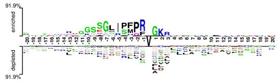
Figure 3.
Two sample logo of Valine amidation sites.
2.2. Sample Encoding
Almost all DNNs require data in the quantitative format before the neuron layers inside DNN process it. We applied a very basic quantitative encoding of PseAAC sequences, shown in Table 1, where 1st row displays the IUPAC symbols of amino acids, and corresponding entries in 2nd row show the integer used to represent the amino acid in the encoded sample. Since this encoding is the simplest possible amino acid numerical representation, it has no significant effects on the final results. The benchmark dataset was split into a training set of 968 PseAAC sequences (871 training sequences and 97 validation sequences) and a test set of 416 samples with a 70/30 ratio in the train set and test set. That is, for models training, 70% of the data was used, and the rest 30% was used for independent model testing. In all training and test sets, the initial 68/22 class ratio was preserved.

Table 1.
Encoding of amino acid used in this study.
2.3. Candidate Deep Model Training and Optimization
The training and optimization of DNN models for V-amide site prediction are described in this section. The study conducted experiments using well-known neural network architectures such as Fully Connected Neural Networks (FCNs), Convolutional Neural Networks (CNNs), and Recurrent Neural Networks (RNNs) with simple RNN units, Gated Recurrent Units (GRU), and Long Short-Term Memory (LSTM) units respectively. For optimization of DNN candidate models, we adopted the Randomized Hyperparameter search methodology of Bergstra et al. [44]. Randomized Hyperparameter search offers better hyperparameters for DNNs with the limited computational budget by performing a random search over large hyperparameter space. This is achieved by randomly sampling the hyperparameters from the space and evaluating the performance of models created using these parameters. For each DNN used to predict the V-Amide site, the following subparagraphs provide a brief introduction and architecture.
2.3.1. Standard Neural Network
Classic deep neural network architectures are standard neural networks or fully connected neural networks (FCNs). FCN is said to be fully connected because each neuron in the previous layer is connected to each neuron in the next layer. The FCN is intended to approximate the function. This function can be a classifier defined by and assigns a class label y to input x. The function of the FCN is to learn the parameters to offer the best possible approximation to for predicting class label y for each input x.
The FCN used for the V-Amide identification is shown in Figure 4. It is comprised of two dense layers, consisting of 20 and 10 rectified linear neurons (relu) respectively. The output layer of FCN was based on a single Sigmoid unit for binary classification. The architecture of FCN is shown in Table 2. To reduce negative logarithmic loss between actual and predicted class labels, this model was optimized using stochastic gradient descent (SGD) with a learning rate of 0.001. For training the FCN, only the training set was used, which was further divided into trainset and validation set with 80/20 partition ratio. FCN and other DNNs, used in this study, were never allowed to see the test set to ascertain the generalization capability of resulting V-amide prediction models. Once trained, the predictive model was independently tested on the test set, and performance was evaluated using standard performance evaluation metrics.
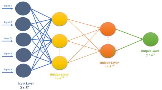
Figure 4.
Architecture of Standard Neural Network for V-Amide site identification.
Table 2.
Standard Neural Net (FCN) architecture for valine amidation identification.
2.3.2. Recurrent Neural Networks
The inherent weakness in conventional DNNs is the lack of sharing the weights learned by individual neurons, resulting in failure to identify similar patterns occurring at different positions of sequences [45]. RNN surmount this limitation by using a looping mechanism with time steps [46]. RNNs perform computations on a series of vectors using a recurrence of the from where f is an activation function, is a collection of hyperparameters used at each phase t and is input at timestep t.
This research utilizes three different RNN unit types to develop candidate models for the V-Amide prediction, which include simple RNN units, gated recurrent units (GRU), and long-short term memory unit (LSTM). In a simple RNN neuron, the parameters controlling the connections, from the input to the hidden layer, the horizontal connection between the activations and the hidden layer to the output layer, are shared. Forward pass in a simple RNN neuron can be formulated by following set of equations:
where <t> denotes the current time step, g expresses an activation function, represents input at timestep t, describes the bias, is activation output at timestep t, and denotes cumulative weights. This activation can be used to calculate the predictions at time t if desired. The architecture of the RNN model with simple RNN cells is shown in Table 3. This model makes use of an embedding layer to project each amino acid in vector space which converts the semantic relationships of amino acids, prevalent in sequences, to geometric relationships. These geometric relationships of sequence vectors are interpreted by following layers of DNN model to learn deep feature representations. These features are sent to the prediction output layer consisting of one sigmoid neuron. The architecture of three RNNs is shown in Figure 5 where the green circles show RNN units used in the network. Three different RNNs are used in this study comprising of Simple units, GRU units, and LSTM units respectively. In Figure 5, the red squares show different timesteps of the sequence being classified.
Table 3.
Simple RNN based model architecture for valine amidation identification.
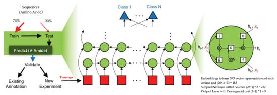
Figure 5.
Architecture of RNNs for V-Amide site identification.
Although the simple RNN units in many applications have shown promising results, they are prone to vanishing gradients and show limited capability to learn long-term dependencies in input sequences. This restriction on SimpleRNN cells is rectified via the GRU neurons [47] and the LSTM neurons [48].
The GRU cells, proposed by Cho et al. [47], are superior to the Simple RNN cell in reducing vanishing gradient problems. In each stage, the GRU cell uses the storage variable and contains summary of all the samples passed through the cell. At each timestep t, the GRU unit considers overwriting the contents of with a candidate value . This content overwriting is controlled by update gate , which decides whether or not the contents will be overwritten. Forward pass in GRU neuron can be described as follows:
In the above set of equations, and denote respective weights, the corresponding bias terms are illustrated by and , represents the input at timestep t, is the logistic regression function and represents activations at time step t. For V-Amide prediction, the RNN model architecture built with GRU is the same as the model based on SimpleRNN. Table 4 displays the architecture of GRU-based RNN model.
Table 4.
GRU-RNN based model architecture for valine amidation identification.
LSTM, proposed by Hochreiter et al. [48], is a more powerful generalization of GRU. Between GRU and LSTM neurons, the notable architectural differences are as follows:
- For computation, generic LSTM units do not use relevance gate .
- Instead of Update gate , LSTM units use two different gates including Output gate and Forget gate . Output gate monitors the exposure of the memory cell contents to compute activation outputs of LSTM unit for other hidden units in the network. Forget gate manages the amount of overwrite on to achieve , i.e., how much memory cell content needs to be forgotten for memory cell.
- In LSTM, the contents of the memory cell may not be equal to the activation which is contrary to GRU architecture.
With the exception of recurrent layer weights, the RNN model, built with the LSTM units, has the same architecture as that of SimpleRNN. The LSTM-based RNN model architecture for V-Amide prediction is shown in Table 5.
Table 5.
LSTM-RNN based model architecture for valine amidation identification.
2.3.3. Convolutional Neural Network
CNN is a neural network structure primarily designed to analyze data with complex spatial relationships like images or videos. CNN tries to learn a filter that can transform input data into the right output prediction. In addition to its capacity for handling large amounts of data, CNN can build local connections to learn feature maps, share training parameters among connections, and reduce dimensions using the subsampling operations. These characteristics help CNN to understand the spatial features of inputs despite their locality in the input data, a property known as location invariance.
The architecture of the V-Amide prediction model based on CNN is shown in Figure 6. The suggested CNN-based model was developed with an embedding layer, two convolution-maxpool blocks, a global averaging layer, and an output layer of sigmoid neuron. Every sample of the peptide x with a length of is encoded by the embedding layer in the form of tensor where is the representation vector of each amino acid residue in . First conv-maxpool block consists of a convolution layer having six 1-D convolution neurons and a maxpooling layer. The second conv-maxpool block uses a convolution layer having 16 1-D convolution neurons and a max-pooling layer. A Dropout layer is introduced between two conv-maxpool blocks to mitigate overfitting during training phase. By averaging the complete feature map, GlobalAveragePooling layer flattens the input into a one-dimensional array of 16 scalars used in the output layer to predict the markings. The output layer consists of a single sigmoid unit that performs binary classification. This detail is illustrated in Table 6 as well.
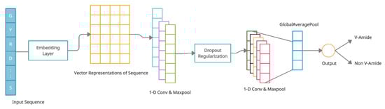
Figure 6.
Architecture of CNN for V-Amide site identification.
Table 6.
CNN based model architecture for valine amidation identification.
3. Results
This section explains the performance results of multiple DNN based predictors developed in this research to predict V-Amide site location. Notable evaluation metrics used in this study include receiver operating characteristics curve (ROC) curve, precision-recall curve and point metrics, including mean average precision (mAP), accuracy, F1 measurements, and Matthew’s correlation coefficient (MCC) to find the best DNN-based V-Amide prediction model. All models were evaluated on test data which was not used during the predictor training phase. This was done to ensure the fairness of results and to evaluate the generalization capability of predictors being evaluated. An overview of the model evaluation parameters used in this study is given in the following subsection, which illuminates adequate discussion of the results of the evaluation. To ensure fairness, all evaluation results come from independent test samples that were not used in the training phase of DNN based models.
3.1. Precision-Recall Curve and Mean Average Precision
For the evaluation of prediction models, precision and recall are essential indicators. Precision measures the relevance of the positive outcomes predicted by the model while recall measures the sensitivity of the model for positive samples. A high precision and recall rating imply that returned positive class predictions contain a high ratio of true positives (high Precision) while predicting the majority of positive class samples in the dataset (High Recall). Precision-Recall curve is achieved by plotting both of these metrics against each other and it evaluates the fraction of true positives among positive predictions [49]. In precision-recall space, the closer a score is to the perfect classification point (1,1), the better the predictor is and contrariwise.
Figure 7 shows the precision-recall curve of the candidate deep models for predicting the V-Amide PTM sites. As shown in Figure 7, the CNN-based predictive model performed best because it was closest to the perfect ranking point (1,1) in the precision-recall space. Worst performance was shown by the model trained using an FCN followed by the GRU-based prediction model.
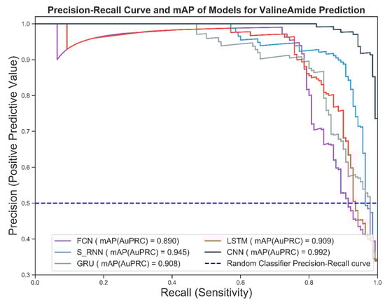
Figure 7.
Prec-Recall Curve and mAP scores achieved by DNN based V-amide identification models.
The mean average precision values for the four models are shown in the legend section of Figure 7. Mean average precision (mAP) provides a single-digit summary of precision-recall curves, which is the area under the precision-recall curve. The higher the value of the mAP, the better the practical performance and vice versa. As can be seen from Figure 7, the optimal mAP value of 0.992 is shown by the CNN-based model while simple RNN predictor showed runner-up performance. FCN based model turned out to be the least performing model followed by the GRU with values of 0.893 and 0.908, respectively.
3.2. Receiver Operating Characteristics and Area under ROC
The receiver operating characteristics curve (ROC) is a summary metric that represents the trade-off between the detection-rate (true positive rate) and the false alarm rate (false positive rate). According to Lasko et al. [50], ROC is a popular measure in Bioinformatics studies to evaluate predictor models. The ROC curve outlines the cost-benefit analysis of predictor where false-positive results depict costs, and true positives rate depicts the benefit of the classifier [51]. Some important points in the ROC space are (0,0), (1,1), and (0,1). The lowest point on the left (0,0) represents models that do not predict positive samples. The contrasting strategy, represented by a point (1,1), is to unconditionally classify each positive sample. The point (0,1) expresses the perfect classification with a false positive rate of 0 and a true positive rate score of 1. For predictors, the closer the curve is to the point (0,1) in ROC space, the better the performance of the corresponding predictor and vice versa.
The ROC curves of the predictive V-Amide models are shown in Figure 8. As shown in Figure 8, the ROC results confirm the results of the evaluation of the precision-recall curve. Here, too, the results of the CNN model dominate the results of the other models. Prediction models based on FCN, LSTM, RNN, and GRU gave slightly lower results. For model comparison, it may be useful to reduce the ROC curve to a single scalar value that shows the result of model performance is evaluated. One of these common methods is to calculate the area under the ROC curve called the AuC. AuC not only reduces the results of the ROC curve to a single value but is also statistically significant. This is because the AuC score corresponds to the probability of the evaluated model to rank randomly selected positive sample higher than randomly selected negative samples. The AuC values for the developed predictive model are shown in the legend section of Figure 8. The CNN-based predictive model indicates the highest AuC value with a value of 0.99. The model depicted the least score developed using FCN. This shows the capability of CNNs to learn better deep representations as compared to other DNN-based models. AuC scores of RNN based models were distributed between the two extremes, but it is notable to mention that all the results shown in Figure 8 have AUC value above 0.90. The comparison of the overall diagnostic accuracy of two models is frequently addressed by comparing the resulting paired AuCs using Delong’s method [52] of nonparametric comparison of two or more RoC curves. We used the fast implementation of Delong’s method by Sun et al. [53] to calculate the p-values by comparing each AuC with our best performing CNN based model. We also constructed the 95% Confidence interval using AuC for DNN based predictors developed in this study. Delong p-value scores and 95% confidence Intervals are shown in Table 7.
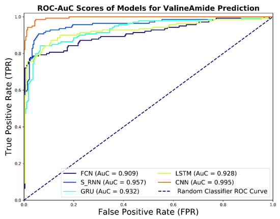
Figure 8.
ROC Curve and AUC Scores achieved by DNN based valine amidation identification models.
Table 7.
Comparison of the proposed approach with related literature contributions.
3.3. Accuracy, F1-Score, and Matthew’s Correlation
Accuracy, a popular classifier evaluation measure, highlights the fraction of results correctly classified by the model being evaluated. For independent testing, Figure 9 shows the results of the accuracy scores for the V-Amide prediction models developed in this study. As shown in Figure 9, the results are consistent with previously discussed evaluation metrics. CNN based prediction model showed an accuracy value of 95.9% while a minimum score of 89.4% is achieved by LSTM based model. Although accuracy is a standard measure, F1 results are used when an optimal precision and recall summary is required in the form of single scalar value.
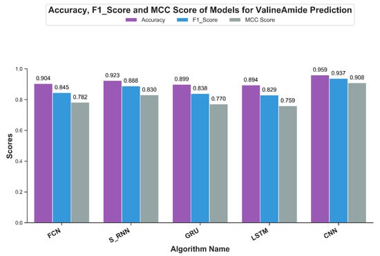
Figure 9.
Accuracy, F1-Measure and MCC achieved by DNN based valine amidation identification models.
Figure 9 shows the value F1 of the predictive V-Amide model. The F1 score also confirms the AuC and mAP scores. The best result in F1 was shown by the model CNN with a result of 93.7% and the second place from the simple RNN model with a result of F1 with a result of 88.8%. The LSTM based model gave a poor rating of 82.9%.
Matthews correlation coefficient (MCC) is a more accurate statistical metric that generates a high score only if good results were obtained in the prediction in all four groups of the confusion matrix [54]. MCC-scores of all DNN models are shown in Figure 9. The best MCC-score was achieved by CNN based model with a score of 0.908 while the second best score of 0.83 was shown by RNN model with simple neurons. Least score was shown by LSTM with the value of 0.75, making the CNN based model the clear choice for predicting V-Amide PTM sites.
4. Discussion
4.1. Comparison with Literature
For predicting the location of V-Amide sites in sequences, we were unable to find any research contribution, but we have compared the results with the two recently proposed predictors of amidation sites [8,23] shown in Table 7. The comparison is only shown for metrics available but essentially it shows the reader the promising results of proposed CNN based predictor. The results show that the proposed method surpasses the two previous methods for predicting V-Amide PTM sites.
As can be seen from Table 7, the proposed predictor performs better result using PseAAC sequences without requiring any complex and labor-intensive feature extraction. This is possible due to the inherent capability of DNNs to learn task-specific feature representations automatically.
4.2. Deep Feature Space Visualizations
To understand the deep feature representations, learned by the nonlinear transformation of iAmideV-Deep models, visualization of feature space serves as an important tool. For creating visualizations, we computed the output from penultimate layer of each trained model for test set sequences and projected this output to 2-D space using T-SNE, proposed by Maaten and Hinton [55]. T-SNE uses a nonlinear statistical approach to project data from higher dimensions to lower dimensions. This 2-D data was plotted based on class labels to understand the distribution of sequences belonging to both classes. For plotting the visualizations, we used matplotlib package of Python. The feature space of raw sequences is shown in Figure 10. As illustrated, raw sequences of V-amide are not that mixed up, to begin with, which means any decent binary classification model will be able to separate them comparatively easy compared to the case where both classes are completely jumbled up and inseparable. Nonlinear transformations of DNN models gradually segregate positive and negative data points and learn a more amenable representation to binary classification.
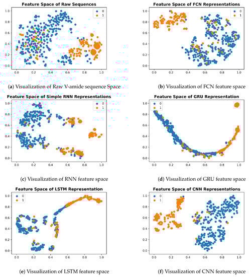
Figure 10.
Feature Space Visualizations of deep representations for positive and negative valine amide samples.
Deep representations for iAmideV-Deep models are shown in Figure 10. Figure 10b shows the deep feature representation learned by FCN. Figure 10c–e show that of RNN based models and Figure 10f shows the feature space of CNN representations. It can be deduced from the visual comparison of aforementioned figures that the best class separation is achieved by the CNN based representations and the output layer of CNN, which is a binary classifier, consume this deep feature representation to perform better predictions. It is relevant to mention that the feature representations used in this work are created from raw PseAAC sequences and do not require any domain expertise and human intervention. The data distribution of positive and negative samples in CNN representation is shown as violin plot and swarm plot in Figure 11 and Figure 12. As can be seen in aforementioned figures, the CNN model was able to learn the representation in which the positive and negative samples are sufficiently separated from each other enabling better V-amide site identification by output layer. The violin plot shown in Figure 12 further corroborate this conclusion by showing minimal overlap between the positive and negative samples in data distributions of different deep features of best performing CNN based model. Research contributions, shown in Table 7, use different feature extraction techniques which require domain knowledge and human intervention to predict the V-amide sites. Our approach automatically learns feature representation using stochastic gradient descent and removes the need to use expensive feature engineering process. Furthermore, the proposed deep models in this work demonstrate only the initial step towards DNN usage for V-amide PTM site prediction and additional research can build on work presented in this study to devise better DNN predictors for V-amide PTM site prediction.
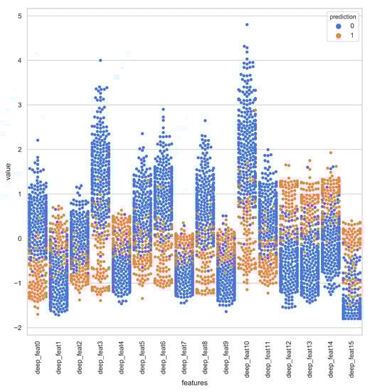
Figure 11.
Swarm-plot showing the data distribution of positive and negative samples in CNN deep representation.
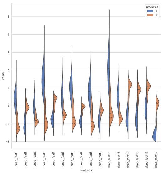
Figure 12.
Violin plot showing the data distribution of deep features learned by CNN Model.
4.3. Model Deployment as Web Service
The final step of Chou’s 5-step rule is to develop a web application for the public deployment of prediction model so that the latest advances become accessible to the collective research community. To this end, we developed a web application for our best performing CNN based prediction model, which can accept peptides and return the PTM sites along with corresponding length sequence of residues. Homepage of the aforementioned webserver is shown in Figure 13a. Figure 13b illustrates sequence submission procedure for computing amidation sites. Figure 13c demonstrates the result page showing the site and the corresponding length sequence of residues. Web service is temporarily deployed at http://3.19.14.13/. We believe our humble effort will improve the predictability of valine amidation and will be of service to the research community.
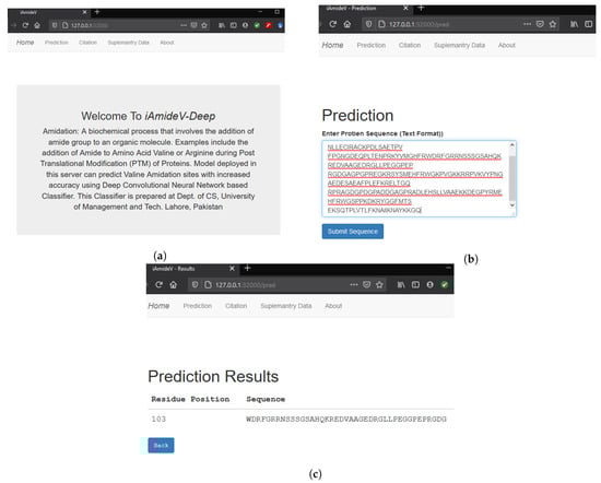
Figure 13.
iAmideV-Deep Webserver functionalities for identification of valine amidation. (a) Homepage of iAmideV-Deep Webserver. (b) Submission of protein sequence for amidation site prediction. (c) Valine Amidation site prediction results for the submitted sequence.
5. Conclusions
In this study, a new approach was proposed to identify valine amidation PTM sites, based on Chou’s Pseudo Amino Acid Composition (PseAAC) and deep neural networks. The study of the V-Amide mechanism is significant because amidated peptides are less sensitive to proteolytic degradation and have extended half-life in the bloodstream. Identifying in vitro, ex vivo, and in vivo can be tedious, time-consuming, and costly. We proposed a supplemental approach using well-known deep neural networks to learn efficient and task-specific representations and use these representations to develop predictor models. All DNN models, developed in this study, were evaluated using well-known model evaluation metrics with each other and literature contributions. Among the various DNNs, the convolution neural network learned best deep feature representation separating both classes and CNN based predictor achieved the best scores for all evaluation metrics, including an accuracy score of 95.9%. Owing to these results, it is concluded that the proposed model will help scientists to identify valine amidation in a very efficient and accurate way to understand the mechanism of this protein modification.
6. Limitation and Future Research
Like every experimental research work, our study also suffers from some limitations. The primary limitation of this study stems from the fact that deep neural networks mostly work like a black box and little information is available regarding the decision-making process of various neurons working together to make predictions. Although the research community is working on Explainable Artificial Intelligence (XAI), most research contributions in (XAI) including Grad-Cam and Activation maps are targeted towards computer vision and have very limited application on sequence based predictors. Future research in this area could overcome the XAI limitation discussed above. In the future, we seek to develop XAI for sequence based protein predictors to enhance their explainability.
Author Contributions
Conceptualization, S.N. and R.F.A.; methodology, S.N. and R.F.A.; software, S.N. and A.M.; validation, S.M.F. and R.F.A. formal analysis, S.M.F. and A.M. data curation, S.N. and R.F.A. writing—original draft preparation, S.N. and R.F.A. writing—review and editing, S.M.F. and A.M. visualization, S.N. and R.F.A. supervision, S.N. and S.M.F. project administration, S.N. and S.M.F. funding acquisition, S.M.F. All authors have read and agreed to the published version of the manuscript.
Funding
This research received no external funding.
Institutional Review Board Statement
Not applicable.
Informed Consent Statement
Not applicable.
Acknowledgments
The authors would like to acknowledge the support of Prince Sultan University, Saudi Arabia, for paying the Article Processing Charges (APC) of this publication.
Conflicts of Interest
The authors declare no conflict of interest.
References
- Arkhipenko, S.; Sabatini, M.T.; Batsanov, A.S.; Karaluka, V.; Sheppard, T.D.; Rzepa, H.S.; Whiting, A. Mechanistic insights into boron-catalysed direct amidation reactions. Chem. Sci. 2018, 9, 1058–1072. [Google Scholar] [CrossRef]
- Borah, G.; Borah, P.; Patel, P. Cp* Co (iii)-catalyzed ortho-amidation of azobenzenes with dioxazolones. Org. Biomol. Chem. 2017, 15, 3854–3859. [Google Scholar] [CrossRef] [PubMed]
- Chen, S.; Feng, B.; Zheng, X.; Yin, J.; Yang, S.; You, J. Iridium-catalyzed direct regioselective C4-amidation of indoles under mild conditions. Org. Lett. 2017, 19, 2502–2505. [Google Scholar] [CrossRef]
- Dorr, B.M.; Fuerst, D.E. Enzymatic amidation for industrial applications. Curr. Opin. Chem. Biol. 2018, 43, 127–133. [Google Scholar] [CrossRef]
- Lundberg, H.; Tinnis, F.; Zhang, J.; Algarra, A.G.; Himo, F.; Adolfsson, H. Mechanistic elucidation of zirconium-catalyzed direct amidation. J. Am. Chem. Soc. 2017, 139, 2286–2295. [Google Scholar] [CrossRef] [PubMed]
- Liang, D.; Yu, W.; Nguyen, N.; Deschamps, J.R.; Imler, G.H.; Li, Y.; MacKerell, A.D., Jr.; Jiang, C.; Xue, F. Iodobenzene-Catalyzed Synthesis of Phenanthridinones via Oxidative C–H Amidation. J. Org. Chem. 2017, 82, 3589–3596. [Google Scholar] [CrossRef] [PubMed]
- Mura, M.; Wang, J.; Zhou, Y.; Pinna, M.; Zvelindovsky, A.V.; Dennison, S.R.; Phoenix, D.A. The effect of amidation on the behaviour of antimicrobial peptides. Eur. Biophys. J. 2016, 45, 195–207. [Google Scholar] [CrossRef]
- Wang, T.; Zheng, W.; Wuyun, Q.; Wu, Z.; Ruan, J.; Hu, G.; Gao, J. PrAS: Prediction of amidation sites using multiple feature extraction. Comput. Biol. Chem. 2017, 66, 57–62. [Google Scholar] [CrossRef]
- Ortiz, G.X., Jr.; Hemric, B.N.; Wang, Q. Direct and selective 3-amidation of indoles using electrophilic N-[(benzenesulfonyl) oxy] amides. Org. Lett. 2017, 19, 1314–1317. [Google Scholar] [CrossRef]
- Yu, L.C.; Gu, J.W.; Zhang, S.; Zhang, X. Visible-Light-Promoted Tandem Difluoroalkylation–Amidation: Access to Difluorooxindoles from Free Anilines. J. Org. Chem. 2017, 82, 3943–3949. [Google Scholar] [CrossRef]
- Yu, X.; Yang, S.; Zhang, Y.; Guo, M.; Yamamoto, Y.; Bao, M. Intermolecular amidation of quinoline N-oxides with arylsulfonamides under metal-free conditions. Org. Lett. 2017, 19, 6088–6091. [Google Scholar] [CrossRef]
- Shi, P.; Wang, L.; Chen, K.; Wang, J.; Zhu, J. Co (III)-Catalyzed Enaminone-Directed C–H Amidation for Quinolone Synthesis. Org. Lett. 2017, 19, 2418–2421. [Google Scholar] [CrossRef] [PubMed]
- Rivera, H., Jr.; Dhar, S.; La Clair, J.J.; Tsai, S.C.; Burkart, M.D. An unusual intramolecular trans-amidation. Tetrahedron 2016, 72, 3605–3608. [Google Scholar] [CrossRef] [PubMed]
- Naseer, S.; Hussain, W.; Khan, Y.D.; Rasool, N. iPhosS(Deep)-PseAAC: Identify Phosphoserine Sites in Proteins using Deep Learning on General Pseudo Amino Acid Compositions via Modified 5-Steps Rule. IEEE/ACM Trans. Comput. Biol. Bioinform. 2020, 1. [Google Scholar] [CrossRef] [PubMed]
- Khan, Y.D.; Rasool, N.; Hussain, W.; Khan, S.A.; Chou, K.C. iPhosT-PseAAC: Identify phosphothreonine sites by incorporating sequence statistical moments into PseAAC. Anal. Biochem. 2018, 550, 109–116. [Google Scholar] [CrossRef] [PubMed]
- Butt, A.H.; Rasool, N.; Khan, Y.D. Predicting membrane proteins and their types by extracting various sequence features into Chou’s general PseAAC. Mol. Biol. Rep. 2018, 45, 2295–2306. [Google Scholar] [CrossRef] [PubMed]
- Naseer, S.; Hussain, W.; Khan, Y.D.; Rasool, N. Sequence-based Identification of Arginine Amidation Sites in Proteins Using Deep Representations of Proteins and PseAAC. Curr. Bioinform. 2021, 15, 937–948. [Google Scholar] [CrossRef]
- Akmal, M.A.; Rasool, N.; Khan, Y.D. Prediction of N-linked glycosylation sites using position relative features and statistical moments. PLoS ONE 2017, 12, e0181966. [Google Scholar] [CrossRef]
- Butt, A.H.; Rasool, N.; Khan, Y.D. A Treatise to Computational Approaches Towards Prediction of Membrane Protein and Its Subtypes. J. Membr. Biol. 2017, 250, 55–76. [Google Scholar] [CrossRef] [PubMed]
- Naseer, S.; Hussain, W.; Khan, Y.D.; Rasool, N. NPalmitoylDeep-PseAAC: A Predictor for N-Palmitoylation sites in Proteins using Deep Representations of Proteins and PseAAC via modified 5-steps rule. Curr. Bioinform. 2020, 15. [Google Scholar] [CrossRef]
- Hussain, W.; Khan, Y.D.; Rasool, N.; Khan, S.A.; Chou, K.C. SPalmitoylC-PseAAC: A sequence-based model developed via Chou’s 5-steps rule and general PseAAC for identifying S-palmitoylation sites in proteins. Anal. Biochem. 2019, 568, 14–23. [Google Scholar] [CrossRef]
- Song, J.; Wang, Y.; Li, F.; Akutsu, T.; Rawlings, N.D.; Webb, G.I.; Chou, K.C. iProt-Sub: A comprehensive package for accurately mapping and predicting protease-specific substrates and cleavage sites. Briefings Bioinform. 2019, 20, 638–658. [Google Scholar] [CrossRef]
- Zhao, S.; Yu, H.; Gong, X. Predicting protein amidation sites by orchestrating amino acid sequence features. JPhCS 2017, 887, 012052. [Google Scholar] [CrossRef]
- Yau, S.S.T.; Yu, C.; He, R. A Protein Map and Its Application. DNA Cell Biol. 2008, 27, 241–250. [Google Scholar] [CrossRef]
- Yu, C.; Cheng, S.Y.; He, R.L.; Yau, S.S.T. Protein map: An alignment-free sequence comparison method based on various properties of amino acids. Gene 2011, 486, 110–118. [Google Scholar] [CrossRef] [PubMed]
- Goodfellow, I.; Bengio, Y.; Courville, A. Deep Learning; MIT Press: Cambridge, MA, USA, 2016. [Google Scholar]
- Krizhevsky, A.; Sutskever, I.; Hinton, G.E. ImageNet Classification with Deep Convolutional Neural Networks. In Advances in Neural Information Processing Systems 25; Pereira, F., Burges, C.J.C., Bottou, L., Weinberger, K.Q., Eds.; Curran Associates, Inc.: Red Hook, NY, USA, 2012; pp. 1097–1105. [Google Scholar]
- Muneer, A.; Fati, S.M. Efficient and Automated Herbs Classification Approach Based on Shape and Texture Features using Deep Learning. IEEE Access 2020, 8, 196747–196764. [Google Scholar] [CrossRef]
- Sutskever, I.; Vinyals, O.; Le, Q.V. Sequence to sequence learning with neural networks. arXiv 2014, arXiv:1409.3215. [Google Scholar]
- Naseer, S.; Saleem, Y. Enhanced Network Intrusion Detection using Deep Convolutional Neural Networks. KSII Trans. Internet Inf. Syst. 2018, 12. [Google Scholar] [CrossRef]
- Naseer, S.; Ali, R.F.; Dominic, P.D.D.; Saleem, Y. Learning Representations of Network Traffic Using Deep Neural Networks for Network Anomaly Detection: A Perspective towards Oil and Gas IT Infrastructures. Symmetry 2020, 12, 1882. [Google Scholar] [CrossRef]
- LeCun, Y.; Bengio, Y.; Hinton, G. Deep learning. Nature 2015, 521, 436. [Google Scholar] [CrossRef]
- Chou, K.C. Using subsite coupling to predict signal peptides. Protein Eng. 2001, 14, 75–79. [Google Scholar] [CrossRef] [PubMed]
- Chou, K.C. Some remarks on protein attribute prediction and pseudo amino acid composition. J. Theor. Biol. 2011, 273, 236–247. [Google Scholar] [CrossRef] [PubMed]
- Cheng, X.; Xiao, X.; Chou, K.C. pLoc-mEuk: Predict subcellular localization of multi-label eukaryotic proteins by extracting the key GO information into general PseAAC. Genomics 2018, 110, 50–58. [Google Scholar] [CrossRef]
- Cheng, X.; Xiao, X.; Chou, K.C. pLoc-mHum: Predict subcellular localization of multi-location human proteins via general PseAAC to winnow out the crucial GO information. Bioinformatics 2017, 34, 1448–1456. [Google Scholar] [CrossRef]
- Jia, J.; Li, X.; Qiu, W.; Xiao, X.; Chou, K.C. iPPI-PseAAC (CGR): Identify protein-protein interactions by incorporating chaos game representation into PseAAC. J. Theor. Biol. 2019, 460, 195–203. [Google Scholar] [CrossRef] [PubMed]
- Wang, J.; Li, J.; Yang, B.; Xie, R.; Marquez-Lago, T.T.; Leier, A.; Hayashida, M.; Akutsu, T.; Zhang, Y.; Chou, K.C. Bastion3: A two-layer ensemble predictor of type III secreted effectors. Bioinformatics 2018, 35, 2017–2028. [Google Scholar] [CrossRef]
- Xiao, X.; Cheng, X.; Su, S.; Mao, Q.; Chou, K.C. pLoc-mGpos: Incorporate key gene ontology information into general PseAAC for predicting subcellular localization of Gram-positive bacterial proteins. Nat. Sci. 2017, 9, 330. [Google Scholar] [CrossRef]
- Naseer, S.; Hussain, W.; Khan, Y.D.; Rasool, N. Optimization of serine phosphorylation prediction in proteins by comparing human engineered features and deep representations. Anal. Biochem. 2021, 615, 114069. [Google Scholar] [CrossRef]
- The UniProt Consortium. UniProt: A worldwide hub of protein knowledge. Nucleic Acids Res. 2019, 47, D506–D515. [Google Scholar] [CrossRef] [PubMed]
- Chou, K.C. Prediction of signal peptides using scaled window. Peptides 2001, 22, 1973–1979. [Google Scholar] [CrossRef]
- Vacic, V.; Iakoucheva, L.M.; Radivojac, P. Two Sample Logo: A graphical representation of the differences between two sets of sequence alignments. Bioinformatics 2006, 22, 1536–1537. [Google Scholar] [CrossRef]
- Bergstra, J.; Bengio, Y. Random search for hyper-parameter optimization. J. Mach. Learn. Res. 2012, 13, 305. [Google Scholar]
- Bengio, Y.; Simard, P.; Frasconi, P. Learning Long-Term Dependencies with Gradient Descent is Difficult. IEEE Trans. Neural Netw. 1994, 5, 157–166. [Google Scholar] [CrossRef] [PubMed]
- Rumelhart, D.E.; Hinton, G.E.; Williams, R.J. Learning representations by back-propagating errors. Nature 1986, 323, 533. [Google Scholar] [CrossRef]
- Cho, K.; Van Merriënboer, B.; Bahdanau, D.; Bengio, Y. On the properties of neural machine translation: Encoder-decoder approaches. arXiv 2014, arXiv:1409.1259. [Google Scholar]
- Hochreiter, S.; Schmidhuber, J. Long Short-Term Memory. Neural Comput. 1997, 9, 1735–1780. [Google Scholar] [CrossRef]
- Saito, T.; Rehmsmeier, M. The Precision-Recall Plot Is More Informative than the ROC Plot When Evaluating Binary Classifiers on Imbalanced Datasets. PLoS ONE 2015, 10, e0118432. [Google Scholar] [CrossRef]
- Lasko, T.A.; Bhagwat, J.G.; Zou, K.H.; Ohno-Machado, L. The use of receiver operating characteristic curves in biomedical informatics. J. Biomed. Inform. 2005, 38, 404–415. [Google Scholar] [CrossRef]
- Fawcett, T. An introduction to ROC analysis. Pattern Recognit. Lett. 2006, 27, 861–874. [Google Scholar] [CrossRef]
- DeLong, E.R.; DeLong, D.M.; Clarke-Pearson, D.L. Comparing the areas under two or more correlated receiver operating characteristic curves: A nonparametric approach. Biometrics 1988, 44, 837–845. [Google Scholar] [CrossRef]
- Sun, X.; Xu, W. Fast Implementation of DeLong’s Algorithm for Comparing the Areas Under Correlated Receiver Operating Characteristic Curves. IEEE Signal Process. Lett. 2014, 21, 1389–1393. [Google Scholar] [CrossRef]
- Chicco, D.; Jurman, G. The advantages of the Matthews correlation coefficient (MCC) over F1 score and accuracy in binary classification evaluation. BMC Genom. 2020, 21, 6. [Google Scholar] [CrossRef] [PubMed]
- Maaten, L.V.D.; Hinton, G. Visualizing data using t-SNE. J. Mach. Learn. Res. 2008, 9, 2579–2605. [Google Scholar]


Publisher’s Note: MDPI stays neutral with regard to jurisdictional claims in published maps and institutional affiliations. |
© 2021 by the authors. Licensee MDPI, Basel, Switzerland. This article is an open access article distributed under the terms and conditions of the Creative Commons Attribution (CC BY) license (http://creativecommons.org/licenses/by/4.0/).