
An Improved Artificial Jellyfish Search Optimizer for Parameter Identification of Photovoltaic Models
by
 ,
,
Mohamed Abdel-Basset
1, 
Reda Mohamed
1,*,
Ripon K. Chakrabortty
2,
Michael J. Ryan
2 and
Attia El-Fergany
3
1
Department of Computer Science, Zagazig University, Shaibet an Nakareyah, Zagazig 44519, Egypt
2
Capability Systems Centre, School of Engineering and IT, UNSW Canberra 2052, Australia
3
Department of Electric Power & Machines, Zagazig University, Shaibet an Nakareyah, Zagazig 44519, Egypt
*
Author to whom correspondence should be addressed.
Energies 2021, 14(7), 1867; https://doi.org/10.3390/en14071867
Submission received: 13 February 2021
/
Revised: 14 March 2021
/
Accepted: 15 March 2021
/
Published: 27 March 2021
Abstract
:The optimization of photovoltaic (PV) systems relies on the development of an accurate model of the parameter values for the solar/PV generating units. This work proposes a modified artificial jellyfish search optimizer (MJSO) with a novel premature convergence strategy (PCS) to define effectively the unknown parameters of PV systems. The PCS works on preserving the diversity among the members of the population while accelerating the convergence toward the best solution based on two motions: (i) moving the current solution between two particles selected randomly from the population, and (ii) searching for better solutions between the best-so-far one and a random one from the population. To confirm its efficacy, the proposed method is validated on three different PV technologies and is being compared with some of the latest competitive computational frameworks. The numerical simulations and results confirm the dominance of the proposed algorithm in terms of the accuracy of the final results and convergence rate. In addition, to assess the performance of the proposed approach under different operation conditions for the solar cells, two additional PV modules (multi-crystalline and thin-film) are investigated, and the demonstrated scenarios highlight the utility of the proposed MJSO-based methodology.
1. Introduction
Recently, renewable energy sources (RESs) such as solar, wave, wind, and biomass play a vital role in addressing the cost, environmental pollution, global warming impact, and shortage of fossil fuels [1,2,3]. Among the RESs, solar energy has great potential to replace fossil fuels due to its ready availability and cleanliness [4]. The photovoltaic (PV) system is used widely worldwide to directly convert sunlight into electricity [5,6]. For efficient use, an accurate PV model is required for the optimal estimation of the unknown parameters based on the experimental data measured for PV systems under different operation conditions.
Meta-heuristic algorithms (MHAs) have been considered the optimal choice for addressing several real-world problems to identify better solutions in a reasonable time [7,8,9,10]. Therefore, MHAs have been widely used to generate the best values of the unidentified parameters of PV systems. Some of them will be surveyed in the rest of this section.
The Grasshopper optimization algorithm (GOA) improved using the levy flight strategy has been proposed for finding the unknown parameters of the PV models with the real data under different operating conditions. This proposed algorithm was abbreviated as LGOA [1]. The integration of levy flight strategy with the GOA guarantees diversity solutions and improves the exploitation and exploration operators in addition. The experimental findings show that LGOA was superior to GOA with respect to accuracy during estimating the unknown parameters of PV models. The marine predators algorithm has been proposed to solve the parameter extraction problem for the PV models by optimizing the Lambert W function as an objective function, namely MPALW [11]. This algorithm was compared with a number of well-established optimization algorithms for identifying the parameters of the single diode model (SDM) and double diode model (DDM) based on the empirical data of the Kyocera KC120-1 multi-crystalline PV module model. The outcomes proved the superiority of this algorithm in comparison with the others.
An approach based on modifying the teaching-learning-based optimization (TLBO) has been recently proposed to tackle the parameter identification problem of PV models under any irradiance and temperature level [12]. This modified TLBO (MTLBO) has been validated on five PV cells and modules and compared with a number of the recent robust optimization algorithms to see its efficacy. The experimental outcomes show that MLBO is the best.
A hybrid adaptive TLBO with differential evolution (DE), namely ATLDE, has recently been proposed for identifying accurately and efficiently the unknown parameters of the PV models [13]. ATLDE was applied for estimating the parameters of different PV models to verify their performance. Furthermore, it was compared with a number of well-established algorithms, which show that this algorithm is competitive in terms of accuracy and convergence speed. The social spider algorithm improved by replacing a number of the worst solutions at the beginning of each predefined period with other new ones in the search space was suggested for estimating the unidentified parameters of the PV models [14].
Furthermore, the learning search algorithm (LSA) was improved to identify the unknown parameters for solar cell models and PV models [15]. This improved LSA (ILSA) used the constant self-adjustment rate to improve the solutions diversity, the self-adaptive weight to guide the iterative direction during the optimization process, and the global optimal neighborhood perturbation and chaotic perturbation methods to avoid falling into local minima problem and improve final accuracy. The efficacy of ILSA was observed with some of the state-of-the-art algorithms on SDM, DDM, and PV modules. According to the experimental outcomes, it is proved that ILSA is the best with regard to accuracy and effectiveness.
An improved equilibrium optimizer (IEO) has been proposed for extracting the PV parameters of both SDM and DDM under different operational conditions [4]. The IEO used two novel strategies, namely linear reduction diversity technique (LRD) and local minima elimination method (MEM), to promote the exploitation and exploration capability for reaching better outcomes. IEO was verified on SDM and DDM for R.T.C. France commercial solar cells and three PV modules. In addition, it was also compared with some of the recently published state-of-the-art algorithms to observe its superiority.
Recently, MPA and SHADE algorithm were effectively combined for the optimal parameter values selection of SDM and DDM of monocrystalline, thin-film, and polycrystalline [16]. This algorithm was experimentally compared with some of the optimization techniques to check its effectiveness. The findings show that this algorithm is more effective. The Coyote Optimization Algorithm (COA) has been adapted for finding the unknown parameters of various PV solar cell and module models, including SDM, DDM, and third-diode models [17]. COA was validated on various PV modules using different operating conditions to check its stability and compared with a number of state-of-the-art techniques to see its ability in estimating the unknown parameters that fulfill lower value for the root mean square error (RMSE) with the experimental data. COA could have acceptable RMSE values of 7.64801 × , 7.59756 × , and 7.7547 × for DDM, TDM, and SDM.
The bat algorithm has been modified to estimate the unknown parameters of various PV models and is called the enhanced Lévy flight bat algorithm (ELBA) [18]. This modification is based on: improving the diversity of the solutions using a specific mathematical expression; using the levy flight to improve the local search ability; and balancing between exploration and exploitation using new equations to update specific control parameters. The experiments show that ELBA could be superior in terms of stability, effectiveness, convergence speed, robustness, and time. An enhanced TLBO (ETLBO) has been proposed to reach the unknown parameters of the PV cell and modules models, including SDM, DDM, and two real PV modules [19]. The ETLBO has been suggested to improve balancing between exploration and exploitation operators in the traditional TLBO by tuning the parameters which control in those two operators. After validation and comparison, it was proven that ETLBO was the best in terms of effectiveness and superiority.
A new parameter estimation technique called comprehensive learning Jaya algorithm (CLJAYA) has been proposed for PV models, which enhances the conventional Jaya algorithm by a mechanism called comprehensive learning used to promote its exploration capability for avoiding getting stuck in local minima and subsequently reaching better outcomes [20]. CLJAYA has been applied to extract the parameter values for three PV models: SDM, DDM, and PV module. As a result of validation and comparison with the Jaya algorithm, in addition to some of the other competitors, it was shown that CLJAYA was the best. A boosted Harris hawks optimization algorithm (BHHO) was improved by borrowing the exploration capability of the FPA and the powerful mutation strategy of the DE to accelerate convergence and exploration of other regions in the search space [21]. The real results proved the superiority of BHHO compared with the standard approach and other state-of-the-art methods.
A new meta-heuristic algorithm, namely generalized normal distribution optimization (GNDO) was applied to estimate the unknown parameters of the SDM, DDM, and PV module [22]. This algorithm was experimentally compared with some robust existing parameter estimation techniques to see its effectiveness. As a result of validation and comparison, GNDO could be competitive and superior in comparison with the others. The Harris hawks optimization algorithm has been reported to estimate the unidentified parameters of PV models [23]. Further, the slime mould algorithm (SMA) was proposed for estimating the parameters of SDM, DDM, TDM, and PV modules to see its efficacy under a number of function evaluations of 40,000 [24]. In addition, to validate the performance of SMA, the obtained outcomes were checked with the empirical data to see how far this algorithm could be near to the empirical data. More than that, it was also compared with a number of the meta-heuristic algorithms to see its superiority under various statistical metrics.
The opposition-based mechanism and the Nelder mead simplex method were integrated with the ant-lion optimization algorithm (ALO) to erase local minima, slow convergence speed, and imbalanced exploration and exploitation operators during selecting the optimal PV models parameters [25]. The opposition-based mechanism was used to strengthen the exploration operator of ALO to avoid entrapment into local minima. In addition, the Nelder–Mead simplex method was used for a smooth transfer from diversified search to an intensified one to increase the convergence speed for reaching better outcomes. This improved ALO (IALO) was validated by three solar cell and module models based on the experimental data to see if it can estimate the values of the parameters that minimize the error with empirical data or not. In addition, it was also compared with various well-established optimization algorithms to see its effectiveness and superiority. The experimental findings show that IALO was a promising technique for finding the unknown parameters of various PV models under standard operating conditions and various operating conditions.
In the same context, ALO was also improved to erase local minima and low convergence speed for estimating accurately and efficiently the unknown parameters of the PV cell models; this improved version was abbreviated as improved ALO [26]. This improved ALO used the tent chaotic map, chaotic search strategy, and adaptive parameter to get rid of those two problems mentioned above. Then, this algorithm was compared with the other existing algorithms for identifying the parameters of the PV cells under various irradiance and temperature levels. The experimental outcomes confirmed the superiority and effectiveness of this improved version. A new hybrid algorithm has been proposed for the optimal selection of the PV models’ parameters [27]. This hybrid algorithm combined the symbiotic differential evolution and the moth-flame optimization to utilize the advantages of each one to reach better accuracy for the PV models’ parameters estimation.
To estimate the parameters of the solar units of SDM and DDM, the JAYA algorithm was modified by integrating DE with the classical JAYA operator in addition to using a self-adaptive population size strategy to improve the exploration capability [28]. This algorithm was compared with different variants of JAYA, DE, and other algorithms to prove its superiority. Winner-leading competitive swarm optimizer with dynamic Gaussian mutation (WLCSODGM) was used for estimating the parameters of solar photovoltaic models [29]. WLCSODGM was validated to four different PV models and compared with 12 state-of-the-art algorithms. Many other algorithms have been recently proposed for tackling the parameters extraction problem of the solar cells, such as hybrid Jaya-NM algorithm [30], hybrid Firefly and Pattern Search Algorithms [31], genetic algorithm [32], diversification-enriched Harris hawks optimization with chaotic drifts [33], efficient salp swarm-inspired algorithm (SSA) [34], and modified SSA [35].
This paper proposes a new model that has a high ability to estimate the optimal parameters for PV systems (SDM and DDM) under the range of irradiance and temperature levels. The optimization model is based on an MHA called the artificial jellyfish search optimizer (JSO), inspired by the behaviors of jellyfish when searching for food. To accelerate the convergence of the proposed algorithm with preserving the diversity among the members of the population, a new method is proposed using the premature convergence strategy (PCS). This method works on preserving the diversity among the members of the population while accelerating the convergence toward the best solution based on two motions: (i) moving the current solution between two particles selected randomly from the population, and (ii) searching for better solutions between the best-so-far and a random solution from the population; those two motions are managed with a weight variable, also known as a control variable, which is generated randomly between 0 and 1. When the weight variable has a high value, then the motion between two particles selected randomly is high, but if it is small, then the premature method pays attention to the area between the best-so-far and the randomly selected one.
PCS can assist an MHA to accelerate its convergence towards the best-so-far solution by preserving the diversity among the members in order to avoid becoming trapped in local minima. By way of illustration, an MHA is based on two operators: exploration and exploitation. The former explores the search space of the problem far away from the best solution looking for the optimal solution; the latter focuses on the best-so-far solution in the hope of improving its quality. MHAs separate the exploration about the exploitation by giving emphasis to the exploration operator on the optimization process at the outset, but that will reduce the convergence toward the best-so-far solution by virtue of searching for a better solution in regions not near to the best-so-far solution that may be in an area near to the optimal solution. At the end of the optimization process, the exploitation capability increases and the exploration fades away forever. Therefore, if the best-so-far solution is a local minimum, the probability of reaching better is zero. We propose the PCS method to help an MHA to accelerate convergence while preserving the diversity among the population to avoid becoming trapped into local minima.
In this work, JSO is modified by PCS to accelerate its performance toward the best solution by reducing the possibility of falling into local minima; this proposed algorithm is called the modified JSO (MJSO). MJSO is validated to examine its efficacy on a solar cell called R.T.C.
France and two different PV units in addition to two other PV modules with different operating conditions. MJSO is also compared with a number of the well-known robust algorithms to show its superior performance on the different PV models in regard to accuracy and convergence speed.
The key contributions of the current work are (i) a novel application of MJSO to tackle the PV parameters’ identifications, (ii) proposing a new strategy to boost the performance of the basic JSO using PCS, and (iii) competitive results compared to selected extant MHA. The remainder of this paper is arranged as follows. Section 2 describes the different PV models: SDM, DDM, and PV module. Section 3 describes the standard artificial JSO. Section 4 explains the steps of the proposed algorithm for addressing the parameter estimation problem of the PV models: SDM and DDM. Section 5 shows the outcomes of the proposed approach along with comparisons to show its superiority. Section 6 explains the managerial implications and Section 7 provides conclusions and summarizes future work.
2. Mathematical Description of the Problem
This section describes the two most common mathematical models used to establish the I–V and P–V curve characteristics of solar cells and PV modules: SDM and DDM [36].
2.1. SDM
Figure 1 shows the equivalent electrical circuit of the SDM. indicates the photo-generated current [37]. is the diode current and computed as follows [38]:
where is the reverse saturation current of this diode, is the output voltage, is the series resistance, is the diode ideality factor, and is mathematically described as [24]:
where refers to the temperature degree of the junction in kelvin, is the Boltzmann constant (1.3806503 × 10⁻²³ J/K), and q defines the electron charge and is equal to 1.60217646 × 10⁻¹⁹ C.
is the shunt resistor current and formulated using the following equation [38]:
where indicates the shunt resistance. expresses the output of the SDM and mathematically formulated as follows [19,38]:
From the mathematical model, five unknown parameters () need to be optimized for better performance of the SDM.
2.2. DDM
The DDM model in Figure 2 is preferred at low irradiance levels because of its high accuracy. The equivalent circuit has two diodes in parallel so the DDM is mathematically described as [19]:
Equation (6) can be described in detail [19,38]:
where indicates the current of the first diode, while expresses the currents of the second diode, and and are the diodes’ ideality factors. From Equation (7), it is obvious that there are seven parameters (, , , , , , ) with unidentified values that need to be extracted accurately in order to optimize the performance of the solar cell DDM.
2.3. Photovoltaic (PV) Module
The mathematical models of the SDM and DDM of a PV module that consists of a compound of cells connected in series can be also formulated as Equations (5) and (7), where [39].
3. Artificial Jellyfish Search Optimizer
Chou and Troung proposed a new MHA based on the behavior of jellyfish in the ocean—the artificial jellyfish search optimizer (JSO) [40]. The behavior of the JSO for searching for food in the ocean involves: following the ocean current or movements inside the swarm, and using a time control mechanism to switch between these movements.
For the initialization steps, the authors in [40] observed several chaotic maps in addition to the typical random methods to find the better initialization way that will distribute the solutions within the search space of the problem accurately to accelerate the convergence and prevent stuck into local minima. After observation, JS is performed better under the logistic map [41] which is mathematically described as follows [40]:
is a vector that contains the logistic chaotic values of the th jellyfish. is an initial vector of jellyfish 0, generated randomly between 0 and 1. This vector is the start point that is relied on for generating the logistic chaotic values for the remainder of the jellyfish. is assigned a value of 4 according to [40]. After initialization, each solution is observed and the one with the best fitness value is chosen as the location with the most food . After that, the current location of each jellyfish is updated either toward the ocean current or motions inside the swarm based on the time control mechanism to switch between these two movements. In mathematical terms, the ocean current is formulated as follows [40]:
where is a vector generated randomly between 0 and 1, and is the element-by-element vector multiplication. is the distribution coefficient and based on the sensitivity analysis in [40], . is the mean of the population and is a random number between 0 and 1.
Movements inside the jellyfish swarm are divided into two motions: passive and active. In passive motion, the jellyfish move around their locations and the new location is given by the following formula [40]:
where is a random number between 0 and 1, and indicates the length of the motion around the current location. and are the upper and the lower bound of the search space of the problem, respectively. The active motion is mathematically formulated as follows [40]:
where is a vector that contains random values between 0 and 1. is used to determine the direction of the motion of the current jellyfish within the next generation and this motion is always in the direction to the location of the best food and formulated according to the following formula [40]:
where is the index of a jellyfish selected randomly, and indicates the fitness function. The time control mechanism is used to switch among the ocean current, passive and active motions, and includes a constant and a time control function mathematically formulated as follows [40]:
where is the current evaluation, is the maximum evaluation, and is a random number between 0 and 1. According to [40], the switching among the movements of the jellyfish under the time control mechanism is described in Figure 3. According to Figure 3 and Figure 4, the jellyfish follow the ocean current when , and move inside the swam otherwise with passive or active motion; passive motion is applied to the current jellyfish when a random number, , generated randomly between 0 and 1 is greater than (1 − ), otherwise, active motions are applied. Finally, Figure 4 describes the steps of the JSO.
4. Proposed Modified JSO (MJSO)
Within this section, the JSO is integrated with a novel method to promote exploration and exploitation capabilities when addressing the parameter extraction problem of the PV models based on SDM and DDM. This novel strategy called the PCS is related to a control variable to switch between the exploitation capability of the method to increase convergence toward the best solution and the exploration capability to reduce the likelihood of becoming trapped in local minima. The steps of the proposed algorithm are described in detail within the next subsections.
4.1. Initialization
At the start, the proposed algorithm uses a population consist of N solutions and each solution includes a number of the dimensions equal to the number of the unknown parameters that need to be optimized: five dimensions () for the SDM (see Table 1) and seven dimensions (, , , , , , ) for the DDM (see Table 2). Afterward, those dimensions are initialized using the logistic chaotic map, described previously within Section 3, within the search space of each unknown parameter shown later. After initialization, each solution is evaluated using the objective function (OF) described in the next section to determine the quality of each solution in comparison with the other solutions in addition to the solutions obtained within the next generations. In Table 1 and Table 2, the depiction of a solution initialized within the search boundaries of each unknown parameter given later in Table 3 for estimating the parameters of the SDM and DDM, respectively, is shown.
4.2. Evaluation Phase
The main target of solving the parameter extraction problem is to identify the values of the unknown parameters that minimize the error between the measured and simulated current data; this is the OF used with the proposed algorithm. The root mean squared error (RMSE) of the OF is computed between the measured current and the simulated current calculated by solving its non-linear equation using the Newton–Raphson method. In detail, the OF used with the proposed is described as follows [42,43]:
and are the measured and estimated currents, respectively. indicates the length of the measured data. is the estimated parameters of the th solution. is computed based on the extracted parameters represented in and using Newton–Raphson for solving Equations (5) and (7) as follows [42]:
is the derivative function of I as shown in Equation (16) for SDM. is the first derivative of dF with respect to I (see Equation (17) for SDM).
, , and for the DDM can be similarly formulated.
4.3. Premature Convergence Strategy (PCS)
From the description of the JSO in Section 3, it can be seen that the exploitation capability of the algorithm is low due to moving the current jellyfish inside the population which may not accelerate the convergence toward the best so-far solution, which may result in the algorithm taking a long time to reach a better solution. Moreover, the local exploration capability within the regions where the swarms are found is also weak and this may consume several iterations in searching within regions. Therefore, searching within the regions inside the swarm that maybe not be explored by any of the other jellyfish will help to reach better outcomes. This motivates the proposed PCS method to give improve the algorithm’s ability in the exploitation around the best-so-far solution when the control variable is a small and improved exploration around the swarm for reaching other regions when is high. Mathematically, the premature convergence method is:
where , , and are the indices of three solutions picked randomly from the population, r is the control parameter. This control parameter is a random number between 0 and 1 that is used to control in moving of the current solution; if it is small, the current solution will be moved to a location located between the best-so-far and to accelerate convergence; if it is high, the current one is updated based on two randomly selected solutions from the population to promote the ability of the algorithm to reach other regions. This method is then combined with the JS to modify its performance to reach better solutions in fewer evaluations. The MJSO method to include PCS is listed in Algorithm 1.
| Algorithm 1. The MJSO for the parameter estimation of PV models |
Output:
|
4.4. Time Complexity
The time complexity of the proposed algorithm: MJSO is based on two components:
- The big-O of the standard JSO.
- The big-O of the premature convergence method.
In the first, the big-O of JSO is based on three effective factors: the population size N, the number of the unknown parameters d, and maximum function evaluations , which is estimated as according to Algorithm 1. In the same context, the time complexity of the PCM is based on the same three factors and subsequently the same big-O. Hence, it is concluded that the time complexity of the proposed algorithm is of since the speed up of both the standard JSO and the premature convergence method is the same.
4.5. Advantages and Disadvantages
Before speaking about the advantage of the proposed algorithm, let us expose the strengths and weak points of the JSO. The conventional JSO is based on three behaviors: moving in the direction based on the ocean current and this behavior, as modeled in the algorithm, will encourage the exploration capability to search for the better position including more food; active motions inside the swarm, that will move the current solution in the direction of a solution selected randomly from the population and this might also help in exploring most regions within the search space, but if the optimal solution is near of the best-so-far solution, the algorithm might fail in reaching it; and passive motions, which will move the current solution randomly based on the step sizes generated randomly between the upper bound and lower bound of the optimization problem. All mentioned above shows that the conventional JSO encourages the exploration capability significantly and this is considered and advantage and disadvantage at the same time. Therefore, to overcome this disadvantage, the premature convergence method is proposed to promote the search in two directions: the first one is in the direction of the best-so-far solution to promote the exploitation capability, and the other is based on updating the current solution based on a step size generated using two solutions selected randomly from the population.
5. Results and Discussion
In this section, the performance of the proposed algorithm is validated on four different PV models: SDM on R.T.C. France cell, DDM on R.T.C. France cell, Photowatt-PWP201 module [44], and STP6-120/36 module [45]. In addition, to determine the stability of the proposed algorithm under different operation conditions, its performance is observed on two commercial PV systems based on SDM and DDM [46,47]. To confirm the superiority of the proposed algorithm, some of the recent parameter extraction algorithms are implemented using the same parameters values as in the cited paper to be compared with MJSO:
The experiments are conducted on a device with Intel(R) Core(TM) i7-4700MQ CPU @ 2.40 GHz, 32 GB RAM, Windows 10, and MATLAB R2019a to implement the algorithms. This part is structured as follows:
- Section 5.1 exposes the characteristics of the PV models.
- Section 5.2 shows the sensitivity analysis.
- Section 5.3 compares MJSO and JSO under the convergence speed.
- Section 5.4 gives the comparison of the R.T.C. France cell based on SDM.
- Section 5.5 announces a comparison of the R.T.C. France cell based on DDM.
- Section 5.6 gives a comparison of the Photowatt-PWP201 module.
- Section 5.7 announces a comparison of the STP6-120/36 module.
- Section 5.8 demonstrates the performance comparisons of the two commercial PV models.
5.1. Characteristics of Various Used PV Models
MJSO is validated on four well-known PV models: SDM on R.T.C. France cell, DDM on R.T.C. France cell, Photowatt-PWP201 module, and STP6-120/36 module due to using widely in the literature as test systems [20,24,51,52,53,54,55]. For the SDM and DDM, the current–voltage data are measured on a 57-mm diameter commercial silicon R.T.C. France solar cell under 1000 W/ at 33 °C [44]. To determine the performance of the proposed algorithm under different temperature levels, two different PV modules are used: the first is the Photowatt-PWP201 module compounded of 36 polycrystalline silicon cells connected in series and the current–voltage data are measured at 45 °C [44]. The second are the STP6-120/36 modules that also consist of 36 polycrystalline silicon cells connected in series and measured at 55 °C. The measured current–voltage data of the STP6-120/36 module are taken from [45,56]. The search boundaries of the unknown parameters are introduced in Table 3 as used in the other literature [39,48,57,58,59].
In addition, two solar modules—thin-film ST40 and mono-crystalline SM55 [12]—are used to determine the performance of the proposed algorithm under a range of operation conditions involving five irradiance levels: 200 W/, 400 W/, 600 W/, 800 W/, and 1000 W/ for both two modules and three temperature levels for mono-crystalline SM55 and four for thin-film ST40. The search boundary of Isc is specified according to the datasheet parameters of each module at the standard test condition (STC). Firstly, at the non-standard condition, is computed as described in [36]:
where and indicate the temperature and irradiance, respectively. refers to the short circuit current at STC, and expresses the temperature coefficient for the short circuit current [12]. Then, the upper bound and lower bounds of plus the other unknown parameters are assigned as described in Table 4. Further details in regard to the computation of other parameters such as , , , and band-energy voltage for the non-standard condition can be found in [12].
5.2. Parameter Setting
For all the algorithms used in these experiments, the maximum number of evaluations is set to 80,000. However, the population size may negatively affect the performance of the algorithms due to reducing the number of evaluations of each solution when the population size N is high. Therefore, to adjust the value of the parameter N, several values are used and the performance of the proposed approach under each value within 30 independent trials is observed and illustrated in Figure 5. According to this figure, values of 5, 22, 24, 23, 25, 40, and 50 for N degrade the performance of the algorithms. Meanwhile, the performance of the proposed approach reaches the maximum when N is between 8 and 17 while deteriorating a little between 18 and 21. Within the experiments, N is set to 17. Based on the original algorithm [40], the values of , , and are set to 3, 0.5, and 0.1, respectively. Table 5 reveals the parameter settings of the algorithms.
5.3. Comparison between JSO and MJSO in Term of Convergence Speed
The proposed MJSO algorithm is compared in Figure 6 with the standard algorithm: JSO according to the convergence speed under the different number of evaluations involving 80,000, 40,000, 10,000, and 5000. According to this figure, our proposed algorithm has a higher convergence speed in comparison with the JSO under a different number of evaluations. In detail, in Figure 6a–d, which picture the convergence curve of MJSO and JSO within 80,000 function evaluations for approximating the unknown parameters of SDM, DDM, Photowatt-PWP201, and STP6-120/36, MJSO could dramatically reach less RMSE value in comparison with the standard one and this obvious superiority is due to the premature convergence method, which helps in promoting the exploitation capability of the standard one with avoiding stuck into local minima. Furthermore, those two algorithms, MJSO and JSO, are compared under the other three maximum function evaluations to see if the performance of PCM is stable with the number of function evaluations or not. After picturing the convergence curve for those three maximum function evaluations within Figure 6e–h for 40,000 function evaluations, Figure 6i–l for 10,000 function evaluations, and Figure 6m,n for 5000 function evaluations, it is obvious that the improved version is the best and this shows the effectiveness of our proposed method.
5.4. Results for R.T.C France Cell Based on SDM
After running each algorithm 30 independent times, the extracted parameters that achieved the best RMSE for each algorithm within these runs are introduced in Table 6 with the corresponding RMSE. The table shows that ITLBO, CPMPSO, GNDO, and the proposed algorithm achieved the best value for RMSE, while JSO achieves a better RMSE for both WOA and SCA. The best, average, and worst values of the RMSE within these runs are arranged in Table 7, which shows that CPMPSO, GNDO, ITLBO, and MJSO can achieve the same average with a value of 0.0007730063. Five algorithms, including the proposed one, achieve lower average values for RMSE on SDM, so the convergence curve is used to determine which algorithm could reach the best RMSE in fewer. The parameters extracted by the MJSO are used to draw the I–V, P–V curves, and error values between all I estimated and I measured data points were computed using Equation (19) in Figure 7, which shows that MJSO identifies the parameter values that produce simulated data that are significantly harmonious with the measured for both I–V and P–V. The Time column in Table 7 shows the time, in seconds, needed by each algorithm. MJSO is in the fourth rank in terms of CPU time after SCA, WOA, and ITLBO.
5.5. Results for R.T.C. France Cell Based on DDM
The best-extracted parameter values and the corresponding RMSE over 30 independent runs on the DDM is introduced in Table 8 which shows that CPMPSO, GNDO, and MJSO attain the best parameter values with lower RMSE. Table 9 shows the best, average, worst, and SD obtained by each algorithm within the 30 independent runs. MJSO can be seen to outperform all the other algorithms in the average of RMSE with a value of 0.0007419371, while SCA is the worst with a value of 0.0480180357. Figure 8a,b show that the parameters estimated by MJSO produce a consistent match between the measured and estimated data for both the I–V and P–V characteristics. In addition, Figure 8c was presented to show the error value between each I estimated and I measured on R.T.C France cell based on DDM, which confirms that the selected parameter values by MJSO could significantly reach I estimated values so near that of the measured ones. This superiority in terms of RMSE and convergence curve is because of the PCM that could help in improving the exploitation capability of the proposed algorithm to reach better outcomes by avoiding stuck into local minima. Even now, our proposed algorithm is a strong alternative to the existing algorithms as elaborated in the current and previous sections.
5.6. Results for the PHOTOWATT-PWP201 Module
Table 10 announces the extracted parameters for the Photowatt-PWP201 module for the best RMSE within 30 independent trials of each algorithm. ITLBO, CPMPSO, GNDO, and MJSO are competitive on this model because all could reach the same smallest value of RMSE. Table 11 lists the stability of the algorithms over all the runs and ITLBO, CPMPSO, GNDO, and MJSO are competitive with the lowest values of the average values of RMSE. Figure 9 confirms that there is good consistency between the estimated and experimental data for MJSO for both the I–V and P–V principal characteristics and hence the error values between the I measured and estimated are so small as confirmed in Figure 9c.
5.7. Results for the STP6-120/36 Module
In this section, the performance among the algorithms on the STP6-120/36 module will be compared. Table 12 displays the best RMSE estimated by each algorithm with the corresponding extracted parameters. ITLBO, CPMPSO, GNDO, and MJSO have the lowest RMSE value. Table 13 shows the best, average, worst, SD, Rank, and time in seconds; ITLBO, CPMPSO, GNDO, and MJSO are competitive in terms of best, average, worst, while ITLBO is superior in terms of SD and time. Figure 10 confirms that the obtained parameters produce a consistent match between the measured and simulated characteristics.
Five algorithms, including the proposed one, achieve lower average values for RMSE on SDM, so the convergence curve is used to determine which algorithm could reach the best RMSE in fewer evaluations (see Figure 11). Figure 11a,b shows that the proposed algorithm has a high convergence in comparison to the other algorithms for R.T.C France. Figure 11b introduces the convergence curve of each algorithm on DDM, showing that MJSO converges faster. This superiority in terms of RMSE and convergence curve is because of the PCM that could help in improving the exploitation capability of the proposed algorithm to reach better outcomes by avoiding stuck into local minima. However, the convergence curve in Figure 11c shows that MJSO again converges the fastest. Once again, Figure 11d shows that the proposed algorithm converges fastest for STP6-120/36 based on SDM.
5.8. Observation with Experimental Data from the Manufactures’ Datasheets
To observe its practicability, the proposed algorithm is used in this section to find the values of the unknown parameters of DDM and SDM for two commercial PV models: mono-crystalline SM55, also called single crystalline silicon solar panels, and thin-film ST40. The experimental data for those PV modules are extracted from the I–V curves introduced by the manufacture’s datasheet at five different irradiance levels: 1000 W/, 800 W/, 600 W/, 400 W/, and 200 W/, and three temperature levels for SM55 and four for ST40. In terms of convergence, Figure 12, Figure 13, Figure 14, Figure 15, Figure 16, Figure 17, Figure 18, Figure 19 and Figure 20 illustrate without any doubts that the proposed algorithm reaches the best solution in fewer iterations and are presented to show the error value between each I measured and I estimated on SM55 and ST40, respectively, at varied temperature levels to show how far our proposed could accurately estimate the unknown parameters. The latter mentioned is detailed as follows:
A. Case Study 1: Single Diode Model
In this section, the efficacy of MJSO is observed on SM55 and for ST40 based on SDM under different operation conditions. Table 14 contains the average, worst, best, and SD of the RMSE obtained by ITLBO, GNDO, and MJSO at various irradiance levels with a temperature of 25 °C through 30 independent trials. It can be observed that all the algorithms achieve the same value within 30 independent runs. Regarding Table 15, it contains the best, worst, average, and SD of the RMSE obtained by ITLBO, GNDO, and MJSO at various temperature levels with an irradiance level of 1000 W/ through 30 independent trials. In addition, it can be observed that all the algorithms achieve the same value within 30 independent runs. Figure 12 and Figure 18 establish the consistency between the measured and estimated data for both the I–V and P–V curves confirming the accuracy of the obtained parameters by MJSO for both ST40 and SM55 at various temperature levels. Figure 14 and Figure 16 also indicate the accuracy of the estimated parameters by MJSO for those two modules at various irradiance levels. In addition, Figure 13 and Figure 21 are presented to show the error value between each I measured and I estimated on SM55 and ST40, respectively, at varied temperature levels to show how far our proposed could accurately estimate the unknown parameters. After inspecting those figures, it is obvious that the proposed algorithm could accurately estimate the parameter values that minimize the error values between the measured and estimated data and this reflects the superior performance of our proposed algorithm. In addition, Figure 15 and Figure 17 depict the error value between each I measured and I estimated on SM55 and ST40 at different irradiance levels, respectively. Those figures show that the error values between the measured and estimated I are so small and this reflects the high-ability of our proposed algorithm in accurately estimating the unknown parameters. Table 16 exposes the estimated parameters with its corresponding RMSE obtained by MJSO under different G and T for ST40 and SM55 modules based on SDM.
B. Case Study 2: Double Diode Model
After running each algorithm 30 independent runs on the SM55 module and ST40 module based on the DDM with experimental data extracted at various irradiance levels (G), the best, average, worst, and SD of the RMSE obtained within those runs are introduced in Table 17. To the best of our knowledge, ITLBO and GNDO are the best two-parameter extraction models developed to date. MJSO is competitive with those two algorithms, but the convergence curves in Figure 21, Figure 22, Figure 23, Figure 24, Figure 25, Figure 26, Figure 27, Figure 28 and Figure 29 illustrate that the proposed algorithm converges faster and confirm the consistency between the estimated and measured data at various conditions. More specifically, Figure 23 and Figure 25 confirm the consistency between the estimated and measured data, for both the SM55 module and ST40, respectively. More than that, Figure 24 and Figure 28 are presented to picture the error values between the I estimated and I measured on SM55 and ST40, respectively, at varied irradiance levels to show the ability of our proposed algorithm in estimating the near-optimal values of the unknown parameters that minimize those error values. By observation, it is clear that the proposed algorithm could significantly minimize the error value between the measured and estimated.
Under different temperature levels and G = 1000 W/m2, Table 18 provides the best, average, worst, and SD of the RMSE extracted within 30 independent trials. MJSO is competitive with GNDO at temperature levels of 25 °C for the SM55 module, and superior at all the other levels for both modules. Figure 21 and Figure 27 confirm the extracted parameters produce consistent results between the measured and estimated data with different T for both I–V and P–V curves. In addition, to show to how far the outcomes of our proposed algorithm are near of the I measured, Figure 24 and Figure 26 are presented to show the error value between each I estimated and I measured on SM55 and ST40 at varied temperature levels. After inspecting those figures, it was obvious that the proposed algorithm could significantly minimize the error value between the I estimated and I measured for all 25 datapoints. The estimated parameters with the corresponding RMSE obtained under the proposed algorithms for those two modules based on DDM at various G and T are pictured in Table 19.
6. Managerial Implications
Based on the above experiments, a number of observations can be made regarding the implications related to the proposed models. This research proposes a new alternative model with high efficiency for estimating the parameters of the PV systems. According to the results of this model, it has a high ability for efficiently and accurately finding the unidentified parameters of the SDM and DDM models under various operational conditions in comparison with the recent robust parameter extraction model in terms of the accuracy of the final results, especially for DDM, and the convergence speed. In addition, under various operating conditions on two commercial models, SM55 and ST40 based on both SDM and DDM, the model is able to adapt itself to estimate the optimal values of the unknown parameters, outperforming the other algorithms in particular for the DDM. Therefore, MJSO is a straightforward model in terms of understanding and implementation, in addition to its efficacy for estimating the parameters of the PV models efficiently and accurately under any conditions in a reasonable time. Consequently, MJSO is a good alternative for estimating the unidentified parameters of the PV systems under different operational conditions.
7. Conclusions
This paper presents an effective parameter extraction for PV models (i.e., SDM and DDM) based on the JSO integrated with a novel PCS; namely MJSO. The PCS is a simple approach to searching within the search space, preserving the diversity among the solutions while promoting the convergence speed toward the best solution based on two predefined motions. The efficiency of the proposed approach is justified on three different PV systems including SDM and DDM for R.T.C France cell, and other PV modules with different solar technologies. After validating the proposed approach, it is compared with several recently published algorithms for solving the same problem under the same conditions for fair comparisons. The proposed algorithm has shown to be superior to the others based on the outcomes and convergence speed. By way of quantitative example, for the R.T.C France cell based on SDM, MJSO could achieve an average RMSE value of 7.730063E-3 A, which is also achieved by some of the other algorithms but with slow convergence speed. Further, for DDM and the R.T.C France cell, MJSO minimizes the RMSE until an average value of 7.419372E-3 A and outperformed the other methods. Further, two PV modules at different irradiance and temperature levels (mono-crystalline and thin-film) are used as examples of PV technologies to confirm the superiority of the proposed approach under different operating conditions. Future work involves checking the performance of this method with one of the other robust optimization algorithms seeking better outcomes for extracting the parameter values of the solar cell efficiently and accurately.
Author Contributions
Conceptualization, M.A.-B. and R.M.; methodology, A.E.-F.; software, M.A.-B. and R.M.; validation, M.A.-B. and R.M.; formal analysis and investigation, A.E.-F.; resources, R.K.C. and M.J.R.; data curation, M.A.-B. and R.M.; writing—original draft preparation, M.A.-B. and R.M.; writing—review and editing, R.K.C. and M.J.R.; visualization, R.K.C. and M.J.R.; supervision, A.E.-F.; project administration, R.K.C. and M.J.R.; funding acquisition, R.K.C. and M.J.R. All authors have read and agreed to the published version of the manuscript.
Funding
This research has no funding source.
Institutional Review Board Statement
Not applicable.
Informed Consent Statement
Not applicable.
Conflicts of Interest
The authors declare that there is no conflict of interest in the research.
References
- Mokeddem, D. Parameter Extraction of Solar Photovoltaic Models Using Enhanced Levy Flight Based Grasshopper Optimization Algorithm. J. Electr. Eng. Technol. 2021, 16, 171–179. [Google Scholar] [CrossRef]
- Nacar, M.; Özer, E.; Yılmaz, A.E. A Six Parameter Single Diode Model for Photovoltaic Modules. J. Sol. Energy Eng. 2021, 143, 011012. [Google Scholar] [CrossRef]
- Abdel-Basset, M.; El-Shahat, D.; Chakrabortty, R.K.; Ryan, M. Parameter estimation of photovoltaic models using an improved marine predators algorithm. Energy Convers. Manag. 2021, 227, 113491. [Google Scholar] [CrossRef]
- Abdel-Basset, M.; Mohamed, R.; Mirjalili, S.; Chakrabortty, R.K.; Ryan, M.J. Solar photovoltaic parameter estimation using an improved equilibrium optimizer. Sol. Energy 2020, 209, 694–708. [Google Scholar] [CrossRef]
- Parida, B.; Iniyan, S.; Goic, R. A review of solar photovoltaic technologies. Renew. Sustain. Energy Rev. 2011, 15, 1625–1636. [Google Scholar] [CrossRef]
- Bechouat, M.; Younsi, A.; Sedraoui, M.; Soufi, Y.; Yousfi, L.; Tabet, I.; Touafek, K. Parameters identification of a photovoltaic module in a thermal system using meta-heuristic optimization methods. Int. J. Energy Environ. Eng. 2017, 8, 331–341. [Google Scholar] [CrossRef] [Green Version]
- Abdel-Basset, M.; Mohamed, R.; Elhoseny, M.; Bashir, A.K.; Jolfaei, A.; Kumar, N. Energy-aware marine predators algorithm for task scheduling in IoT-based fog computing applications. IEEE Trans. Ind. Inform. 2020, in press. [Google Scholar] [CrossRef]
- Abdel-Basset, M.; Mohamed, R.; Chakrabortty, R.K.; Ryan, M.; Mirjalili, S. New binary marine predators optimization algorithms for 0–1 knapsack problems. Comput. Ind. Eng. 2020, 151, 106949. [Google Scholar] [CrossRef]
- Abdel-Basset, M.; Mohamed, R.; Sallam, K.M.; Chakrabortty, R.K.; Ryan, M.J. An Efficient-Assembler Whale Optimization Algorithm for DNA Fragment Assembly Problem: Analysis and Validations. IEEE Access 2020, 8, 222144–222167. [Google Scholar] [CrossRef]
- Kotte, S.; Pullakura, R.K.; Injeti, S.K. Optimal multilevel thresholding selection for brain MRI image segmentation based on adaptive wind driven optimization. Measurement 2018, 130, 340–361. [Google Scholar] [CrossRef]
- Ridha, H.M. Parameters extraction of single and double diodes photovoltaic models using Marine Predators Algorithm and Lambert W function. Sol. Energy 2020, 209, 674–693. [Google Scholar] [CrossRef]
- Abdel-Basset, M.; Mohamed, R.; Chakrabortty, R.K.; Sallam, K.; Ryan, M.J. An efficient teaching-learning-based optimization algorithm for parameters identification of photovoltaic models: Analysis and validations. Energy Convers. Manag. 2021, 227, 113614. [Google Scholar] [CrossRef]
- Li, S.; Gong, W.; Wang, L.; Yan, X.; Hu, C. A hybrid adaptive teaching–learning-based optimization and differential evolution for parameter identification of photovoltaic models. Energy Convers. Manag. 2020, 225, 113474. [Google Scholar] [CrossRef]
- Kashefi, H.; Sadegheih, A.; Mostafaeipour, A.; Omran, M.M. Parameter identification of solar cells and fuel cell using improved social spider algorithm. Compel-Int. J. Comput. Math. Electr. Electron. Eng. 2020, in press. [Google Scholar] [CrossRef]
- Huang, T.; Zhang, C.; Ouyang, H.; Luo, G.; Li, S.; Zou, D. Parameter Identification for Photovoltaic Models Using an Improved Learning Search Algorithm. Ieee Access 2020, 8, 116292–116309. [Google Scholar] [CrossRef]
- Naraharisetti, J.N.L.; Devarapalli, R.; Bathina, V. Parameter extraction of solar photovoltaic module by using a novel hybrid marine predators–success history based adaptive differential evolution algorithm. Energy Sources Part A Recovery Util. Environ. Eff. 2020, 1–23, in press. [Google Scholar]
- Diab, A.A.Z.; Sultan, H.M.; Do, T.D.; Kamel, O.M.; Mossa, M.A. Coyote optimization algorithm for parameters estimation of various models of solar cells and PV modules. Ieee Access 2020, 8, 111102–111140. [Google Scholar] [CrossRef]
- Deotti, L.M.P.; Pereira, J.L.R.; da Silva Júnior, I.C. Parameter extraction of photovoltaic models using an enhanced Lévy flight bat algorithm. Energy Convers. Manag. 2020, 221, 113114. [Google Scholar] [CrossRef]
- Ramadan, A.; Kamel, S.; Korashy, A.; Yu, J. Photovoltaic cells parameter estimation using an enhanced teaching–learning-based optimization algorithm. Iran. J. Sci. Technol. Trans. Electr. Eng. 2020, 44, 767–779. [Google Scholar] [CrossRef]
- Zhang, Y.; Ma, M.; Jin, Z. Comprehensive learning Jaya algorithm for parameter extraction of photovoltaic models. Energy 2020, 211, 118644. [Google Scholar] [CrossRef]
- Ridha, H.M.; Heidari, A.A.; Wang, M.; Chen, H. Boosted mutation-based Harris hawks optimizer for parameters identification of single-diode solar cell models. Energy Convers. Manag. 2020, 209, 112660. [Google Scholar] [CrossRef]
- Zhang, Y.; Jin, Z.; Mirjalili, S. Generalized normal distribution optimization and its applications in parameter extraction of photovoltaic models. Energy Convers. Manag. 2020, 224, 113301. [Google Scholar] [CrossRef]
- Sharma, A.; Saxena, A.; Shekhawat, S.; Kumar, R.; Mathur, A. Solar Cell Parameter Extraction by Using Harris Hawks Optimization Algorithm. In Bio-Inspired Neurocomputing; Springer: Berlin/Heidelberg, Germany, 2020; pp. 349–379. [Google Scholar]
- Kumar, C.; Raj, T.D.; Premkumar, M.; Raj, T.D. A new stochastic slime mould optimization algorithm for the estimation of solar photovoltaic cell parameters. Optik 2020, 223, 165277. [Google Scholar] [CrossRef]
- Wang, M.; Zhao, X.; Heidari, A.A.; Chen, H. Evaluation of constraint in photovoltaic models by exploiting an enhanced ant lion optimizer. Sol. Energy 2020, 211, 503–521. [Google Scholar] [CrossRef]
- Wu, Z.-q.; Xie, Z.-k.; Liu, C.-y. An improved lion swarm optimization for parameters identification of photovoltaic cell models. Trans. Inst. Meas. Control 2020, 42, 1191–1203. [Google Scholar] [CrossRef]
- Thawkar, S. A hybrid model using teaching–learning-based optimization and Salp swarm algorithm for feature selection and classification in digital mammography. J. Ambient Intell. Humaniz. Comput. 2021, 1–16, In press. [Google Scholar]
- Luu, T.V.; Nguyen, N.S. Parameters extraction of solar cells using modified JAYA algorithm. Optik 2020, 203, 164034. [Google Scholar] [CrossRef]
- Xiong, G.; Zhang, J.; Shi, D.; Zhu, L.; Yuan, X.; Tan, Z. Winner-leading competitive swarm optimizer with dynamic Gaussian mutation for parameter extraction of solar photovoltaic models. Energy Convers. Manag. 2020, 206, 112450. [Google Scholar] [CrossRef]
- Luo, X.; Cao, L.; Wang, L.; Zhao, Z.; Huang, C. Parameter identification of the photovoltaic cell model with a hybrid Jaya-NM algorithm. Optik 2018, 171, 200–203. [Google Scholar] [CrossRef]
- Beigi, A.M.; Maroosi, A. Parameter identification for solar cells and module using a Hybrid Firefly and Pattern Search Algorithms. Sol. Energy 2018, 171, 435–446. [Google Scholar] [CrossRef]
- Zhang, Z.; Huang, S.; Chen, Y.; Wei, W. Key Parameter Identification and Optimization of Photovoltaic Power Plants Based on Genetic Algorithm. J. Phys. Conf. Ser. 2020, 1449, 12044. [Google Scholar] [CrossRef] [Green Version]
- Chen, H.; Jiao, S.; Wang, M.; Heidari, A.A.; Zhao, X. Parameters identification of photovoltaic cells and modules using diversification-enriched Harris hawks optimization with chaotic drifts. J. Clean. Prod. 2020, 244, 118778. [Google Scholar] [CrossRef]
- Abbassi, R.; Abbassi, A.; Heidari, A.A.; Mirjalili, S. An efficient salp swarm-inspired algorithm for parameters identification of photovoltaic cell models. Energy Convers. Manag. 2019, 179, 362–372. [Google Scholar] [CrossRef]
- Abbassi, A.; Abbassi, R.; Heidari, A.A.; Oliva, D.; Chen, H.; Habib, A.; Jemli, M.; Wang, M. Parameters identification of photovoltaic cell models using enhanced exploratory salp chains-based approach. Energy 2020, 198, 117333. [Google Scholar] [CrossRef]
- Xu, S.; Wang, Y. Parameter estimation of photovoltaic modules using a hybrid flower pollination algorithm. Energy Convers. Manag. 2017, 144, 53–68. [Google Scholar] [CrossRef]
- Tan, Y.T.; Kirschen, D.S.; Jenkins, N. A model of PV generation suitable for stability analysis. Ieee Trans. Energy Convers. 2004, 19, 748–755. [Google Scholar] [CrossRef]
- Benkercha, R.; Moulahoum, S.; Taghezouit, B. Extraction of the PV modules parameters with MPP estimation using the modified flower algorithm. Renew. Energy 2019, 143, 1698–1709. [Google Scholar] [CrossRef]
- Gong, W.; Cai, Z. Parameter extraction of solar cell models using repaired adaptive differential evolution. Sol. Energy 2013, 94, 209–220. [Google Scholar] [CrossRef]
- Chou, J.-S.; Truong, D.-N. A novel metaheuristic optimizer inspired by behavior of jellyfish in ocean. Appl. Math. Comput. 2021, 389, 125535. [Google Scholar]
- Gandomi, A.H.; Yang, X.-S.; Talatahari, S.; Alavi, A.H. Firefly algorithm with chaos. Commun. Nonlinear Sci. Numer. Simul. 2013, 18, 89–98. [Google Scholar] [CrossRef]
- Nunes, H.; Pombo, J.; Mariano, S.; Calado, M.; De Souza, J.F. A new high performance method for determining the parameters of PV cells and modules based on guaranteed convergence particle swarm optimization. Appl. Energy 2018, 211, 774–791. [Google Scholar] [CrossRef]
- Laudani, A.; Fulginei, F.R.; Salvini, A. High performing extraction procedure for the one-diode model of a photovoltaic panel from experimental I–V curves by using reduced forms. Sol. Energy 2014, 103, 316–326. [Google Scholar] [CrossRef]
- Easwarakhanthan, T.; Bottin, J.; Bouhouch, I.; Boutrit, C. Nonlinear minimization algorithm for determining the solar cell parameters with microcomputers. Int. J. Sol. Energy 1986, 4, 1–12. [Google Scholar] [CrossRef]
- Tong, N.T.; Pora, W. A parameter extraction technique exploiting intrinsic properties of solar cells. Appl. Energy 2016, 176, 104–115. [Google Scholar] [CrossRef] [Green Version]
- Liang, J.; Ge, S.; Qu, B.; Yu, K.; Liu, F.; Yang, H.; Wei, P.; Li, Z. Classified perturbation mutation based particle swarm optimization algorithm for parameters extraction of photovoltaic models. Energy Convers. Manag. 2020, 203, 112138. [Google Scholar] [CrossRef]
- Merchaoui, M.; Sakly, A.; Mimouni, M.F. Particle swarm optimisation with adaptive mutation strategy for photovoltaic solar cell/module parameter extraction. Energy Convers. Manag. 2018, 175, 151–163. [Google Scholar] [CrossRef]
- Li, S.; Gong, W.; Yan, X.; Hu, C.; Bai, D.; Wang, L.; Gao, L. Parameter extraction of photovoltaic models using an improved teaching-learning-based optimization. Energy Convers. Manag. 2019, 186, 293–305. [Google Scholar] [CrossRef]
- Elazab, O.S.; Hasanien, H.M.; Elgendy, M.A.; Abdeen, A.M. Parameters estimation of single-and multiple-diode photovoltaic model using whale optimisation algorithm. Iet Renew. Power Gener. 2018, 12, 1755–1761. [Google Scholar] [CrossRef]
- Mirjalili, S. SCA: A sine cosine algorithm for solving optimization problems. Knowl. Based Syst. 2016, 96, 120–133. [Google Scholar] [CrossRef]
- Premkumar, M.; Babu, T.S.; Umashankar, S.; Sowmya, R. A new metaphor-less algorithms for the photovoltaic cell parameter estimation. Optik 2020, 208, 164559. [Google Scholar] [CrossRef]
- Lin, P.; Cheng, S.; Yeh, W.; Chen, Z.; Wu, L. Parameters extraction of solar cell models using a modified simplified swarm optimization algorithm. Sol. Energy 2017, 144, 594–603. [Google Scholar] [CrossRef]
- Kler, D.; Sharma, P.; Banerjee, A.; Rana, K.; Kumar, V. PV cell and module efficient parameters estimation using Evaporation Rate based Water Cycle Algorithm. Swarm Evol. Comput. 2017, 35, 93–110. [Google Scholar] [CrossRef]
- Gnetchejo, P.J.; Essiane, S.N.; Ele, P.; Wamkeue, R.; Wapet, D.M.; Ngoffe, S.P. Enhanced vibrating particles system Algorithm for parameters estimation of photovoltaic system. J. Power Energy Eng. 2019, 7, 1. [Google Scholar] [CrossRef] [Green Version]
- Ebrahimi, S.M.; Salahshour, E.; Malekzadeh, M.; Gordillo, F. Parameters identification of PV solar cells and modules using flexible particle swarm optimization algorithm. Energy 2019, 179, 358–372. [Google Scholar] [CrossRef]
- Gao, X.; Cui, Y.; Hu, J.; Xu, G.; Wang, Z.; Qu, J.; Wang, H. Parameter extraction of solar cell models using improved shuffled complex evolution algorithm. Energy Convers. Manag. 2018, 157, 460–479. [Google Scholar] [CrossRef]
- Yu, K.; Liang, J.; Qu, B.; Cheng, Z.; Wang, H. Multiple learning backtracking search algorithm for estimating parameters of photovoltaic models. Appl. Energy 2018, 226, 408–422. [Google Scholar] [CrossRef]
- Yu, K.; Liang, J.; Qu, B.; Chen, X.; Wang, H. Parameters identification of photovoltaic models using an improved JAYA optimization algorithm. Energy Convers. Manag. 2017, 150, 742–753. [Google Scholar] [CrossRef]
- Chen, X.; Xu, B.; Mei, C.; Ding, Y.; Li, K. Teaching–learning–based artificial bee colony for solar photovoltaic parameter estimation. Appl. Energy 2018, 212, 1578–1588. [Google Scholar] [CrossRef]
- Elazab, O.S.; Hasanien, H.M.; Elgendy, M.A.; Abdeen, A.M. Whale optimisation algorithm for photovoltaic model identification. J. Eng. 2017, 2017, 1906–1911. [Google Scholar] [CrossRef]
Figure 1.
Equivalent circuit of the single diode model (SDM).

Figure 2.
Equivalent circuit of the double diode model (DDM).

Figure 3.
Flowchart of the time control mechanism.
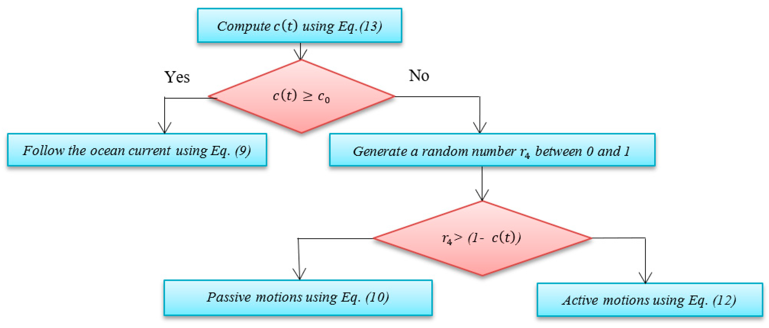
Figure 4.
Flowchart of the jellyfish search optimizer (JSO).

Figure 5.
Tuning of the N parameter.

Figure 6.
Comparison between the modified JSO (MJSO) and JSO under the convergence speed.


Figure 7.
Comparison between the measured and estimated data extracted using MJSO on SDM for R.T.C France.
Figure 7.
Comparison between the measured and estimated data extracted using MJSO on SDM for R.T.C France.

Figure 8.
Comparison between the measured and estimated data extracted using MJSO on DDM for R.T.C France.
Figure 8.
Comparison between the measured and estimated data extracted using MJSO on DDM for R.T.C France.

Figure 9.
Comparison between the measured and estimated data extracted using MJSO on the PHOTOWATT-PWP201 module.
Figure 9.
Comparison between the measured and estimated data extracted using MJSO on the PHOTOWATT-PWP201 module.

Figure 10.
Comparison of the principal characteristics on the STP6 module.

Figure 11.
Comparison among the algorithms under the convergence speed.

Figure 12.
Depiction of the principal characteristics on SM55 module at varied temperatures.

Figure 13.
Depiction of error value between all I measured and estimated data on SDM for the SM55 module at different T and G = 1000.
Figure 13.
Depiction of error value between all I measured and estimated data on SDM for the SM55 module at different T and G = 1000.

Figure 14.
Depiction of the principal characteristics on SM55 module.

Figure 15.
Depiction of error value between all I measured and estimated data on SDM for SM55 module at different irradiance.
Figure 15.
Depiction of error value between all I measured and estimated data on SDM for SM55 module at different irradiance.


Figure 16.
Depiction of the principal characteristics on ST40 module.

Figure 17.
Depiction of error value between all I measured and estimated data on SDM for the ST40 module at different irradiance.
Figure 17.
Depiction of error value between all I measured and estimated data on SDM for the ST40 module at different irradiance.


Figure 18.
Depiction of the principal characteristics on the ST40 module at G = 1000.

Figure 19.
Depiction of error value between all I measured and estimated data on SDM on ST40 module at different T and G = 1000.
Figure 19.
Depiction of error value between all I measured and estimated data on SDM on ST40 module at different T and G = 1000.

Figure 20.
Convergence curve obtained on the ST40 based on SDM under different G and T.

Figure 21.
Depiction of the measured and simulated data obtained by MJSO on SM55 under different T.

Figure 22.
Depiction of error value between all I measured and estimated data on the SM55 module at different T and G = 1000.
Figure 22.
Depiction of error value between all I measured and estimated data on the SM55 module at different T and G = 1000.

Figure 23.
Depiction of the estimated and measured data obtained by MJSO on SM55 under different G with T = 25 °C.
Figure 23.
Depiction of the estimated and measured data obtained by MJSO on SM55 under different G with T = 25 °C.

Figure 24.
Depiction of error value between all I measured and estimated data on the SM55 module at different irradiance.
Figure 24.
Depiction of error value between all I measured and estimated data on the SM55 module at different irradiance.

Figure 25.
Depiction of the measured and simulated data obtained by MJSO on ST40 under different G with T = 25 °C.
Figure 25.
Depiction of the measured and simulated data obtained by MJSO on ST40 under different G with T = 25 °C.

Figure 26.
Depiction of error value between all I measured and estimated data on the ST40 module at different irradiance.
Figure 26.
Depiction of error value between all I measured and estimated data on the ST40 module at different irradiance.

Figure 27.
Depiction of the measured and simulated data on the ST40 module under G = 1000 W/m2 with four different temperature levels.
Figure 27.
Depiction of the measured and simulated data on the ST40 module under G = 1000 W/m2 with four different temperature levels.

Figure 28.
Depiction of error value between all I measured and estimated data on the ST40 module at different T and G = 1000.
Figure 28.
Depiction of error value between all I measured and estimated data on the ST40 module at different T and G = 1000.

Figure 29.
Convergence curve under different operating conditions.


Table 1.
Depiction of an initial solution for SDM.
| 0.760775 | 3.23E-07 | 0.036377 | 53.718523 | 1.481183 |
Table 2.
Depiction of an initial solution for DDM.
| 0.76077 | 2.7E-07 | 0.036561 | 54.5337 | 1.8266 | 2.49E-07 | 1.4609 |
Table 3.
The search boundaries of each unknown parameter.
| Parameter | R.T.C. France Cell | Photowatt-PWP201 | STP6-120/36 | |||
|---|---|---|---|---|---|---|
| (A) | 0 | 1 | 0 | 2 | 0 | 8 |
| , , (A) | 0 | 1E-06 | 0 | 50E-06 | 0 | 50E-06 |
| (Ω) | 0 | 0.5 | 0 | 2 | 0 | 0.36 |
| (Ω) | 0 | 100 | 0 | 2000 | 0 | 1500 |
| , , | 1 | 2 | 1 | 50 | 1 | 50 |
Table 4.
Upper bound and lower bound for unknown parameters of both SM55 and ST40.
| Parameter | SM55 and ST40 | |
|---|---|---|
| (A) | 0 | 2* |
| 0 | 100E-06 | |
| (Ω) | 0 | 2 |
| (Ω) | 0 | 5000 |
| , , /cell | 1 | 4 |
Table 5.
Parameter settings of the compared algorithms.
| Algorithm | Parameter | Value | Algorithm | Parameter | Value |
|---|---|---|---|---|---|
| CPMPSO | N | 50 | MJSO | N | 17 |
| (Number of evaluations) | 80,000 | 50,000 | |||
| Acceleration coefficient () | 1.49445 | 3 | |||
| Acceleration coefficient () | 1.49445 | 0.5 | |||
| Inertia weight (w) | 0.7298 | ||||
| ITLBO | N | 50 | JSO | N | 50 |
| 80,000 | 80,000 | ||||
| WOA | N | 50 | GNDO | N | 50 |
| 80,000 | 80,000 | ||||
| 1 | |||||
| SCA | N | 50 | |||
| 80,000 |
Table 6.
Comparison of the R.T.C. France SDM based on the best-extracted parameter values and their RMSE.
Table 6.
Comparison of the R.T.C. France SDM based on the best-extracted parameter values and their RMSE.
| Algorithms | RMSE | |||||
|---|---|---|---|---|---|---|
| ITLBO [48] | 0.760788 | 3.11E-07 | 0.036547 | 52.88979 | 1.477268 | 0.0007730063 |
| JSO [40] | 0.76079 | 3.11E-07 | 0.036547 | 52.888226 | 1.477272 | 0.0007730063 |
| CPMPSO [46] | 0.760788 | 3.11E-07 | 0.036547 | 52.88979 | 1.477268 | 0.0007730063 |
| WOA [60] | 0.761629 | 3.86E-07 | 0.035308 | 45.93082 | 1.499535 | 0.0010858206 |
| SCA [50] | 0.75826 | 4.09E-07 | 0.035951 | 68.838809 | 1.505000 | 0.0024834154 |
| GNDO [22] | 0.760788 | 3.11E-07 | 0.036547 | 52.88979 | 1.477268 | 0.0007730063 |
| MJSO | 0.760788 | 3.11E-07 | 0.036547 | 52.88979 | 1.477268 | 0.0007730063 |
Bold values refer to the optimal outcomes.
Table 7.
Comparison of SDM.
| Algorithms | Best | Worst | Avg | SD | Rank | Time (S) |
|---|---|---|---|---|---|---|
| ITLBO [48] | 0.0007730063 | 0.0007730063 | 0.0007730063 | 1.07705E-17 | 1 | 0.62 |
| JSO [40] | 0.0007730063 | 0.0007747280 | 0.0007730737 | 3.12840E-07 | 2 | 0.83 |
| CPMPSO [46] | 0.0007730063 | 0.0007730063 | 0.0007730063 | 9.40000E-18 | 1 | 4.54 |
| WOA [60] | 0.0010858206 | 0.0392926194 | 0.0052829509 | 6.82142E-03 | 4 | 0.63 |
| SCA [50] | 0.0024834154 | 0.0446736790 | 0.0244466994 | 1.50365E-02 | 5 | 0.54 |
| GNDO [22] | 0.0007730063 | 0.0007730063 | 0.0007730063 | 1.04628E-17 | 1 | 1.15 |
| MJSO | 0.0007730063 | 0.0007730063 | 0.0007730063 | 9.76743E-18 | 1 | 0.77 |
Bold values indicate the best results.
Table 8.
Comparison on the DDM in terms of obtained parameter and the corresponding RMSE.
| Algorithms | RMSE | |||||||
|---|---|---|---|---|---|---|---|---|
| ITLBO [48] | 0.7608 | 2.47E-07 | 0.0368 | 53.9599 | 1.4579 | 4.78E-07 | 1.9949 | 0.0007422641 |
| JSO [40] | 0.7608 | 5.38E-07 | 0.0371 | 54.4640 | 1.7980 | 1.61E-07 | 1.4262 | 0.0007541675 |
| CPMPSO [46] | 0.7608 | 7.03E-08 | 0.0378 | 56.2715 | 1.3642 | 1.00E-06 | 1.7963 | 0.0007419371 |
| WOA [60] | 0.7608 | 2.67E-07 | 0.0368 | 51.8538 | 1.4662 | 4.10E-08 | 1.6133 | 0.0007764641 |
| SCA [50] | 0.7684 | 0.00E+00 | 0.0324 | 38.3064 | 1.1740 | 3.84E-07 | 1.4970 | 0.0073511847 |
| GNDO [22] | 0.7608 | 1.00E-06 | 0.0373 | 55.6033 | 1.9051 | 1.40E-07 | 1.4130 | 0.0007423279 |
| MJSO | 0.7608 | 7.03E-08 | 0.0378 | 56.2715 | 1.3642 | 1.00E-06 | 1.7963 | 0.0007419371 |
Bold values indicate the best results.
Table 9.
Comparison of the DDM.
| Algorithms | Rank | Time (S) | ||||
|---|---|---|---|---|---|---|
| ITLBO [48] | 0.0007422641 | 0.0007722457 | 0.0007559007 | 9.86421E-06 | 4 | 0.65 |
| JS [40] | 0.0007541675 | 0.0007841579 | 0.0007703203 | 6.92073E-06 | 5 | 0.99 |
| CPMPSO [46] | 0.0007419371 | 0.0007467838 | 0.0007421432 | 9.08E-07 | 2 | 5.52 |
| WOA [60] | 0.0007764641 | 0.0387099260 | 0.0061785479 | 9.77291E-03 | 7 | 0.65 |
| SCA [50] | 0.0073511847 | 0.0480180357 | 0.0299392021 | 1.61644E-02 | 6 | 0.63 |
| GNDO [22] | 0.0007423279 | 0.0007452253 | 0.0007433514 | 7.17546E-07 | 3 | 1.21 |
| MJSO | 0.0007419371 | 0.0007419406 | 0.0007419372 | 6.39E-10 | 1 | 0.94 |
Bold values indicate the best findings.
Table 10.
Comparison on the Photowatt-PWP201 module under extracted parameter values and the corresponding RMSE.
Table 10.
Comparison on the Photowatt-PWP201 module under extracted parameter values and the corresponding RMSE.
| Algorithms | RMSE | |||||
|---|---|---|---|---|---|---|
| ITLBO [48] | 1.031434 | 2.64E-06 | 1.235634 | 821.6413 | 47.59823 | 0.0020529606 |
| JSO [40] | 1.03137 | 2.64E-06 | 1.235211 | 827.1906 | 47.60654 | 0.0020531476 |
| CPMPSO [46] | 1.031434 | 2.64E-06 | 1.235634 | 821.6413 | 47.59823 | 0.0020529606 |
| WOA [60] | 1.030221 | 4.22E-06 | 1.178008 | 1105.314 | 49.39672 | 0.0022966238 |
| SCA [50] | 1.03364 | 1.18E-05 | 0.930711 | 1268.463 | 53.72168 | 0.0117780330 |
| GNDO [22] | 1.031434 | 2.64E-06 | 1.235634 | 821.6413 | 47.59823 | 0.0020529606 |
| MJSO | 1.031434 | 2.64E-06 | 1.235634 | 821.6413 | 47.59823 | 0.0020529606 |
Bold values refer to the optimal results.
Table 11.
Comparison on the Photowatt-PWP201 module.
| Algorithms | Rank | Time (S) | ||||
|---|---|---|---|---|---|---|
| ITLBO [48] | 0.0020529606 | 0.0020529606 | 0.0020529606 | 8.60342E-18 | 1 | 0.57 |
| JSO [40] | 0.0020531476 | 0.0020721180 | 0.0020582422 | 5.22985E-06 | 2 | 0.85 |
| CPMPSO [46] | 0.0020529606 | 0.0020529606 | 0.0020529606 | 7.59000E-18 | 1 | 4.94 |
| WOA [60] | 0.0022966238 | 0.2742508362 | 0.0733819237 | 9.48170E-02 | 4 | 0.53 |
| SCA [50] | 0.0117780330 | 0.2743100751 | 0.1712452167 | 1.20550E-01 | 5 | 0.52 |
| GNDO [22] | 0.0020529606 | 0.0020529606 | 0.0020529606 | 2.04091E-17 | 1 | 1.20 |
| MJSO | 0.0020529606 | 0.0020529606 | 0.0020529606 | 1.05495E-17 | 1 | 0.82 |
Bold values indicate the optimal outcomes.
Table 12.
Comparison on the STP6-120/36 in terms of extracted parameter and the corresponding RMSE.
| Algorithms | RMSE | |||||
|---|---|---|---|---|---|---|
| ITLBO [48] | 7.475284 | 1.93E-06 | 0.168918 | 570.1972 | 44.80042 | 0.0142510636 |
| JSO [40] | 7.47525 | 1.93E-06 | 0.168905 | 571.5660 | 44.80254 | 0.0142510668 |
| CPMPSO [46] | 7.475284 | 1.93E-06 | 0.168918 | 570.1975 | 44.80042 | 0.0142510636 |
| WOA [60] | 7.503181 | 3.27E-06 | 0.157818 | 307.7831 | 46.40846 | 0.0175819626 |
| SCA [50] | 7.56027 | 1.70E-06 | 0.173188 | 323.9495 | 44.38346 | 0.0524438250 |
| GNDO [22] | 7.475284 | 1.93E-06 | 0.168918 | 570.1972 | 44.80042 | 0.0142510636 |
| MJSO | 7.475284 | 1.93E-06 | 0.168918 | 570.1975 | 44.80042 | 0.0142510636 |
Bold values refer to the optimal findings.
Table 13.
Comparison of the STP6-120/36 module.
| Algorithms | Rank | Time (S) | ||||
|---|---|---|---|---|---|---|
| ITLBO [48] | 0.0142510636 | 0.0142510636 | 0.0142510636 | 6.48898E-17 | 1 | 0.59 |
| JSO [40] | 0.0142510668 | 0.0142787559 | 0.0142541538 | 5.09788E-06 | 2 | 0.89 |
| CPMPSO [46] | 0.0142510636 | 0.0142510636 | 0.0142510636 | 6.43E-17 | 1 | 4.2 |
| WOA [60] | 0.0175819626 | 1.4131220500 | 0.3060754580 | 4.56106E-01 | 3 | 0.54 |
| SCA [50] | 0.0524438250 | 1.4131220567 | 0.4211660060 | 5.09904E-01 | 4 | 0.61 |
| GNDO [22] | 0.0142510636 | 0.0142510636 | 0.0142510636 | 4.99530E-17 | 1 | 1.18 |
| MJSO | 0.0142510636 | 0.0142510636 | 0.0142510636 | 5.54223E-17 | 1 | 0.84 |
Bold values indicate the best results.
Table 14.
Comparison at T = 25 °C and various G.
| Algorithm | ST40 | SM55 | ||||||
|---|---|---|---|---|---|---|---|---|
| Avg | Worst | Best | SD | Avg | Worst | Best | SD | |
| G = 1000 W/m2 | ||||||||
| ITLBO [48] | 0.0005639798 | 0.0005639798 | 0.0005639798 | 1.56E-17 | 0.0010291774 | 0.0010291774 | 0.001029177 | 2.69E-17 |
| GNDO [22] | 0.0005639798 | 0.0005639798 | 0.0005639798 | 1.63E-17 | 0.0010291774 | 0.0010291774 | 0.001029177 | 2.42E-17 |
| MJSO | 0.0005639798 | 0.0005639798 | 0.0005639798 | 1.93E-17 | 0.0010291774 | 0.0010291774 | 0.001029177 | 2.14E-17 |
| G = 800 W/m2 | ||||||||
| ITLBO [48] | 0.0005922938 | 0.0005922938 | 0.0005922938 | 1.17E-17 | 0.0005894903 | 0.0005894903 | 0.00058949 | 2.28E-17 |
| GNDO [22] | 0.0005922938 | 0.0005922938 | 0.0005922938 | 1.44E-17 | 0.0005894903 | 0.0005894903 | 0.00058949 | 2.07E-17 |
| MJSO | 0.0005922938 | 0.0005922938 | 0.0005922938 | 1.34E-17 | 0.0005894903 | 0.0005894903 | 0.00058949 | 2.33E-17 |
| G = 600 W/m2 | ||||||||
| ITLBO [48] | 0.0005846744 | 0.0005846744 | 0.0005846744 | 7.94E-18 | 0.0007395954 | 0.0007395954 | 0.000739595 | 1.60E-17 |
| GNDO [22] | 0.0005846744 | 0.0005846744 | 0.0005846744 | 9.50E-18 | 0.0007395954 | 0.0007395954 | 0.000739595 | 1.92E-17 |
| MJSO | 0.0005846744 | 0.0005846744 | 0.0005846744 | 6.64E-18 | 0.0007395954 | 0.0007395954 | 0.000739595 | 2.11E-17 |
| G = 400 W/m2 | ||||||||
| ITLBO [48] | 0.0005617498 | 0.0005617498 | 0.0005617498 | 9.22E-18 | 0.0007047463 | 0.0007047463 | 0.000704746 | 2.28E-17 |
| GNDO [22] | 0.0005617498 | 0.0005617498 | 0.0005617498 | 9.91E-18 | 0.0007047463 | 0.0007047463 | 0.000704746 | 2.07E-17 |
| MJSO | 0.0005617498 | 0.0005617498 | 0.0005617498 | 8.87E-18 | 0.0007047463 | 0.0007047463 | 0.000704746 | 2.33E-17 |
| G = 200 W/m2 | ||||||||
| ITLBO [48] | 0.0004637921 | 0.0004637921 | 0.0004637921 | 1.98E-18 | 0.0003198549 | 0.0003198549 | 0.000319855 | 2.69E-17 |
| GNDO [22] | 0.0004637921 | 0.0004637921 | 0.0004637921 | 2.61E-18 | 0.0003198549 | 0.0003198549 | 0.000319855 | 2.42E-17 |
| MJSO | 0.0004637921 | 0.0004637921 | 0.0004637921 | 2.70E-18 | 0.0003198549 | 0.0003198549 | 0.000319855 | 2.14E-17 |
Bold values indicate the best results.
Table 15.
Comparison at various T and G = 1000 W/m2.
| Algorithm | ST40 | SM55 | ||||||
|---|---|---|---|---|---|---|---|---|
| Avg | Worst | Best | SD | Best | Avg | Worst | SD | |
| T = 25 °C | T = 25 °C | |||||||
| ITLBO [48] | 0.000564 | 0.000564 | 0.000564 | 1.33E-17 | 0.0010292 | 0.0010292 | 0.0010292 | 1.92E-17 |
| GNDO [22] | 0.000564 | 0.000564 | 0.000564 | 1.53E-17 | 0.0010292 | 0.0010292 | 0.0010292 | 2.00E-17 |
| MJSO | 0.000564 | 0.000564 | 0.000564 | 1.40E-17 | 0.0010292 | 0.0010292 | 0.0010292 | 2.26E-17 |
| T = 40 °C | T = 40 °C | |||||||
| ITLBO [48] | 0.0007818 | 0.0007818 | 0.0007818 | 1.45E-17 | 0.0026636 | 0.0026636 | 0.0026636 | 3.71E-17 |
| GNDO [22] | 0.0007818 | 0.0007818 | 0.0007818 | 1.75E-17 | 0.0026636 | 0.0026636 | 0.0026636 | 3.54E-17 |
| MJSO | 0.0007818 | 0.0007818 | 0.0007818 | 1.41E-17 | 0.0026636 | 0.0026636 | 0.0026636 | 4.17E-17 |
| T = 55 °C | T = 60 °C | |||||||
| ITLBO [48] | 0.0009651 | 0.0009651 | 0.0009651 | 1.74E-17 | 0.0022478 | 0.0022478 | 0.0022478 | 2.57E-17 |
| GNDO [22] | 0.0009651 | 0.0009651 | 0.0009651 | 2.64E-17 | 0.0022478 | 0.0022478 | 0.0022478 | 4.02E-17 |
| MJSO | 0.0009651 | 0.0009651 | 0.0009651 | 1.03E-17 | 0.0022478 | 0.0022478 | 0.0022478 | 4.87E-17 |
| T = 70 °C | ||||||||
| ITLBO [48] | 0.000539 | 0.000539 | 0.000539 | 1.68E-17 | ||||
| GNDO [22] | 0.000539 | 0.000539 | 0.000539 | 1.67E-17 | ||||
| MJSO | 0.000539 | 0.000539 | 0.000539 | 3.19E-17 | ||||
Bold values indicate the best results.
Table 16.
The estimated parameters by MJSO at various G and T levels based on SDM.
| Parameter | ST40 | SM55 | Parameter | ST40 | SM55 |
|---|---|---|---|---|---|
| T = 25 °C, and G = 200 W/m2 | T = 40 °C, and G = 1000 W/m2 | ||||
| (A) | 0.53312 | 0.691509545 | (A) | 2.68115 | 3.469926504 |
| (A) | 1.45E-06 | 1.46E-07 | (A) | 5.49E-06 | 9.68E-07 |
| () | 1.17734 | 0.286523008 | () | 1.13189 | 0.320563643 |
| () | 345.15083 | 448.2175783 | () | 359.65270 | 495.0786498 |
| 1.49906 | 1.183446863 | 1.47289 | 1.20188218 | ||
| RMSE | 0.00046379 | 0.000319855 | RMSE | 0.0007818 | 0.002663588 |
| T = 25 °C, and G = 400 W/m2 | T = 55 °C, and G = 1000 W/m2 | ||||
| (A) | 1.06765 | 1.382832492 | (A) | 2.6911303 | |
| (A) | 1.76E-06 | 1.01E-07 | (A) | 2.07E-05 | |
| () | 1.09107 | 0.39516802 | () | 1.13961 | |
| () | 360.63189 | 427.3227638 | () | 306.99020 | |
| 1.51885 | 1.159532356 | 1.46206 | |||
| RMSE | 0.00056175 | 0.000704746 | RMSE | 0.000965 | |
| T = 25 °C, and G = 600 W/m2 | G = 1000 W/m2, and T = 60 °C | ||||
| (A) | 1.60485 | 2.07096087 | (A) | 3.495231764 | |
| (A) | 1.42E-06 | 1.51E-07 | (A) | 6.28E-06 | |
| () | 1.11530 | 0.332953565 | () | 0.323433045 | |
| () | 346.98896 | 447.9630777 | () | 456.4139753 | |
| 1.49405 | 1.187025834 | 1.195804351 | |||
| RMSE | 0.0005847 | 0.000739595 | RMSE | 0.002247768 | |
| T = 25 °C and G = 800 W/m2 and T = 25 °C | T = 70 °C, and G = 1000 W/m2 | ||||
| (A) | 2.13808 | 2.760435313 | (A) | 2.692803 | |
| (A) | 1.14E-06 | 1.41E-07 | (A) | 8.41E-05 | |
| () | 1.12708 | 0.339101259 | () | 1.12991 | |
| () | 332.00526 | 458.1129235 | () | 356.24166 | - |
| 1.47140 | 1.182239275 | 1.47490 | |||
| RMSE | 0.0005923 | 0.00058949 | RMSE | 0.0005390 | |
| T = 25 °C and G = 1000 W/m2 | |||||
| (A) | 2.67589 | 3.45018412 | |||
| (A) | 1.5005E-06 | 1.67E-07 | |||
| () | 1.11484 | 0.330128968 | |||
| () | 356.13413 | 480.8300872 | |||
| 1.49837 | 1.194667673 | ||||
| RMSE | 0.00056 | 0.001029177 | |||
Table 17.
Comparison at T = 25 °C and at various G.
| Algorithm | ST40 | SM55 | ||||||
|---|---|---|---|---|---|---|---|---|
| Best | Avg. | Worst | SD | Best | Avg. | Worst | SD | |
| G = 200 W/m2 | ||||||||
| ITLBO [48] | 0.0004415083 | 0.0004497670 | 0.0004978335 | 1.07E-05 | 0.0003198549 | 0.0003285538 | 0.0005203898 | 3.72E-05 |
| GNDO [22] | 0.0004412887 | 0.0004561559 | 0.0004602882 | 7.63E-06 | 0.0003198549 | 0.0003198549 | 0.0003198549 | 2.05E-18 |
| MJSO | 0.0004411123 | 0.0004453019 | 0.0004602866 | 7.67E-06 | 0.0003198549 | 0.0003198549 | 0.0003198549 | 1.61E-18 |
| G = 400 W/m2 | ||||||||
| ITLBO [48] | 0.0005617498 | 0.0005617498 | 0.0005617498 | 5.66E-18 | 0.0007047463 | 0.0007047463 | 0.0007047463 | 3.67E-18 |
| GNDO [22] | 0.0005617498 | 0.0005617498 | 0.0005617498 | 1.06E-17 | 0.0007047463 | 0.0007047463 | 0.0007047463 | 4.41E-18 |
| MJSO | 0.0005617498 | 0.0005617498 | 0.0005617498 | 8.94E-18 | 0.0007047463 | 0.0007047463 | 0.0007047463 | 5.77E-18 |
| G = 600 W/m2 | ||||||||
| ITLBO [48] | 0.0005846744 | 0.0005916726 | 0.0006381399 | 1.07E-05 | 0.0007395954 | 0.0007550137 | 0.0008904002 | 3.77E-05 |
| GNDO [22] | 0.0005846744 | 0.0005846943 | 0.0005850305 | 7.73E-08 | 0.0007395954 | 0.0007395954 | 0.0007395954 | 1.72E-17 |
| MJSO | 0.0005846744 | 0.0005846744 | 0.0005846744 | 1.52E-17 | 0.0007395954 | 0.0007395954 | 0.0007395954 | 3.09E-17 |
| G = 800 W/m2 | ||||||||
| ITLBO [48] | 0.0005922938 | 0.0006535996 | 0.0012032795 | 1.36E-04 | 0.0005894903 | 0.0007796570 | 0.0058091595 | 0.000951 |
| GNDO [22] | 0.0005922938 | 0.0005937060 | 0.0006330156 | 7.43E-06 | 0.0005894903 | 0.0005894903 | 0.0005894903 | 2.36E-17 |
| MJSO | 0.0005922938 | 0.0005922938 | 0.0005922938 | 1.51E-17 | 0.0005894903 | 0.0005894903 | 0.0005894903 | 2.81E-17 |
| G = 1000 W/m2 | ||||||||
| ITLBO [48] | 0.0005639798 | 0.0006215359 | 0.0010948758 | 1.13E-04 | 0.0010291774 | 0.0010570765 | 0.0012518618 | 5.89E-05 |
| GNDO [22] | 0.0005639798 | 0.0005643865 | 0.0005721906 | 1.54E-06 | 0.0010291774 | 0.0010291774 | 0.0010291774 | 1.90E-17 |
| MJSO | 0.0005639798 | 0.0005639798 | 0.0005639798 | 2.42E-17 | 0.0010291774 | 0.0010291774 | 0.0010291774 | 3.28E-17 |
Bold value refers to the best result.
Table 18.
Comparison among Improved Teaching Learning-Based Optimization (ITLBO), generalized normal distribution optimization (GNDO), and MJSO at G = 1000 W/m2 and various T.
Table 18.
Comparison among Improved Teaching Learning-Based Optimization (ITLBO), generalized normal distribution optimization (GNDO), and MJSO at G = 1000 W/m2 and various T.
| Algorithm | ST40 | SM55 | ||||||
|---|---|---|---|---|---|---|---|---|
| Best | Avg. | Worst | SD | Best | Avg. | Worst | SD | |
| T = 25 °C | T = 25 °C | |||||||
| ITLBO [48] | 0.0005639798 | 0.0005975313 | 0.0007920238 | 5.44E-05 | 0.0010291774 | 0.0010792842 | 0.0013427016 | 9.85E-05 |
| GNDO [22] | 0.0005639798 | 0.0005644851 | 0.0005707906 | 1.63E-06 | 0.0010291774 | 0.0010291774 | 0.0010291774 | 2.00E-17 |
| MJSO | 0.0005639798 | 0.0005639804 | 0.0005639971 | 3.16E-09 | 0.0010291774 | 0.0010291774 | 0.0010291774 | 3.22E-17 |
| T = 40 °C | T = 40 °C | |||||||
| ITLBO [48] | 0.0007818401 | 0.0008411024 | 0.0012483674 | 1.11E-04 | 0.0026635883 | 0.0026698511 | 0.0027624654 | 2.15E-05 |
| GNDO [22] | 0.0007818401 | 0.0007818738 | 0.0007824605 | 1.27E-07 | 0.0026635883 | 0.0026635883 | 0.0026635883 | 5.21E-17 |
| MJSO | 0.0007818401 | 0.0007818401 | 0.0007818401 | 2.72E-17 | 0.0026635883 | 0.0026635883 | 0.0026635883 | 8.00E-17 |
| T = 55 °C | T = 60 °C | |||||||
| ITLBO [48] | 0.0008751784 | 0.0009265589 | 0.0009647880 | 3.31E-05 | 0.0022477676 | 0.0023141713 | 0.0030494582 | 0.000153 |
| GNDO [22] | 0.0008845343 | 0.0009462633 | 0.0009636183 | 3.20E-05 | 0.0022477676 | 0.0022478880 | 0.0022495080 | 3.85E-07 |
| MJSO | 0.0008751733 | 0.0009252746 | 0.0009636183 | 4.19E-05 | 0.0022477676 | 0.0022477676 | 0.0022477676 | 7.72E-17 |
| T = 70 °C | ||||||||
| ITLBO [48] | 0.0005390036 | 0.0005409504 | 0.0005711203 | 6.55E-06 | ||||
| GNDO [22] | 0.0005390036 | 0.0005390036 | 0.0005390036 | 1.02E-16 | ||||
| MJSO | 0.0005390036 | 0.0005390036 | 0.0005390036 | 2.87E-17 | ||||
Bold value indicates the best result.
Table 19.
The estimated parameters by MJSO at various G and T levels based on DDM.
| Parameter | ST40 | SM55 | Parameter | ST40 | SM55 |
|---|---|---|---|---|---|
| T = 25 °C and G = 200 W/m2 | G = 1000 W/m2 and T = 40 °C | ||||
| (A) | 0.533128071 | 0.691509545 | (A) | 2.681147085 | 3.469926503 |
| (A) | 1.00E-04 | 1.46E-07 | (A) | 5.49E-06 | 9.68E-07 |
| () | 1.389590565 | 0.286522984 | () | 1.131889775 | 0.320563644 |
| () | 361.5945492 | 448.2175819 | () | 359.6526938 | 495.0786584 |
| 3.695395541 | 1.183446871 | 1.47288933 | 1.201882177 | ||
| (A) | 6.63E-07 | 4.36E-10 | (A) | 4.79E-16 | 2.67E-20 |
| 1.415993437 | 1.183446104 | 3.894289586 | 1.059268814 | ||
| RMSE | 0.000441112 | 0.000319855 | RMSE | 0.00078184 | 0.002663588 |
| T = 25 °C and G = 400 W/m2 | T = 55 °C and G = 1000 W/m2 | ||||
| (A) | 1.067647486 | 1.382832493 | (A) | 2.691114387 | |
| (A) | 1.76E-06 | 1.01E-07 | (A) | 2.02E-05 | |
| () | 1.091071212 | 0.395168019 | () | 1.139967319 | |
| () | 360.6318995 | 427.322756 | () | 307.4107912 | |
| 1.518853785 | 1.159532355 | 1.460050927 | |||
| (A) | 5.89E-07 | 7.66E-07 | (A) | 1.00E-06 | |
| 1.198084303 | 2.811330228 | 1.803428118 | |||
| RMSE | 0.00056175 | 0.000704746 | RMSE | 0.000963618 | |
| T = 25 °C and G = 600 W/m2 | G = 1000 W/m2 and T = 60 °C | ||||
| (A) | 1.604854997 | 2.07096087 | (A) | 3.495231762 | |
| (A) | 4.18E-07 | 2.99E-19 | (A) | 6.28E-06 | |
| () | 1.115301286 | 0.332953561 | () | 0.323433041 | |
| () | 346.9889634 | 447.9630754 | () | 456.4140324 | |
| 1.494046019 | 1.530239528 | 1.195804357 | |||
| (A) | 1.00E-06 | 1.51E-07 | (A) | 4.96E-18 | |
| 1.494046072 | 1.187025838 | 1.143884255 | |||
| RMSE | 0.000584674 | 0.000739595 | RMSE | 0.002247768 | |
| T = 25 °C and G = 800 W/m2 | G = 1000 W/m2 and T = 70 °C | ||||
| (A) | 2.138075668 | 2.760435313 | (A) | 2.675888717 | |
| (A) | 4.78E-07 | 1.00E-17 | (A) | 1.50E-06 | |
| () | 1.127075246 | 0.339101255 | () | 1.114835111 | |
| () | 332.0052634 | 458.1129287 | () | 356.1341223 | - |
| 1.471397046 | 3.966370682 | 1.498371345 | |||
| (A) | 6.60E-07 | 1.41E-07 | (A) | 4.38E-20 | |
| 1.47139699 | 1.182239278 | 1.291342175 | |||
| RMSE | 0.000592294 | 0.00058949 | RMSE | 0.00056398 | |
| T = 25 °C and G = 1000 W/m2 | |||||
| (A) | 2.675888718 | 3.45018412 | |||
| (A) | 1.50E-06 | 2.72E-20 | |||
| () | 1.114835118 | 0.330128971 | |||
| () | 356.134117 | 480.8300837 | |||
| 1.498371336 | 1.558723379 | ||||
| (A) | 2.34E-19 | 1.67E-07 | |||
| 1.355469966 | 1.194667667 | ||||
| RMSE | 0.00056398 | 0.001029177 | |||
Publisher’s Note: MDPI stays neutral with regard to jurisdictional claims in published maps and institutional affiliations. |
© 2021 by the authors. Licensee MDPI, Basel, Switzerland. This article is an open access article distributed under the terms and conditions of the Creative Commons Attribution (CC BY) license (http://creativecommons.org/licenses/by/4.0/).
Share and Cite
MDPI and ACS Style
Abdel-Basset, M.; Mohamed, R.; Chakrabortty, R.K.; Ryan, M.J.; El-Fergany, A. An Improved Artificial Jellyfish Search Optimizer for Parameter Identification of Photovoltaic Models. Energies 2021, 14, 1867. https://doi.org/10.3390/en14071867
AMA Style
Abdel-Basset M, Mohamed R, Chakrabortty RK, Ryan MJ, El-Fergany A. An Improved Artificial Jellyfish Search Optimizer for Parameter Identification of Photovoltaic Models. Energies. 2021; 14(7):1867. https://doi.org/10.3390/en14071867
Chicago/Turabian StyleAbdel-Basset, Mohamed, Reda Mohamed, Ripon K. Chakrabortty, Michael J. Ryan, and Attia El-Fergany. 2021. "An Improved Artificial Jellyfish Search Optimizer for Parameter Identification of Photovoltaic Models" Energies 14, no. 7: 1867. https://doi.org/10.3390/en14071867
Note that from the first issue of 2016, this journal uses article numbers instead of page numbers. See further details here.