Calibration and Validation of ArcGIS Solar Radiation Tool for Photovoltaic Potential Determination in the Netherlands

Abstract

Geographic information system (GIS) based tools have become popular for solar photovoltaic (PV) potential estimations, especially in urban areas. There are readily available tools for the mapping and estimation of solar irradiation that give results with the click of a button. Although these tools capture the complexities of the urban environment, they often miss the more important atmospheric parameters that determine the irradiation and potential estimations. Therefore, validation of these models is necessary for accurate potential energy yield and capacity estimations. This paper demonstrates the calibration and validation of the solar radiation model developed by Fu and Rich, employed within ArcGIS, with a focus on the input atmospheric parameters, diffusivity and transmissivity for the Netherlands. In addition, factors affecting the model’s performance with respect to the resolution of the input data were studied. Data were calibrated using ground measurements from Royal Netherlands Meteorological Institute (KNMI) stations in the Netherlands and validated with the station data from Cabauw. The results show that the default model values of diffusivity and transmissivity lead to substantial underestimation or overestimation of solar insolation. In addition, this paper also shows that calibration can be performed at different time scales depending on the purpose and spatial resolution of the input data.

1. Introduction

Geographic Information System (GIS) based solar photovoltaic (PV) tools have been developed and used increasingly in the past decade, as they provide a remote assessment of PV siting, planning, integration and management [1]. These tools have been gaining popularity within the public sector (general public, governments, etc.) and also the private sector (PV installers, network operators, etc.). With increasing interest in sustainable solar energy generation, the mapping of solar PV potential has been explored by many at local [2,3], municipal [4,5] and regional scales [6]. At a local scale, it is easy and insightful to assess individual buildings. This information, once generated, can be used for answering several questions regarding the planning and siting of solar PV or solar thermal systems and even in urban planning and policy evaluations [7,8].

Early methods for PV potential calculations used computational solar radiation models which were either top-down or could not capture complex roof tops or probable shading due to the surroundings [9,10]. Then, a combination of computational models and GIS methods emerged for improving the solar irradiance calculations and for the estimation of technical [6,11,12,13] and socio-economic potential [14]. GIS based algorithms, on the other hand, help in capturing the spatio-temporal variation of solar irradiation and, consequently, PV yields [15]. A number of solar irradiation and PV mapping tools that are currently available and use different methodologies for rooftop PV potential analyses have been reviewed [16,17,18]. These algorithms are driven by geographic data and atmospheric parameters specific to the particular area. Most of the GIS based methods are based on some form of geographic data, such as satellite images, digital elevation models (DEM) [10,14,17] or LiDAR data [19,20,21,22]. These methods use different assumptions and, hence, differ in their accuracy and performance. Usually, the most common assumption is that every point on the rooftop receives an equal amount of solar radiation, irrespective of the slope, orientation and shading factors. Such assumptions often lead to inaccuracies [23]. When it comes to preparing maps or creating PV potential tools, it is necessary that the tool is customized to suit the geographic area, as solar irradiation and its associated weather parameters change drastically depending on the location and time. Commonly used solar irradiance models have been reviewed and analyzed [9,10,18]. Out of the few existing raster-based models, the GRASS r.sun model developed by Šúri and Hofierka [24] and ESRI’s Solar Radiation used in ArcGIS [25], developed by Fu and Rich [26], allow for integration of attributes that vary spatially over large regions. In addition, these models also account for shadows from surrounding buildings and trees, while allowing modeling over inclined surfaces, which is of specific interest in the urban landscape.

For solar irradiance calculations, GRASS r.sun uses a Linke turbidity factor and beam and diffuse radiation coefficients, which are obtained from a data bank and calculated from decomposing global radiation measurements from a nearby weather station [27]. On the other hand, ArcGIS’s Solar Radiation uses simplified models, in addition to an easily operable interface with high resolution geospatial graphics. In addition, in the Solar Radiation tool, sky transmissivity and diffusivity parameters for calculation of direct and diffuse insolation are values which can be changed via a time series; throughout the year, every month, or within a day. Diffusivity ranges from zero to one, with typical values of 0.2–0.3 for clear sky conditions. Transmissivity also ranges from zero to one, with 0.5–0.7 for clear skies. Note that transmissivity and diffusivity are inversely related [28]. The GRASS r.sun is an opensource software, while ESRI’s Solar Radiation is a proprietary software.

The atmospheric parameters (Linke turbidity factor, clear-sky index, transmissivity, etc.) can have a significant impact on the calculated annual irradiation [22,29]. These atmospheric parameters are hard to model and customize for a particular location [24]. Using the tools without validating these variables can have a significant influence on the final results; therefore, using parameters closer to local insolation values reduces the variation in solar radiation estimation [20,30]. Especially, with the Solar Radiation, model validation is necessary since the actual values cannot be defined from atmospheric data prior to model implementation [10]. The Australian PV Institute’s (APVI) Solar Potential Tool, developed by the University of New South Wales, uses the Solar Radiation model as the background [31]. They used validation methods to estimate the accuracy of the APVI tool in comparison to measurements of the output AC power of PV systems and NREL’s System Advisory Model (SAM [32]). The study also analyzed the accuracy of ArcGIS’s Solar Radiation tool with respect to insolation on shaded and unshaded surfaces [33]. Copper and Bruce [31] stated that a linear correction can be applied to ArcGIS’s estimates of insolation in order to achieve better fits with the results from SAM. However, it was observed that studies do not validate these models before using them, despite the influence of this on the results.

This paper, therefore, addresses the relevance and implementation of using calibrated values for diffusivity and transmissivity for estimation of global horizontal irradiation for varying spatial resolutions and geographic areas, using the Solar Radiation tool of ArcGIS, with particular focus on the Netherlands as a case study. We used the typical meteorological year data as well as the most recent 10 years irradiance data for calibration purposes.

This paper is further organized as follows. In Section 2 the methods and data used are presented. Section 3 shows and discusses the results for the annual and monthly analysis of parameters with a validation case. Additionally, the model implemented for varying spatial resolutions is also presented. Section 4 concludes the paper.

2. Materials and Methods

2.1. ArcGIS Solar Radiation Tool

It is evident that solar irradiation varies with time, during a day, in a month and throughout the year. It also varies with the climatic conditions and the position of the sun. Therefore, the challenge for the model is to predict the values as close as possible to reality. The tool is quite simple, requiring only a couple of atmospheric parameters. In the case of the Solar Radiation tool, it is hard to calibrate these atmospheric parameters of diffusivity and transmissivity before running the model. The Solar Radiation tool of ArcGIS’s Spatial Analyst Toolbox calculates the solar radiation over a geographic area or for specified point (latitude–longitude) locations, based on the hemispherical viewshed algorithm explained in [34,35,36]. This tool takes location, elevation, slope, orientation and atmospheric transmission as most the relevant inputs. The total amount of radiation calculated for a given location is given as global radiation in the (energy) units of Wh/m².

The variable parameters we discuss in this paper are atmospheric diffusivity and transmissivity [28], which denote the proportion of global normal radiation flux that is diffuse and the fraction of radiation that passes through the atmosphere (averaged over all wavelengths), respectively. These values, thus, range from 0 to 1. All the calculations were performed under clear sky conditions.

The Solar Radiation tool uses a diffusivity value of 0.3 and transmissivity value of 0.5 as the default settings and this is referred to as the default model throughout this paper. For calibration of the Solar Radiation tool, solar irradiation for all combinations of diffusivity (0.2–0.7) and transmissivity (0.3–0.7) parameters (modelled values) have been simulated. In the results, for the purpose of analysis, these values will be referred to as whole numbers preceded by D or T to denote diffusivity and transmissivity, respectively. For example, D3T5 refers to a diffusivity of 0.3 and transmissivity of 0.5.

2.2. Calibration Data

A major source of meteorological data in the Netherlands comes from the Royal Netherlands Meteorological Institute (KNMI) [37]. This institute provides a wide range of meteorological products and manages 50 automatic ground-based weather stations across the country, of which, 33 stations record the solar irradiance. Calibration of the atmospheric parameters was conducted using the measured values from the KNMI network. The KNMI station at De Bilt, in the Netherlands (52.10N, 5.18E) was chosen as a reference point for data calibration. Irradiation values obtained from the ground stations were mapped and interpolated to identify variations throughout the country for 10 years (2011–2020). The De Bilt station was selected out of the 33 stations that provide irradiation data, as this station is located in the center of the Netherlands and is commonly used as a reference point by KNMI for describing and forecasting the weather in the whole of the Netherlands. In fact, the change in irradiation from coast to mainland is not very prominent (about 10%) [38] and, therefore, a single station (at the center) can well be used as a reference when performing nationwide calculations. The model will be implemented for the area of De Bilt and meteorological data from that station will be used for atmospheric data calibration. For calibration purposes, De Bilt values were chosen in order to see if it was performing adequately to be used for the whole country.

Out of the 33 stations which measure irradiance, 30 stations were selected due to interruptions in the data collection of 3 stations within the 10 years. The locations of these KNMI ground measurement stations and their classification as either coast or mainland used in this study are shown in Figure 1. Daily sums of measured irradiance from the ground stations were gathered and aggregated per month and per year. In addition, irradiation maps for the country were created using a simple inverse distance weighted interpolation technique with irradiation data obtained from these 30 KNMI stations. This provides an insight into the variation in irradiance within the country over the years at low resolution, which is sufficient for checking for anomalies related to localized weather conditions or instrumentation errors [39].

In addition to the KNMI stations, there is a Baseline Surface Radiation Network (BSRN) station at Cabauw in the Netherlands. This is one of the stations that provides radiation measurements as part of a worldwide network [40,41]. There are about 40 stations in this global network in different climatic zones. These data are of primary importance for the validation and evaluation of various satellite and model estimates of radiation parameters. The Netherlands falls under the temperate maritime climate zone and Cabauw (51.97N, 4.93E) is a BSRN station in the Netherlands, which adheres to the highest achievable data measurement standards. Therefore, data from this station were used to validate the calibrated model [42]. This station is about 30 km southwest of De Bilt (see Figure 1).

2.3. Input Data for the Model

Since the Solar Radiation tool is GIS based, it requires inputs in terms of raster or vector data. In particular, the Area Solar Radiation tool requires a DEM as an input to model solar radiation over geographic areas. The DEM used as input in this study is of 50 cm resolution and was obtained from Actueel Hoogtebestand Nederlands (AHN) [43]. Additionally, a DEM of 5 m (AHN) and 30 m (Aster DEM) [44,45] were used for irradiance calculations to evaluate the effect of spatial resolution on the outputs generated. A vector dataset of the locations and attributes of the KNMI and BSRN stations was used to map the measured irradiance values. Spatial resolution is one of the key factors deciding the quality of the output, as can be observed from Figure 2. The higher the resolution, the greater the detail in the images. Therefore, this should be chosen depending on the purpose of use. Modelling irradiation on the rooftops can be performed with 50 cm data, as can be clearly seen from Figure 2c. The slopes and orientations of the rooftops can also be calculated effectively at this resolution, which helps in potential estimations at the building level. With 5 m data, it is likely only possible to do this at the neighborhood or block level. With 30 m data, regional or national level estimations are possible.

2.4. Method

The Solar Radiation model was implemented for calibrating the model parameters T and D. The model has the capability to predict the irradiance values for varying temporal resolutions; daily, monthly, annual average and also within a specified time period. In this paper, the values were calibrated for two cases of varying temporal resolutions; yearly (annual average) and monthly average since this gives better information for potential estimations. In addition to these two temporal scales, we evaluated the data at varying spatial resolutions. All the modelled values were validated against a reference set for the default case, modelled values calibrated per year and modelled values calibrated every month.

The Solar Radiation modeling tool is computationally intensive, the process can run from a few hours up to multiple days depending on the inputs provided. In this particular tool, the simulation time is exponentially proportional to the resolution of the sky size and the raster input [3]. This also means that the higher the resolution of the input image, the greater the detail in the results and longer processing time.

ArcGIS uses Python as a scripting module to perform geographic data analysis, data conversion, data management, and for map automation [46]. Therefore, a customized Python script to run all permutations of atmospheric parameters of the model was incorporated to automatically run and iterate all the combinations of D and T values without manual intervention. The computed values of different permutations and combinations were then calibrated using measured values from the KNMI ground station in De Bilt. The best fit parameters of diffusivity and transmissivity were estimated for each month and year separately. The percentage difference (PD) between measured and modelled values was used to find the best fit values per month and per year (Equation (1)) [47].

Data fitting is highly dependent on the purpose of use, and the spatial and temporal scales at which the result is needed. In this paper, we chose to find the best fit values of global horizontal irradiation (GHI) for one location (De Bilt) over 10 years, assuming that the calibrated values from this location can be used for the whole country. The default model values and the calibrated model values (GHI_mod) were then compared with the measurements from De Bilt (GHI_meas) using percent differences (PD) and mean bias error (MBE). MBE is the statistical model performance indicator, representing the systematic error of the prediction model to under or over estimate. The percentage difference PD and MBE are defined as:

$$\mathrm{PD}=|\left[\left(GH{I}_{meas}-GH{I}_{mod}\right)/GH{I}_{meas}\right]\times 100$$

(1)

$$\mathrm{MBE}=\frac{1}{N}{{\displaystyle \sum }}^{}\left(GH{I}_{mod}-GH{I}_{meas}\right)$$

(2)

with N referring to the number of measurements and the subscripts “meas” and “mod” corresponding to the irradiation values measured at KNMI De Bilt and obtained from the Solar Radiation model for all settings of D and T, respectively. Modelled data are calibrated per month and once a year. Analysis at a local scale to depict buildings was also performed on an area close to the Cabauw station and this was chosen for validating the method.

3. Results and Discussion

This section presents and discusses the results of the calibration and validation methods along with insights into the spatio-temporal variation of solar radiation within the Netherlands. In addition, the purpose of using a GIS based radiation model is presented.

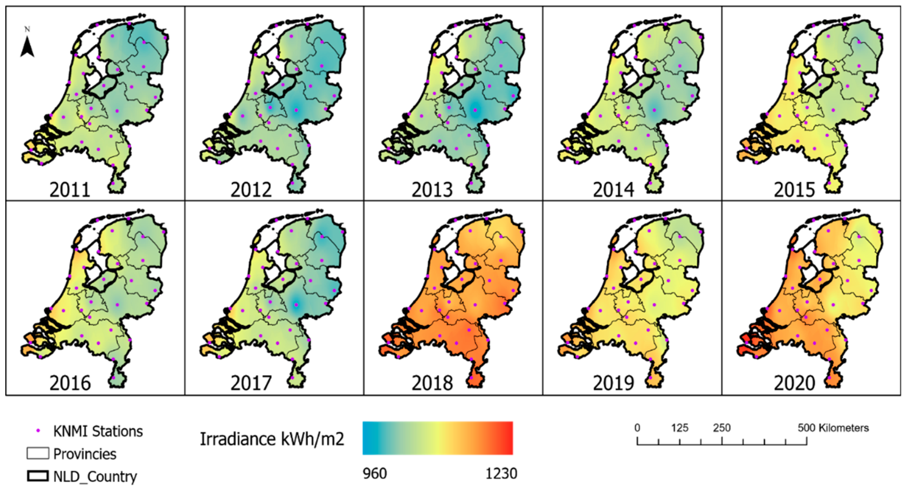
3.1. Spatio-Temporal Variation of Solar Radiation in the Netherlands

Solar irradiation depends on the geographic position and local climatic variations. The spatial and temporal variations in the global solar irradiation in the Netherlands for the years ranging from 2011 till 2020 are shown in Figure 3. The coastal region generally has a higher level of irradiation compared to the mainland. De Bilt, which is in the center of the country, falls in the median zone. Irradiation values from this station can, therefore, be taken as the average for the whole country.

An overview of the ranges of values recorded at the 30 meteorological stations in the Netherlands is shown in Figure 4. The boxplots show the annual irradiation as recorded at the KNMI stations grouped as coast and mainland; 12 stations along the coast and 18 from the mainland (see Figure 1). It is clear that the coastal area has higher irradiation values compared to the mainland. It is worthy to mention that these values are larger than the 30-year average (983.41 kWh/m² measured between 1981–2010) used to characterize the Dutch climate [47]. Extremely high values have been recorded over the past three years.

Table A1. Spatio-temporal variation of measured annual irradiation (kWh/m²) and its standard deviation (std) in the Netherlands, comparing coast, mainland and the central De Bilt location. The coast column contains averaged irradiation values of 12 stations (blue dots in Figure 1) collected over 10 years. Similarly, the mainland irradiation values were obtained from 18 stations away from the coast (red dots in Figure 1).

Year	Annual Irradiation (kWh/m2)
	Coast	std	Mainland	std	De Bilt
30-year average 1	983.41
2011	1067.2	35.4	1042.8	28.8	1026.0
2012	1056.1	30.7	1021.5	21.3	988.7
2013	1070.6	26.5	1020.1	18.6	1003.5
2014	1087.9	19.1	1048.3	24.1	1040.7
2015	1102.4	28.4	1073.9	26.1	1073.2
2016	1105.4	34.5	1053.5	20.4	1039.5
2017	1085.4	30.5	1038.1	29.7	1020.0
2018	1156.9	20.4	1166.4	20.8	1137.2
2019	1119.4	30.8	1100.4	24.7	1098.8
2020	1162.6	28.6	1130.9	33.2	1125.3

¹ Averaged solar radiation from 1981–2010 collected from different KNMI stations [49].

in Appendix A, shows the averaged irradiation values for the coast and mainland categories, collected for the 30 stations in the Netherlands.

From Figure 4, it is also evident that irradiation for location/locations is not the same every year. Even though the spatial variation of irradiation is prominent, even up to some 15% (Figure 3), we choose the De Bilt values for validation of the solar irradiance for the whole country, as this is the central location of the country.

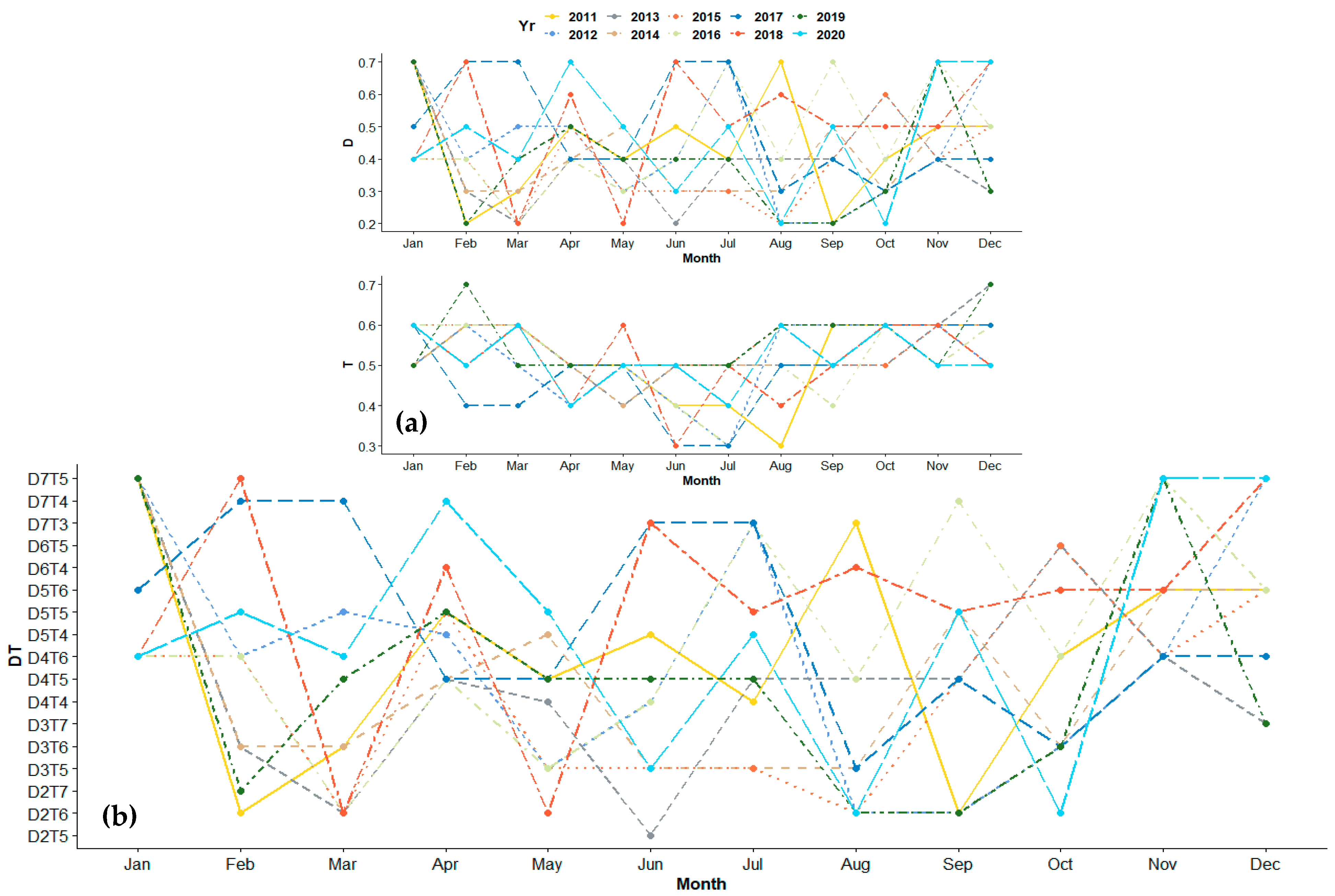
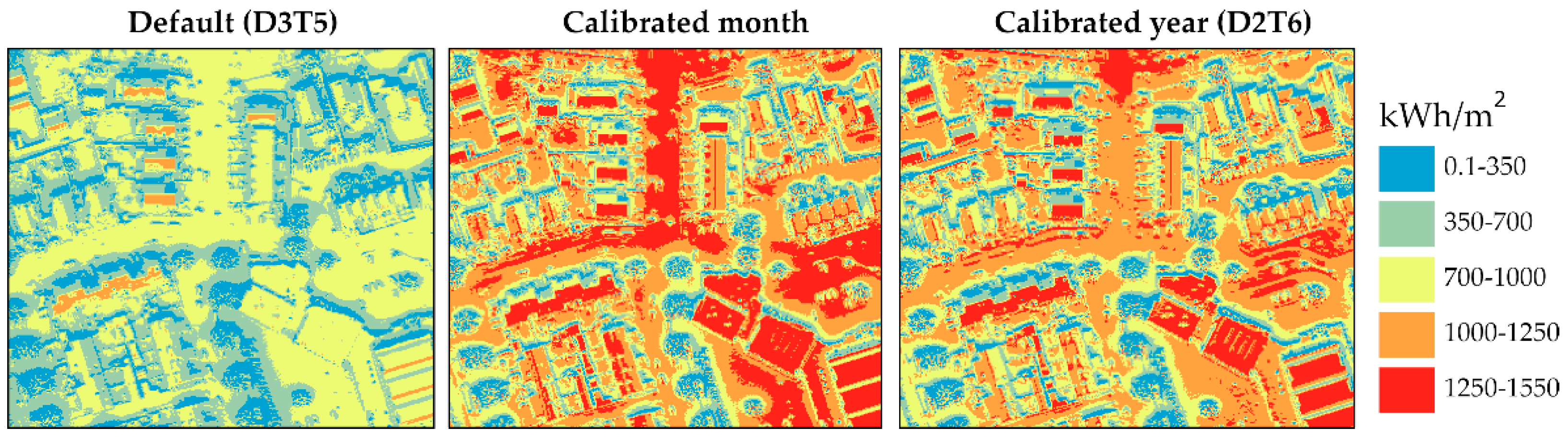
3.2. Calibrated Values vs. Default Values

All combinations of D and T for the 10 years have been modelled for the location of De Bilt.

Table 1. Global horizontal irradiation (GHI) from de Bilt from measured (GHI_meas), results from solar radiation default model D3T5 (GHI_mod) for the year 2020 and the corresponding percentage differences (PD).

Month	GHImeas (kWh/m2)	GHImod (default)	PD (%)	GHI (calibrated)	PD (%)
Jan	16.58	6.94	58.17	17.73	6.93
Feb	31.76	20.33	35.99	30.18	4.98
Mar	93.94	58.73	37.48	100.25	6.73
Apr	155.53	103.23	33.62	151.32	2.70
May	194.33	148.42	23.62	194.94	0.32
Jun	163.95	160.52	2.09	160.52	2.09
Jul	149.01	156.99	5.36	148.31	0.46
Aug	142.56	121.23	14.97	145.79	2.26
Sep	98.51	71.92	26.99	98.96	0.45
Oct	39.66	29.71	25.09	40.66	2.52
Nov	25.90	9.05	65.08	25.96	0.23
Dec	13.53	4.05	70.07	12.53	7.39
Annual	1125.27	891.12	20.81	1090.25	3.11

shows the GHI values measured at the De Bilt station per month for the year 2020 and modelled values from the same location with the default settings and calibrated values (best combinations of D and T) and their corresponding percentage difference (PD). Note, that the modelled values for different years are the same for every combination each month, except for leap years, as shown in

Table A2. Monthly modelled irradiation values for all combination of D and T at de Bilt using Solar Radiation tool.

D	T	Jan	Feb	Mar	Apr	May	Jun	Jul	Aug	Sep	Oct	Nov	Dec
0.2	0.3	0.82	4.30	18.66	40.54	64.27	71.52	68.98	49.54	24.65	7.23	1.25	0.36
0.2	0.4	2.41	9.33	32.85	64.08	96.69	106.06	103.01	76.74	41.75	14.59	3.39	1.23
0.2	0.5	5.67	17.25	51.48	92.25	133.88	145.21	141.82	108.74	63.47	25.48	7.46	3.26
0.2	0.6	11.58	28.88	75.06	125.32	176.08	189.20	185.63	145.79	90.24	40.66	14.45	7.35
0.2	0.7	21.58	45.25	104.31	163.83	223.81	238.59	235.00	188.44	122.73	61.13	25.72	14.92
0.3	0.3	1.00	5.04	21.19	45.19	70.96	78.75	76.06	55.00	27.82	8.39	1.51	0.44
0.3	0.4	2.94	10.97	37.39	71.56	106.96	117.00	113.80	85.37	47.21	16.98	4.10	1.52
0.3	0.5	6.94	20.33	58.73	103.23	148.42	160.52	156.99	121.23	71.92	29.71	9.05	4.05
0.3	0.6	14.22	34.13	85.86	140.58	195.66	209.65	205.99	162.92	102.51	47.55	17.57	9.17
0.3	0.7	26.59	53.68	119.72	184.31	249.41	265.14	261.52	211.20	139.87	71.75	31.40	18.68
0.4	0.3	1.24	6.03	24.58	51.38	79.89	88.38	85.49	62.29	32.04	9.94	1.85	0.56
0.4	0.4	3.66	13.15	43.44	81.53	120.67	131.59	128.18	96.88	54.48	20.15	5.04	1.92
0.4	0.5	8.63	24.44	68.39	117.88	167.80	180.94	177.23	137.87	83.19	35.36	11.16	5.11
0.4	0.6	17.73	41.13	100.25	160.92	221.77	236.92	233.12	185.76	118.88	56.73	21.74	11.60
0.4	0.7	33.27	64.93	140.26	211.62	283.53	300.54	296.87	241.54	162.73	85.90	38.98	23.70
0.5	0.3	1.57	7.42	29.31	60.04	92.38	101.88	98.70	72.49	37.95	12.11	2.34	0.72
0.5	0.4	4.65	16.21	51.92	95.49	139.85	152.02	148.31	113.00	64.66	24.60	6.37	2.47
0.5	0.5	11.00	30.18	81.93	138.37	194.94	209.53	205.55	161.18	98.96	43.25	14.12	6.60
0.5	0.6	22.65	50.94	120.41	189.39	258.32	275.10	271.11	217.74	141.79	69.59	27.57	15.00
0.5	0.7	42.63	80.67	169.01	249.85	331.31	350.09	346.36	284.03	194.73	105.72	49.58	30.73
0.6	0.3	2.07	9.51	36.41	73.04	111.13	122.12	118.51	87.80	46.81	15.36	3.06	0.95
0.6	0.4	6.15	20.80	64.63	116.43	168.62	182.66	178.51	137.17	79.93	31.27	8.36	3.30
0.6	0.5	14.56	38.80	102.23	169.12	235.64	252.42	248.04	196.14	122.62	55.10	18.56	8.82
0.6	0.6	30.03	65.64	150.65	232.10	313.15	332.37	328.10	265.71	176.16	88.87	36.32	20.10
0.6	0.7	56.67	104.28	212.15	307.20	402.97	424.43	420.60	347.75	242.73	135.45	65.50	41.26
0.7	0.3	2.91	12.98	48.25	94.71	142.37	155.85	151.53	113.31	61.58	20.79	4.27	1.35
0.7	0.4	8.64	28.45	85.83	151.32	216.58	233.74	228.85	177.46	105.39	42.39	11.67	4.68
0.7	0.5	20.49	53.17	136.06	220.36	303.49	323.89	318.86	254.41	162.05	74.84	25.96	12.53
0.7	0.6	42.34	90.15	201.04	303.29	404.52	427.81	423.07	345.66	233.45	121.01	50.90	28.60
0.7	0.7	80.07	143.63	284.04	402.78	522.41	548.32	544.33	453.97	322.72	184.99	92.02	58.83

in Appendix A. This is because solar irradiation modelling has been performed on a single location (De Bilt station) with a constant DEM for all the years, assuming that there are no height variations throughout the 10 years. The locations of the ground measurement systems are also usually unchanged and are placed in fields with no obstructions. This clearly indicates that the model is very sensitive to the provided height information, which in turn, can be used in a manner that is dependent on the purpose of the analysis.

From Table 1, it is clear that the default model substantially underestimates the GHI. On an annual basis, for the year 2020, the default model yields an annual sum of 891.12 kWh/m², which is about 21% less than the measured values at De Bilt. Only for two months (June and July) are the percentage differences below 6%, while in the winter months, the differences are much larger. If these values are not adjusted, they might lead to error propagation when these values used in further PV potential estimations. Therefore, it is necessary to find the right combination of D and T parameters in order to achieve better fits and, in turn, better accuracy. Choosing the correct temporal resolution for irradiance estimations is, therefore, important for the final results. For example, when trying to look at the production profile for a single household, hourly irradiance calculations can be very useful, in particular, for optimization of self-consumption. On the other hand, if the purpose is creating an irradiance map for the whole country, then it is more useful to select a seasonal or yearly variation.

The best combination of diffusivity D and transmissivity T values was studied for the Netherlands for every month and for a year as a whole at the De Bilt location. Best fit values for each month were determined by finding the lowest PD between GHI_meas and GHI_mod (Equation (1)). The results for the best combination of D and T and the corresponding error ranges for monthly fits are shown in Figure 5a,b and Figure 6a, respectively.

The difference in PD between the default and the calibrated model is huge (Figure 6a). The PD for the calibrated model is well below 7% for most of the fits. Here, the highest PD was also observed for the winter months, similar to the PD of the default model. Most repeating (four times in 10 years) D and T values are also from the winter months. The variation of best fit D and T values is shown separately for the 10 years in Figure 5a. Figure 6b shows the fits achieved by calibrating the model using the monthly and yearly fits, in comparison with the default model. It is evident as to how much error can be reduced by using calibrated values from Figure 6b. The MBE for the default model for 2020, as shown in Figure 6b, is negative, which means that the model is underestimating the value. Furthermore, analyzing the MBE values for all the 10 years revealed that the default model is biased, which means that for all the 10 years under review, the default model has underestimated the GHI.

Calibrating the values using only one annual DT combination resulted in higher PD values than fitting the data using DT combinations optimized per month, as shown in Table 1. Modelled values, obtained by using one DT combination per year, under estimate the irradiance for winter months and overestimate the irradiance for summer months. Therefore, over a year, the cumulative irradiation values are closer to the reference values. However, the monthly fits are much better when looking at higher temporal scales. On the other hand, if we are looking at lower spatial resolutions (district or country level), yearly fitting could suffice. This is because detailed information would be masked as the DEM input would be coarse (resolution of about 15 m–30 m or larger), which is not enough to distinguish between individual buildings.

To a large extent, yearly fits also reduce the error as compared to the default model, as shown in

Table 2. Best fit DT values on an annual basis and the corresponding PD

Year	DT Year	PD (%)	GHI meas
2011	D4T5	0.78	1026.04
2012	D6T4	0.92	988.75
2013	D6T4	0.56	1003.51
2014	D4T5	2.18	1040.74
2015	D2T6	1.59	1073.18
2016	D4T5	2.07	1039.47
2017	D4T5	0.2	1020.04
2018	D2T6	4.13	1137.19
2019	D2T6	0.78	1098.79
2020	D2T6	3.11	1125.27

. The graph shown in Figure 7, plots the calibrated values of D and T when using one value for the whole year. It can be seen that certain years (2015, 2018–2020) with high levels of radiation have low diffusion and high transmission (D2T6), and low radiation years (2012 and 2013) have high diffusion and low transmission (D6T4), similar to what has been published recently [48]. The rest of the years have a median combination of diffusion and transmission (D4T5). Therefore, on the basis of the trend from these data, and the look up table (Table A2), it is feasible to predict the DT values for running the model, without the need to run simulations to recalibrate the model for annual estimations.

3.3. Validation of the Calibrated Values

The calibrated values for the year 2020 were used to model the irradiation for a built-up area close to Cabauw. The results of the default model and results with calibrated models are shown in Figure 8. Although, the underestimation in the default model is evident, it still captures the surroundings efficiently. The relationship of the default values to the calibrated year values is linear. For the case of the default model, building classification in terms of suitability and delineation of suitable areas on the rooftop can still be done on the basis of the regional min–max values of modelled solar irradiation. On the other hand, calibrated values provide more possibilities in terms of potential estimations. Therefore, potential area estimations can still be made when using the default model without calibration, as long as the irradiation values are not directly used to estimate the power production or capacity. This is especially valid for high resolution analyses. During the validation of images, high values were observed (see Figure 8), especially on south facing roofs, for the calibrated models. This could be due to the fact that the model was calibrated using data from one point (the KNMI meteorological station at De Bilt).

The complexity involved in calibrating the ArcGIS model refers to the fact that one measured value is used for a whole geographic area, be it measurements from the closest ground station or a central location. In addition, the only atmospheric parameters which can be changed are the D and T. This means that for high resolution rooftop analyses, even the calibrated values may sometimes fall short. An example is shown in Figure 9, where the irradiation profiles from different roof types are presented. Figure 9a shows the DEM of a small selection from the area used for validation purposes along with the locations selected for creating the radiation profiles. Small areas on the rooftops with different orientations were selected; blue for north, red for south, pink for east, orange for west and green for flat. All these locations are highlighted in the figure. Figure 9b shows the corresponding ranges of irradiation values for each image created by the default and calibrated models in boxplots and the mean values of the selected roof areas, plotted as lines.

The measured value at Cabauw is depicted as a black line at 1155 kWh/m² (for 2020). This value is closer to the first quartile for the monthly calibrated model, median for the yearly calibrated model and third quartile for the default model. In this scenario, using the calibrated model to model irradiation on the images or rather larger geographic areas instead of point locations, one DT fit per year can be seen to perform better. In all three cases east–west facing roofs have irradiation values closer to the first quartile. Flat roofs have a value that is larger than the median but only for the calibrated models, this is also larger than the measured irradiation. South and north facing roofs are closer to the maximum and the minimum values in the region and are significantly higher or lower than the measured values. The south facing and flat roof values from the default model are closer to the measured values, while the calibrated models overestimate the irradiation values. This suggests that the default model performs adequately when used for annual calculations and that it has a linear relation with the fitted models.

3.4. Irradiation Modelling with Varying Spatial Resolution

The purpose of using ArcGIS is to be able to analyze solar irradiation based on location. Locations can vary from a point (latitude–longitude), a particular building, a street, a neighborhood or even a country. As mentioned earlier, the scale and purpose are important in selecting the required spatial resolution. Figure 10 shows the effect of spatial resolution in modelling solar radiation. It is evident as to which types of analysis are possible with the resulting images. The very high resolution of 50 cm is quite good for bottom-up analyses in urban applications of suitability modelling or power production and capacity estimations. On the other hand, 5 m, for example, can be used for modelling parking areas or fields or even for providing a general suitability classification of neighborhoods. Low resolution images can be useful at a regional or national level for very broad or generalized figures. It should also be noted that the processing time is also related to the input resolution. For this study area of about 1 km², the processing time recorded while running the default model was 01 m:12 s, 06 m:22 s, and 10 m:7 s, for 30 m, 5 m and 50 cm, respectively. It was executed on a Windows machine with an Intel i5 processor with four cores and eight GB RAM. This can become slightly complex and the processing time increases when smaller time intervals, higher resolution and larger geographic areas are used.

4. Conclusions

This paper shows the importance of using validated values of transmissivity and diffusivity for performing irradiation analysis using the ArcGIS Solar Analyst Tool. The analysis shows that there is not one unique combination of D and T values that can be used as a constant for monthly fits; this also means that, for the prediction of solar irradiation for the future, other modelling methods, such as r.sun, are also preferable in terms of control of various atmospheric parameters. However, the Solar Radiation Tool is very simplistic (easy to execute with a minimum number of atmospheric parameters required) and at the same time, it can provide a detailed overview of shading or the effect of orientations and slopes when using high resolution data.

DT combinations are highly dependent on climatic conditions and calibrated values should be used depending on the purpose and scale. Calibrating this model is relatively easy when one has access to measured radiation values and can improve the potential calculations by at least 10–20%, depending on time scales used in the analysis. It was also observed that the monthly variation of the combinations leads to higher accuracy results, which is very useful when modelling energy profiles for households or even for generating accurate potential information which is closer to reality. When looking at lower temporal scales (yearly) one DT combination will suffice.

When the model is used to predict the annual irradiation, a direct relation could be made with the measured values and, therefore, standardized values can be used, as demonstrated. However, it must be noted that we assume that one single location (De Bilt) is sufficient for calibrating the model. Hence, these values are reliable when using similar data and settings as those used in this study and, therefore, are reproducible and reusable. Better fits can be achieved when the model is calibrated using data from the closest ground measurement station, no matter which resolution or temporal scale is used.

Finally, the spatial and temporal resolution play an important role in this model, which are directly related to the accuracy of the model, level of detail and processing time. We demonstrated the use of ArcGIS in mapping the PV potential, with optimized and validated D and T values. While the method was applied to the Netherlands, it can successfully applied to other regions. We finally recommend validating the ArcGIS model with local irradiation data before it is used for modeling/mapping purposes, if the values are to be used directly for potential estimations. This information can prove to be useful, especially in driving data dependent policies for PV penetration in order to encourage sustainable energy deployment.

References

1. Šúri, M.; Huld, T.A.; Dunlop, E.D.; Ossenbrink, H.A. Potential of solar electricity generation in the European Union member states and candidate countries. Sol. Energy 2007, 81, 1295–1305. [Google Scholar] [CrossRef]
2. Araya-Muñoz, D.; Carvajal, D.; Sáez-Carreño, A.; Bensaid, S.; Soto-Márquez, E. Assessing the solar potential of roofs in Valparaíso (Chile). Energy Build. 2014, 69, 62–73. [Google Scholar] [CrossRef]
3. Chow, A.; Fung, A.S.; Li, S. GIS Modeling of Solar Neighborhood Potential at a Fine Spatiotemporal Resolution. Buildings 2014, 4, 195–206. [Google Scholar] [CrossRef]
4. Redweik, P.; Catita, C.; Brito, M. Solar energy potential on roofs and facades in an urban landscape. Sol. Energy 2013, 97, 332–341. [Google Scholar] [CrossRef]
5. Litjens, G.; Kausika, B.; Worrell, E.; van Sark, W. A spatio-temporal city-scale assessment of residential photovoltaic power integration scenarios. Sol. Energy 2018, 174, 1185–1197. [Google Scholar] [CrossRef]
6. Izquierdo, S.; Rodrigues, M.; Fueyo, N. A method for estimating the geographical distribution of the available roof surface area for large-scale photovoltaic energy-potential evaluations. Sol. Energy 2008, 82, 929–939. [Google Scholar] [CrossRef]
7. Kausika, B.; Dolla, O.; van Sark, W. Assessment of policy based residential solar PV potential using GIS-based multicriteria decision analysis: A case study of Apeldoorn, The Netherlands. Energy Procedia 2017, 134, 110–120. [Google Scholar] [CrossRef]
8. Santos, T.; Gomes, N.; Freire, S.; Brito, M.; Santos, L.; Tenedório, J.A. Applications of solar mapping in the urban environment. Appl. Geogr. 2014, 51, 48–57. [Google Scholar] [CrossRef]
9. Ineichen, P. Validation of models that estimate the clear sky global and beam solar irradiance. Sol. Energy 2016, 132, 332–344. [Google Scholar] [CrossRef] [Green Version]
10. Gueymard, C.A. Clear-sky irradiance predictions for solar resource mapping and large-scale applications: Improved validation methodology and detailed performance analysis of 18 broadband radiative models. Sol. Energy 2012, 86, 2145–2169. [Google Scholar] [CrossRef]
11. Wiginton, L.K.; Nguyen, H.T.; Pearce, J.M. Quantifying rooftop solar photovoltaic potential for regional renewable energy policy. Comput. Environ. Urban Syst. 2010, 34, 345–357. [Google Scholar] [CrossRef] [Green Version]
12. Bergamasco, L.; Asinari, P. Scalable methodology for the photovoltaic solar energy potential assessment based on available roof surface area: Application to Piedmont Region (Italy). Sol. Energy 2011, 85, 1041–1055. [Google Scholar] [CrossRef] [Green Version]
13. Choi, Y.; Rayl, J.; Tammineedi, C.; Brownson, J.R. PV Analyst: Coupling ArcGIS with TRNSYS to assess distributed photovoltaic potential in urban areas. Sol. Energy 2011, 85, 2924–2939. [Google Scholar] [CrossRef]
14. Lee, M.; Hong, T.; Jeong, J.; Jeong, K. Development of a rooftop solar photovoltaic rating system considering the technical and economic suitability criteria at the building level. Energy 2018, 160, 213–224. [Google Scholar] [CrossRef]
15. Nguyen, H.; Pearce, J. Estimating potential photovoltaic yield with r. sun and the open source Geographical Resources Analysis Support System. Sol. Energy 2010, 84, 831–843. [Google Scholar] [CrossRef] [Green Version]
16. Melius, J.; Margolis, R.; Ong, S. Estimating Rooftop Suitability for PV: A Review of Methods, Patents, and Validation Techniques; U.S. Department of Energy Office of Scientific and Technical Information: Oak Ridge, TN, USA, 2013.
17. Bódis, K.; Kougias, I.; Jäger-Waldau, A.; Taylor, N.; Szabó, S. A high-resolution geospatial assessment of the rooftop solar photovoltaic potential in the European Union. Renew. Sustain. Energy Rev. 2019, 114, 109309. [Google Scholar] [CrossRef]
18. Freitas, S.; Catita, C.; Redweik, P.; Brito, M. Modelling solar potential in the urban environment: State-of-the-art review. Renew. Sustain. Energy Rev. 2015, 41, 915–931. [Google Scholar] [CrossRef]
19. Lukač, N.; Špelič, D.; Štumberger, G.; Žalik, B. Optimisation for large-scale photovoltaic arrays’ placement based on Light Detection and Ranging data. Appl. Energy 2020, 263, 114592. [Google Scholar] [CrossRef]
20. Brito, M.C.; Gomes, N.J.; dos Santos, T.R.; Tenedorio, J.A. Photovoltaic potential in a Lisbon suburb using LiDAR data. Sol. Energy 2012, 86, 283–288. [Google Scholar] [CrossRef]
21. Gergelova, M.; Kuzevicova, Z.; Labant, S.; Kuzevic, S.; Bobikova, D.; Mizak, J. Roof’s Potential and Suitability for PV Systems Based on LiDAR: A Case Study of Komárno, Slovakia. Sustainability 2020, 12, 18. [Google Scholar] [CrossRef]
22. Li, Z.; Zhang, Z.; Davey, K. Estimating Geographical PV Potential Using LiDAR Data for Buildings in Downtown San Francisco. Trans. GIS 2015, 19, 930–963. [Google Scholar] [CrossRef]
23. Jakubiec, J.A.; Reinhart, C.F. A method for predicting city-wide electricity gains from photovoltaic panels based on LiDAR and GIS data combined with hourly Daysim simulations. Sol. Energy 2013, 93, 127–143. [Google Scholar] [CrossRef]
24. Šúri, M.; Hofierka, J. A New GIS-Based Solar Radiation Model and Its Application to Photovoltaic Assessments. Trans. GIS 2004, 8, 175–190. [Google Scholar] [CrossRef]
25. About ArcGIS. Mapping & Analytics Software and Services. Available online: https://www.esri.com/en-us/arcgis/about-arcgis/overview (accessed on 22 February 2021).
26. Fu, P.; Rich, P.M. Design and Implementation of the Solar Analyst: An ArcView Extension for Modeling Solar Radiation at Landscape Scales. In Proceedings of the 19th Annual ESRI User Conference, San Diego, CA, USA, 26–30 July 1999; pp. 1–31. [Google Scholar]
27. Camargo, L.R.; Zink, R.; Dörner, W. Spatiotemporal Modeling for Assessing Complementarity of Renewable Energy Sources in Distributed Energy Systems. ISPRS Ann. Photogramm. Remote. Sens. Spat. Inf. Sci. 2015, 2, 147–154. [Google Scholar] [CrossRef] [Green Version]
28. ESRI. How Solar Radiation Is Calculated—ArcGIS Pro. Documentation. Available online: https://pro.arcgis.com/en/pro-app/latest/tool-reference/spatial-analyst/how-solar-radiation-is-calculated.htm (accessed on 8 February 2021).
29. Huang, S.; Fu, P. Modeling Small Areas Is a Big Challenge. Available online: http://www.esri.com/news/arcuser/0309/solar.html (accessed on 22 February 2021).
30. Australian Photovoltaic Institute. APVI Solar Maps. Available online: http://pv-map.apvi.org.au (accessed on 24 May 2018).
31. Copper, J.K.; Bruce, A.G. Validation of Methods Used in the APVI Solar Potential Tool. In Proceedings of the Asia Pacific Solar Research Conference, Sidney, Australia, 8–10 December 2014. [Google Scholar]
32. Gilman, P.; Dobos, A. System Advisor Model, SAM 2011.12.2: General Description; NREL: Golden, CO, USA, 2012. [Google Scholar]
33. Rich, P.M.; Dubayah, R.; Hetrick, W.A.; Saving, S.C. Using Viewshed Models to Calculate Intercepted Solar Radiation: Applications in Ecology; American Society for Photogrammetry and Remote Sensing: Bethesda, MA, USA, 1994; pp. 524–529. [Google Scholar]
34. Fu, P. A Geometric Solar Radiation Model with Applications in Landscape Ecology; University of Kansas: Lawrence, KS, USA, 2000. [Google Scholar]
35. Fu, P.; Rich, P.M. A geometric solar radiation model with applications in agriculture and forestry. Comput. Electron. Agric. 2002, 37, 25–35. [Google Scholar] [CrossRef]
36. Fu, P.; Rich, P.M. The Solar Analyst 1.0 Manual; Helios Environmental Modeling Institute (HEMI): Lawrence, KS, USA, 2000. [Google Scholar]
37. KNMI—Koninklijk Nederlands Meteorologisch Instituut. Available online: https://www.knmi.nl/home (accessed on 8 February 2021).
38. Velds, C.A.; van der Hoeven, P.C.T. Zonnestraling in Nederland; KNMI: Baarn, The Netherlands, 1992; ISBN 978-90-5210-140-8. [Google Scholar]
39. Kausika, B.B.; Moraitis, P.; van Sark, W.G.J.H.M. Visualization of Operational Performance of Grid-Connected PV Systems in Selected European Countries. Energies 2018, 11, 1330. [Google Scholar] [CrossRef] [Green Version]
40. König-Langlo, G.; Sieger, R.; Schmithüsen, H.; Bücker, A.; Richter, F.; Dutton, E.G. The Baseline Surface Radiation Network and Its World Radiation Monitoring Centre at the Alfred Wegener Institute; WMO: Geneva, Switzerland, 2013; p. 30. [Google Scholar]
41. Driemel, A.; Augustine, J.; Behrens, K.; Colle, S.; Cox, C.; Cuevas-Agulló, E.; Denn, F.M.; Duprat, T.; Fukuda, M.; Grobe, H.; et al. Baseline Surface Radiation Network (BSRN): Structure and data description (1992–2017). Earth Syst. Sci. Data 2018, 10, 1491–1501. [Google Scholar] [CrossRef] [Green Version]
42. Knap, W. Basic and Other Measurements of Radiation at Station Cabauw (2020-03); KNMI: Baarn, The Netherlands, 2020. [Google Scholar]
43. AHN. Available online: https://www.ahn.nl/ (accessed on 22 February 2021).
44. NASA/METI/AIST/Japan Spacesystems; U.S./Japan ASTER Science Team. ASTER DEM Product 2001. Available online: https://lpdaac.usgs.gov/products/ast14demv003 (accessed on 26 March 2021). [CrossRef]
45. NASA/METI/AIST/Japan Spacesystems; U.S./Japan ASTER Science Team. ASTER Global Digital Elevation Model V003 2019. Available online: https://lpdaac.usgs.gov/products/astgtmv003 (accessed on 26 March 2021). [CrossRef]
46. ESRI. What Is ArcPy?—ArcGIS Pro. Available online: https://pro.arcgis.com/en/pro-app/latest/arcpy/get-started/what-is-arcpy-.htm (accessed on 8 February 2021).
47. Van Tiggelen, J. Assimilation of Satellite Data and In-Situ Data for the Improvement of Global Radiation Maps in the Netherlands; KNMI: Baarn, The Netherlands, 2014. [Google Scholar]
48. Van Heerwaarden, C.C.; Mol, W.B.; Veerman, M.A.; Benedict, I.; Heusinkveld, B.G.; Knap, W.H.; Kazadzis, S.; Kouremeti, N.; Fiedler, S. Record high solar irradiance in Western Europe during first COVID-19 lockdown largely due to unusual weather. Commun. Earth Environ. 2021, 2, 1–7. [Google Scholar] [CrossRef]
49. KNMI. KNMI’14 Climate Scenarios for the Netherlands—A Guide for Professionals in Climate Adaptation; KNMI: Baarn, The Netherlands, 2014. [Google Scholar]
Figure 1. Royal Netherlands Meteorological Institute (KNMI) stations in the Netherlands. Stations are categorized as coast (blue dots) and mainland (red). The station in the center (black square) is the De Bilt KNMI Station, and the station in the red square is the Baseline Surface Radiation Network (BSRN) station Cabauw.
Energies 14 01865 g001
Figure 2. Example of varying spatial resolution of the digital elevation models; (a) 30 m (b) 5 m and (c) 50 cm. The white areas correspond to missing data.
Energies 14 01865 g002
Figure 3. Annual global horizontal irradiation in kWh/m2 derived from KNMI stations across Netherlands for the years 2011–2020. Data have been interpolated to create a continuous irradiation map. The locations of the KNMI stations are also indicated as dots in the irradiation maps.
Energies 14 01865 g003
Figure 4. The range of irradiation values for all 30 stations categorized as coast (east) and inland (located west from the coast) for 10 years. Extremely high values were observed in the last 3 years, with record highs above 1200 kWh/m2 for a few stations on the coast. The East to West variation of irradiation in the Netherlands can also be inferred from the graph.
Energies 14 01865 g004
Figure 5. (a) Best fit D and T values for monthly calibrations over 10 years. The inverse relationship between D and T values is observed here, (b) Calibrated diffusivity (D) and transmissivity (T) combinations for 2011–2020. Although certain combinations are repeated, it is hard to find a pattern with these reoccurring combinations.
Energies 14 01865 g005
Figure 6. (a) Range of PD for the default model and the calibrated model for all the 10 years and (b) Scatterplot of default and best fit (calibrated values) per month and year vs. the measured values from de Bilt for 2020.
Energies 14 01865 g006
Figure 7. Graph with best fit D and T values plotted for the years 2011–2020.
Energies 14 01865 g007
Figure 8. Modelled irradiation for a geographic area with default model (D3T5) and calibrated models.
Energies 14 01865 g008
Figure 9. (a) Colorized digital elevation models (DEM) with selected areas on different roof orientations and slopes. (b) box plot of irradiation values in the images for the default and calibrated models for 2020 with mean lines from the selected areas of different roof types.
Energies 14 01865 g009
Figure 10. Solar Radiation with varying spatial resolution run with the default model in ArcGIS.
Energies 14 01865 g010