Article

Classical and Bayesian Inference for a Progressive First-Failure Censored Left-Truncated Normal Distribution

Department of Mathematics, Beijing Jiaotong University, Beijing 100044, China
*
Author to whom correspondence should be addressed.
Symmetry 2021, 13(3), 490; https://doi.org/10.3390/sym13030490
Submission received: 1 March 2021 / Revised: 10 March 2021 / Accepted: 12 March 2021 / Published: 16 March 2021

Abstract

:
Point and interval estimations are taken into account for a progressive first-failure censored left-truncated normal distribution in this paper. First, we derive the estimators for parameters on account of the maximum likelihood principle. Subsequently, we construct the asymptotic confidence intervals based on these estimates and the log-transformed estimates using the asymptotic normality of maximum likelihood estimators. Meanwhile, bootstrap methods are also proposed for the construction of confidence intervals. As for Bayesian estimation, we implement the Lindley approximation method to determine the Bayesian estimates under not only symmetric loss function but also asymmetric loss functions. The importance sampling procedure is applied at the same time, and the highest posterior density (HPD) credible intervals are established in this procedure. The efficiencies of classical statistical and Bayesian inference methods are evaluated through numerous simulations. We conclude that the Bayes estimates given by Lindley approximation under Linex loss function are highly recommended and HPD interval possesses the narrowest interval length among the proposed intervals. Ultimately, we introduce an authentic dataset describing the tensile strength of 50mm carbon fibers as an illustrative sample.

1. Introduction

Presently, due to increasingly fierce market competition, product reliability is generally improved with the advance of production technology. It often takes quite a long period of time to observe the failure time for all units in life-testing experiments, which results in a significant increase in test time and cost. Therefore, it is natural that censoring appears in reliability studies as a result of the limitation of duration and cost of the experiments. In the literature, numerous authors have investigated the traditional type-I censoring under which case the life-testing experiment terminates when the experimental time reaches the preset time, as well as type-II censoring under which case the life-testing experiment terminates when the number of the observed failure units reaches the preset target. Neither of them allows the removal of the test unit during the experiment, which is one of their drawbacks. Furthermore, the concept of progressive censoring is proposed as units may exit the experiment before their failure. In some special situations, the loss of units is beyond the control of the experimenters and may be caused by sudden damage to experimental equipment. It could also be intentional to remove units from the experiment for the sake of freeing up experimental facilities and materials for other experiments as well as saving time and cost. One may refer to [1], which provides an elaborate discussion on progressive censoring. Sometimes it still cannot meet the restriction of test time and cost. Thus, various censoring patterns are proposed successively to improve efficiency.
When experimental materials are relatively cheap, we can use k × n units for experiments instead of only n units and randomly divide them into n sets with k independent test units in each set. It is known as the first-failure censoring that only the first failure time is recorded in every set during the experiment, the test will terminate until the first failure occurs for all sets. Moreover, a novel censoring pattern, called the progressive first-failure censoring scheme (PFFCS), was proposed by [2]. The maximum likelihood estimates (MLEs), accurate intervals together with approximate intervals for Weibull parameters, and the expected termination time were derived under PFFCS.
Recently, this new life-testing plan has aroused the interest of a great number of researchers. The MLEs and interval estimation of the lifetime index C L for progressive first-failure censored Weibull distribution, as well as a sensitivity analysis, were studied by [3]. Based on the methods mentioned before, Refs. [4,5] further implemented Bayes estimation methods to compute the parameters of Lindley and exponentiated exponential distributions, respectively. Ref. [6] dedicated to discussing the Bayes inference in two cases and two-sample prediction issues for a progressive first-failure censored Gompertz distribution. Ref. [7] also mainly focused on Bayes methods for Chen distribution, whereas they also introduced the least square estimator and illustrated its good performance against MLEs. Furthermore, Ref. [8] introduced the competing risks model into the progressive censoring scheme for the Gompertz distribution and [9] introduced the step-stress partially accelerated life test and derived the MLEs for the acceleration factor in this life test for the progressive first-failure censored Weibull distribution.
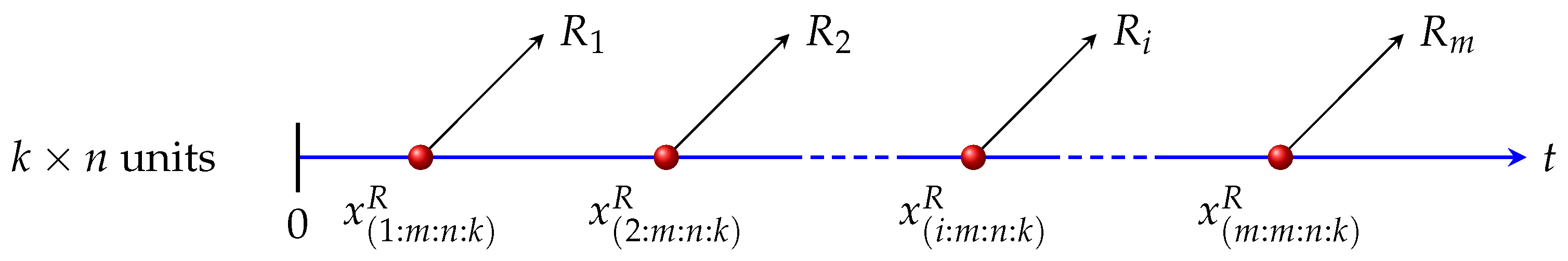
Now, we illustrate the progressive first-failure censoring as follows: Suppose that n groups are being tested simultaneously in a life-testing experiment, every group has k test units and they are totally independent of each other. During the experiment, in time of the occurrence of the first failed component, the group it belongs to and any R 1 groups in the rest of n 1 groups are promptly eliminated from the test. In the same way, in time of the occurrence of the second failed component, the group it belongs to and any R 2 groups in the rest of n 2 R 1 groups are promptly eliminated from the test. This procedure keeps going on until the mth failed component occurs and all the remaining R m groups are immediately eliminated from the test. Here m and R = ( R 1 , R 2 , , R m ) are set in advance and i = 1 m R i + m = n . To further illustrate, Figure 1 shows the process of the generation of progressive first-failure censored sample. In particular, pay attention that this censoring scheme has several special cases, one may refer to [10]. All the conclusions mentioned afterward are available to extend to those kinds of data, which is one of the advantages of progressive first-failure censoring.
The truncated normal distribution is used in many fields, including education, insurance, engineering, biology and medicine, etc. When a threshold is set on a normally distributed dataset, the remaining data naturally have a truncated normal distribution. For instance, when all college admission candidates whose SAT scores are below the screening value are eliminated, people may be interested in the scores of the remaining candidates. However, if the original score population is normally distributed, the problem they concern turns to investigate the truncated normal distribution. Generally speaking, the truncated normal distribution consists of one-sided truncated and two-sided truncated in terms of the number of truncated points. Simultaneously, with respect to the truncation range, the one-sided truncated normal distribution can be subdivided into left-truncated and right-truncated, and they are also known as lower-truncated and upper-truncated.
The truncated normal distribution has recently attracted a lot of research interest. The existence of MLEs for the parameters was discussed in [11] when the two truncated points were known, and the modified MLEs were further explored to improve the efficiency of the estimation. Ref. [12] developed a handy algorithm to compute the expectation and variance of a truncated normally distributed variable and they compared its behavior under both full and censored data. As for the left-truncated normal distribution, Ref. [13] employed three available approaches to investigate the problem of sample size. In addition to the MLEs and Bayes estimators, Ref. [14] also proposed midpoint approximation to derive the estimates of parameters based on progressive type-I interval-censored sample, and meanwhile, the optimal censoring plans were considered. For the purpose of advancing the research on the standardized truncated normal distribution, Ref. [15] developed a standard truncated normal distribution that wherever the truncated points are, it remains the mean value zero and the variance one. Ref. [16] proposed a mixed truncated normal distribution to describe the wind speed distribution and verified its validity.
When it comes to the properties of the truncated normal distribution, it is worth noting that its shape and scale parameters are not equal to its expectation and variance but correspond to the parameters of the parent normal distribution before truncation. After the truncation range is determined, the value of the probability density function outside it becomes zero, while the value within it is adjusted uniformly to make the total integral one. Therefore, expectation and variance are adjusted for the truncation.
Assuming X is a truncated normally distributed random variable and its truncation range is ( a , b ) , the shape and scale parameters are μ and τ , then its expectation and variance correspond to
E ( X ) = μ + ϕ ( a μ τ ) ϕ ( b μ τ ) Φ ( b μ τ ) Φ ( a μ τ ) τ ,
and
V a r ( X ) = 1 + ( a μ τ ) ϕ ( a μ τ ) ( b μ τ ) ϕ ( b μ τ ) Φ ( b μ τ ) Φ ( a μ τ ) ϕ ( a μ τ ) ϕ ( b μ τ ) Φ ( b μ τ ) Φ ( a μ τ ) τ ,
here ϕ ( · ) and Φ ( · ) denote the probability density function (PDF) and cumulative distribution function (CDF) of the standard normal distribution.
Some mechanical and electrical products such as their material strength, wear life, gear bending, and fatigue strength can be considered to have a truncated normal life distribution. As a lifetime distribution, the domain of the random variable should be non-negative and consequently, it is reasonable to assume that x > 0 . Thus, we consider the left-truncated normal distribution with the truncation range ( 0 , ) , denoted as T N ( μ , τ ) , then the corresponding PDF that is f ( x ) and CDF that is F ( x ) of the distribution T N ( μ , τ )  are
f ( x ; μ , τ ) = e 1 2 τ ( x μ ) 2 2 π τ Φ ( μ τ ) , x > 0 , τ > 0 ,
and
F ( x ; μ , τ ) = 1 1 Φ ( x μ τ ) Φ ( μ τ ) , x > 0 , τ > 0 ,
here μ is the shape parameter and τ is the scale parameter. And the survival function is
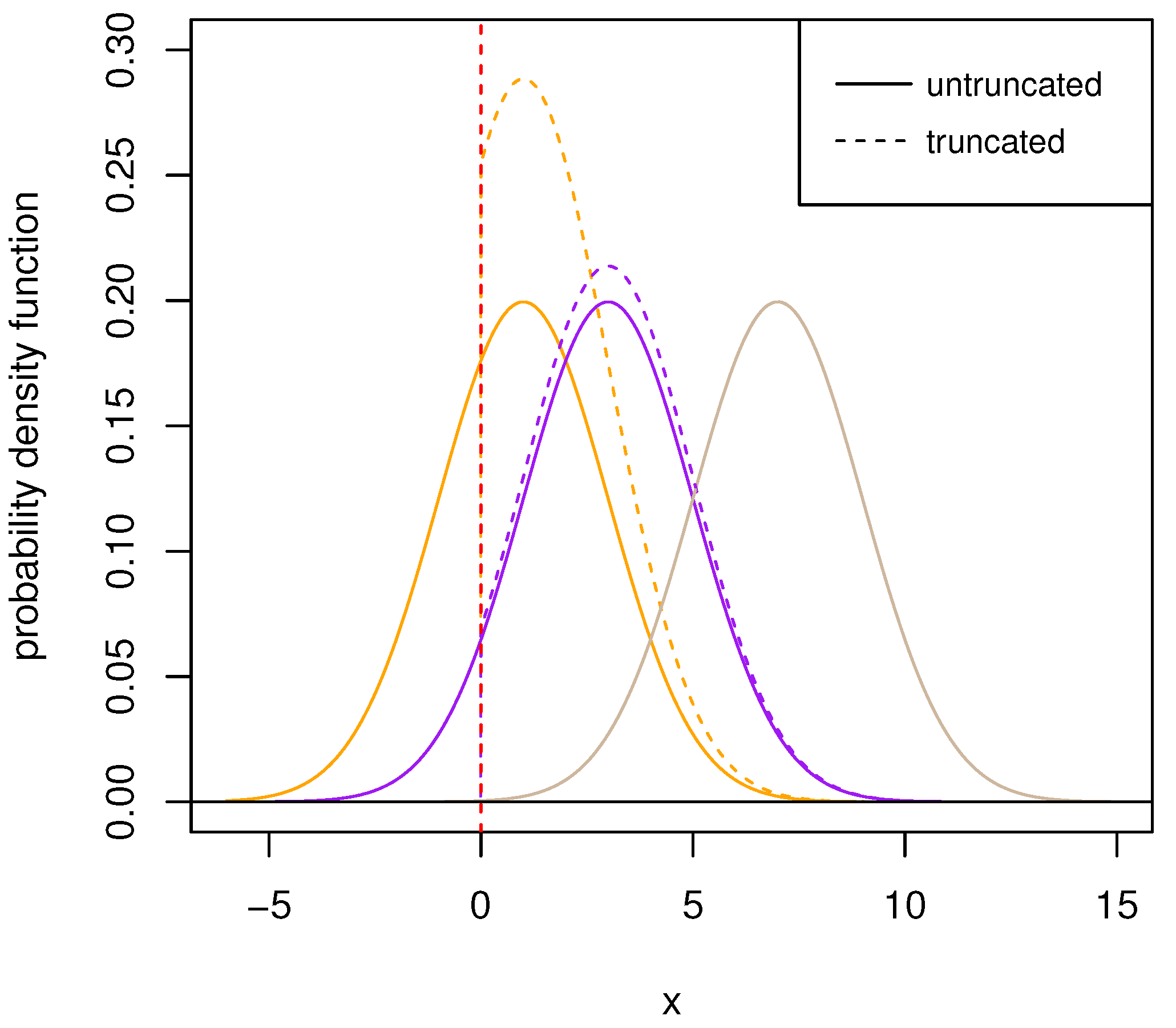
S ( x ; μ , τ ) = 1 Φ ( x μ τ ) Φ ( μ τ ) , x > 0 , τ > 0 .
For comparison, Figure 2 visually shows the distinction of PDFs between three groups of parent normal distributions N ( μ , τ ) and the corresponding truncated normal distribution T N ( μ , τ ) . The parent normal distributions possess the same τ but different μ . Obviously, the parent normal distribution whose shape parameter is closest to the truncated point changes drastically after truncation, while the one with the shape parameter farthest to the truncated point barely changes and even retains the same pattern as normal. In particular, it is worth mentioning that when the truncated point T * satisfies | T * μ | τ 3.5 
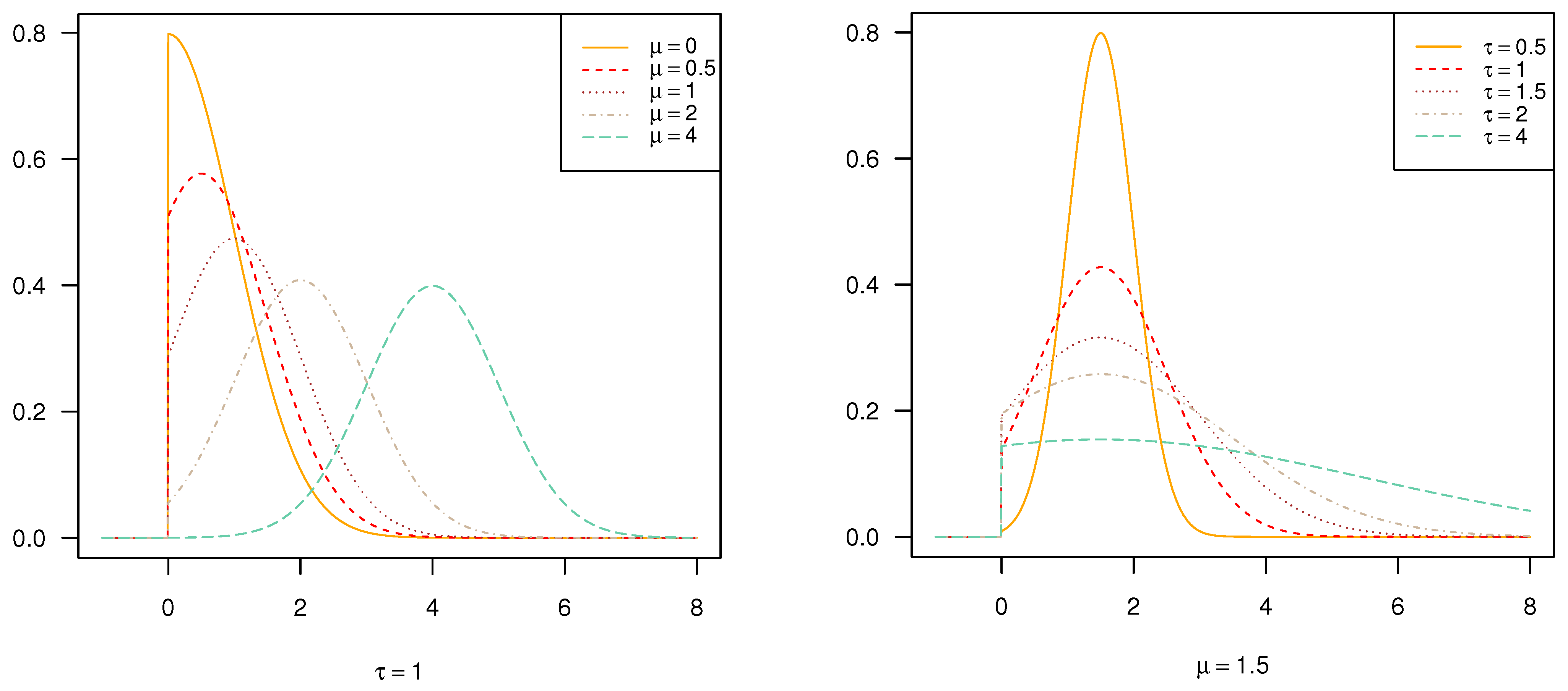
, the truncation basically loses its effect. In Figure 3, we can observe that the position where the peak of the truncated normal distribution occurs is in accordance with the value of μ . As this value gets closer to the truncated point, the peak value of PDF of the distribution T N ( μ , τ ) and the same scale parameter will be larger as a result of the integral of one. However, under the same shape parameters, the image of PDF becomes flat with the increase of scale parameter and it is consistent with the property of normal distribution.
This article begins with the following sections. In the first place, the MLEs for two unknown parameters of the distribution T N ( μ , τ ) are derived in Section 2 and we establish the corresponding asymptotic confidence intervals (ACIs) associated with the approximate asymptotic variance-covariance matrix. In Section 3, the bootstrap resampling method is applied to develop both bootstrap-p and bootstrap-t intervals. In Section 4, we propose the Bayes approaches to estimate two parameters under squared error, Linex, and general entropy loss functions using Lindley approximation. As this approximation method is failed to provide us the credible intervals, the importance sampling procedure is employed to gain both parameter estimates and the highest posterior density (HPD) credible intervals. The behaviors of diverse estimators proposed in the above sections are evaluated and compared by amounts of simulations in Section 5. In Section 6, an authentic dataset is introduced and applied to clarify how to make statistical inferences using the methods presented before and the effectiveness of these approaches. Finally, a summary of the whole article is made in Section 7.

2. Maximum Likelihood Estimation

Suppose that a progressive first-failure type-II censored sample comes from a continuous population with PDF that is f ( · ) and CDF that is F ( · ) . Let’s denote the ith observation as x ( i : m : n : k ) R , thus we have x ( 1 : m : n : k ) R < x ( 2 : m : n : k ) R < < x ( m : m : n : k ) R , here R = ( R 1 , R 2 , , R m ) . For simplicity, let x ̲ = ( x 1 , x 2 , , x m ) replace ( x ( 1 : m : n : k ) R , x ( 2 : m : n : k ) R , , x ( m : m : n : k ) R ) . According to [1,2], the joint PDF is presented as
f X ( 1 : m : n : k ) R , , X ( m : m : n : k ) R ( x 1 , x 2 , x m ) = C k m i = 1 m f ( x i ) ( 1 F ( x i ) ) k ( R i + 1 ) 1 ,
where C = k = 1 m ( n k + 1 l = 0 k 1 R l ) is a normalizing constant, R 0 = 0 , and  0 < x 1 < x 2 < < x m < .
For the case where the sample is from T N ( μ , τ ) , after combining (3), (4) and (6), the likelihood function turns to be
L ( μ , τ | x ̲ ) = C k m i = 1 m e 1 2 ζ i 2 2 π τ Φ ( ζ ) 1 Φ ( ζ i ) Φ ( ζ ) k ( R i + 1 ) 1 ,
where ζ = μ τ , ζ i = x i μ τ .
     Hence, the log-likelihood function is
l ( μ , τ | x ̲ ) = ln C + m ln k i = 1 m 1 2 ζ i 2 m 2 ln ( 2 π τ ) m ln Φ ( ζ ) + i = 1 m [ k ( R i + 1 ) 1 ] [ ln ( 1 Φ ( ζ i ) ) ln Φ ( ζ ) ] .
Take the partial derivatives of (8) concerning μ and τ respectively and set them equal to zero, the corresponding equations are
l μ = N τ ϕ ( ζ ) Φ ( ζ ) + 1 τ i = 1 m ζ i + 1 τ i = 1 m [ k ( R i + 1 ) 1 ] ϕ ( ζ i ) 1 Φ ( ζ i ) = 0 ,
and
l τ = m 2 τ + N ζ 2 τ ϕ ( ζ ) Φ ( ζ ) + 1 2 τ i = 1 m ζ i 2 + 1 2 τ i = 1 m [ k ( R i + 1 ) 1 ] ζ i ϕ ( ζ i ) 1 Φ ( ζ i ) = 0 ,
where N = k × n .
The roots of the non-linear Equations (9) and (10) correspond to the MLEs μ ^ and τ ^ , but the explicit expressions are obviously unobtainable, so some numerical techniques such as Newton-Raphson method are employed to derive the MLEs.

2.1. Asymptotic Confidence Intervals for MLEs

Given that MLEs possess the asymptotic normality, the ACIs of μ and τ can be established by using V a r ( μ ^ ) and V a r ( τ ^ ) . The asymptotic variances of MLEs can be obtained from the inverse Fisher information matrix. Let θ = ( θ 1 , θ 2 ) = ( μ , τ ) . The Fisher information matrix (FIM) I ( θ ) can be written as
I ( θ ) = E 2 l θ 1 , θ 2 θ 1 2 2 l θ 1 , θ 2 θ 1 θ 2 2 l θ 1 , θ 2 θ 2 θ 1 2 l θ 1 , θ 2 θ 2 2 .
Here
2 l ( θ 1 , θ 2 ) θ 1 2 = m τ N τ ( G G 2 ) 1 τ i = 1 m [ k ( R i + 1 ) 1 ] ( G i + G i 2 ) , 2 l ( θ 1 , θ 2 ) θ 1 θ 2 = 2 l ( θ 1 , θ 2 ) θ 2 θ 1 = 1 τ 3 / 2 i = 1 m ζ i + N 2 τ 3 / 2 ( G + ζ G ζ G 2 ) 1 2 τ 3 / 2 i = 1 m [ k ( R i + 1 ) 1 ] ( G i + ζ i G i + ζ i G i 2 ) , 2 l ( θ 1 , θ 2 ) θ 2 2 = 1 τ 2 i = 1 m ζ i 2 + m 2 τ 2 3 N ζ 4 τ 2 G + N ζ 2 4 τ 2 ( G 2 G ) 3 4 τ 2 i = 1 m [ k ( R i + 1 ) 1 ] ζ i G i 1 4 τ 2 i = 1 m [ k ( R i + 1 ) 1 ] ζ i 2 ( G i 2 + G i ) ,
where G = ϕ ( ζ ) Φ ( ζ ) , G = ϕ ( ζ ) Φ ( ζ ) , G i = ϕ ( ζ i ) 1 Φ ( ζ i ) , G i = ϕ ( ζ i ) 1 Φ ( ζ i ) .
     The FIM I ( θ ) is in form of expectation and the acquirement of its exact value depends on the distribution of the order statistics X ( j ) . Ref. [1] provided the PDF of the order statistics X ( j ) of the progressive type-II censored data in general,
f X ( j ) ( x j ) = D i i = 1 j c i j f ( x j ) [ 1 F ( x j ) ] d i 1 ,
where d i = m i + 1 + k = i m R k , D i = i = 1 j d i , c 11 = 1 , c i j = k = 1 , k i j 1 d k d i , 1 i j m .
Since progressive first-failure censoring can be regarded as an extention to the progressive type-II censoring. We can derive the PDF of the order statistics X ( j ) of the truncated normal distribution T N ( μ , τ ) under PFFCS after some transformations of (12), and it is given as
f X ( j ) ( x j ) = D i i = 1 j k c i j e 1 2 τ ( x μ ) 2 2 π τ [ Φ ( μ τ ) ] ( k + 1 ) [ 1 Φ ( x μ τ ) ] k d i 1 ,
Then, the FIM I ( θ ) can be calculated directly based on (13). In practice, the expectation in (11) can be removed naturally and the observed FIM I ( θ ^ ) is used to approximate the asymptotic variance-covariance matrix for the purpose of simplifying the complicated calculation, see [2,17]. The observed FIM I ( θ ^ ) corresponds to
I ( θ ^ ) = 2 l θ 1 , θ 2 θ 1 2 2 l θ 1 , θ 2 θ 1 θ 2 2 l θ 1 , θ 2 θ 2 θ 1 2 l θ 1 , θ 2 θ 2 2 θ = θ ^ ,
here, θ ^ denotes the MLE of θ , namely θ ^ = ( θ ^ 1 , θ ^ 2 ) = ( μ ^ , τ ^ ) .
Then the approximate asymptotic variance-covariance matrix is
I 1 ( θ ^ ) = V a r ^ ( μ ^ ) C o v ^ ( μ ^ , τ ^ ) C o v ^ ( τ ^ , μ ^ ) V a r ^ ( τ ^ ) .
Therefore, the  100 ( 1 ξ ) % ACI for θ j is given by
θ j ^ z ξ / 2 I 1 ( θ ^ ) j j , θ j ^ + z ξ / 2 I 1 ( θ ^ ) j j , j = 1 , 2 ,
where z ξ / 2 is the ξ / 2 upper quantile of the standard normal distribution.

2.2. Asymptotic Confidence Intervals for Log-Transformed MLEs

The method just proposed has an obvious defect that its lower bound of ACI is prone to appear negative value when the truth value of the parameter is small. Since the parameter τ discussed in this paper is strictly non-negative, the negative part of the confidence interval is unreasonable at that time. To avoid this issue, we can use delta method and logarithmic transformation proposed in [18]. Similarly, this method is available to μ when μ > 0 . The asymptotic distribution of ln θ j ^ is
ln θ j ^ ln θ j D N ( 0 , v a r ( ln θ j ^ ) ) ,
where D denotes convergence in distribution and v a r ( ln θ j ^ ) = v a r ( θ j ^ ) θ j ^ 2 v a r ^ ( θ j ^ ) θ j ^ 2 = I 1 ( θ ^ ) j j θ j ^ 2 .
    Therefore, the asymptotic confidence intervals based on log-transformed MLEs are
θ j ^ exp z ξ / 2 θ j ^ v a r ^ ( θ j ^ ) , θ j ^ exp z ξ / 2 θ j ^ v a r ^ ( θ j ^ ) , j = 1 , 2 .
The proposal of these two ACIs is on the premise that MLEs are asymptotically normally distributed. Hence, if the number of the sample is not large enough, the accuracy of these two confidence intervals may be declined. In the next section, we provide a resampling technique to solve the problem of building confidence intervals for parameters under a small sample size.

3. Bootstrap Confidence Intervals

Bootstrap methods can make great sense in the case with little effective sample size m, so here we propose two widely used bootstrap methods to establish the intervals, see [19]. One is the percentile bootstrap method, also regarded as bootstrap-p (boot-p). The other is known as the bootstrap-t (boot-t) method. The specific steps of the two methods are as follows.

3.1. Percentile Bootstrap Confidence Intervals

Step 1 For a given PFF censored sample x ̲ from T N ( μ , τ ) with n , m , k and R = ( R 1 , R 2 , , R m ) , figure the MLEs of parameters μ and τ under the primitive sample x ̲ , denoted as μ ^ and τ ^ .
Step 2 In accordance with the identical censoring pattern ( n , m , k , R ) as x ̲ , generate a PFF censored bootstrap sample x ̲ * from T N ( μ ^ , τ ^ ) . Similarly to step 1, compute the bootstrap MLEs μ ^ * and τ ^ * based on x ̲ * .
Step 3 Do step 2 repeatedly for K times to collect a series of bootstrap MLEs μ ^ j * and τ ^ j * ( j = 1 , 2 , , K ) .
Step 4 Arrange μ ^ j * and τ ^ j * in an ascending order respectively then obtain ( μ ^ ( 1 ) * , μ ^ ( 2 ) * , , μ ^ ( K ) * ) and ( τ ^ ( 1 ) * , τ ^ ( 2 ) * , , τ ^ ( K ) * ) .
Step 5 The approximate 100 ( 1 ξ ) % boot-p CIs for μ and τ are presented by ( μ ^ ( α 1 ) * , μ ^ ( α 2 ) * ) and ( τ ^ ( α 1 ) * , τ ^ ( α 2 ) * ) , where α 1 and α 2 are respectively the integer parts of K × ( ξ / 2 ) and K × ( 1 ξ / 2 ) .

3.2. Bootstrap-t Confidence Intervals

Step 1 For a given PFF censored sample x ̲ from T N ( μ , τ ) with n , m , k and R = ( R 1 , R 2 , , R m ) , figure the MLEs μ ^ and τ ^ and their variances V a r ^ ( μ ^ ) and V a r ^ ( τ ^ ) under the primitive sample x ̲ .
Step 2 In accordance with the identical censoring pattern ( n , m , k , R ) as x ̲ , generate a PFF censored bootstrap sample x ̲ * from T N ( μ ^ , τ ^ ) . Similarly to step 1, compute the bootstrap MLEs μ ^ * and τ ^ * based on x ̲ * .
Step 3 Compute the variances of μ ^ * and τ ^ * , say V a r ^ ( μ ^ * ) and V a r ^ ( τ ^ * ) , then compute the statistics U * = μ ^ * μ ^ V a r ^ ( μ ^ * ) for μ ^ * and V * = τ ^ * τ ^ V a r ^ ( τ ^ * ) for τ ^ * .
Step 4 Do steps 2-3 repeatedly for K times to collect a series of bootstrap statistics U j * and V j * ( j = 1 , 2 , , K ) .
Step 5 Arrange U j * and V j * in an ascending order respectively then obtain ( U ( 1 ) * , U ( 2 ) * , , U ( K ) * ) and ( V ( 1 ) * , V ( 2 ) * , , V ( K ) * ) .
Step 6 The approximate 100 ( 1 ξ ) % boot-t CIs for μ and τ are presented by
μ ^ U [ α 2 ] * V a r ^ ( μ ^ ) , μ ^ U [ α 1 ] * V a r ^ ( μ ^ ) , τ ^ V [ α 2 ] * V a r ^ ( τ ^ ) , τ ^ V [ α 1 ] * V a r ^ ( τ ^ ) ,
where α 1 and α 2 are respectively the integer parts of K × ( ξ / 2 ) and K × ( 1 ξ / 2 ) .

4. Bayesian Estimation

The selection of prior distribution is a primary problem of Bayesian estimation for the fact that the prior distribution could have a significant impact on the posterior distribution in small sample cases. So, a proper prior distribution is worth discussing at the beginning.
In general cases, the conjugate prior distribution is a preferred choice in Bayesian estimation because of its algebraic convenience. However, such prior does not exist when both parameters μ and τ are unknown. For the sake of simplicity, we need to find a prior distribution with the same form as (7). Furthermore, according to the form of the denominator part of the exponential term in the likelihood function (7), τ should appear as a parameter of the prior distribution of μ . Therefore, assuming that they are not independent is feasible and we can presume that τ follows an Inverse Gamma prior I G ( α , β ) and μ follows a truncated normal prior associated with τ , namely μ T N ( a , τ b ) , where all hyper-parameters are bound to be positive. The PDFs of their prior distributions can be written as
π 1 ( τ ) = β α Γ ( α ) τ α 1 e β τ ,
π 2 ( μ | τ ) = e b 2 τ ( μ a ) 2 2 π τ b Φ ( a b τ ) .
The corresponding joint prior distribution is
π ( μ , τ ) = π 1 ( τ ) π 2 ( μ | τ ) 1 Φ a b τ 1 τ α + 3 2 e 1 2 τ [ b ( μ a ) 2 + 2 β ] .
Given x ̲ , the joint posterior distribution π ( μ , τ | x ̲ ) can be obtained by
π ( μ , τ | x ̲ ) = L ( x ̲ | μ , τ ) π ( μ , τ ) 0 0 L ( x ̲ | μ , τ ) π ( μ , τ ) d μ d τ .

4.1. Symmetric and Asymmetric Loss Functions

The loss function is used to evaluate the degree to which the predicted value or the estimated value of the parameter is different from the real value. In practice, the squared error loss function has been used extensively in the literature and it is preferred in the case where the loss caused by overestimation and underestimation is of equal importance. But sometimes, it is not appropriate to use a symmetric loss function when an overestimate plays a crucial role compared with an underestimate, or vice versa. Thus, in this subsection, we discuss the Bayesian estimations theoretically under one symmetric loss function, namely squared error loss function (SE), and two non-symmetric loss functions, namely Linex loss function (LX) and general entropy loss function (GE).

4.1.1. Squared Error Loss Function

This loss function is defined as
L S E ( ϑ , ϑ ^ ) = ( ϑ ^ ϑ ) 2 ,
here, ϑ ^ denotes any estimate of ϑ .
The Bayesian estimator of ϑ under SE is
ϑ ^ S E = E ϑ ( ϑ | x ̲ ) .
Given a function g ( μ , τ ) , the expression of its Bayesian posterior expectation is
E [ g ( μ , τ ) | x ̲ ] = 0 0 g ( μ , τ ) L ( x ̲ | μ , τ ) π ( μ , τ ) d μ d τ 0 0 L ( x ̲ | μ , τ ) π ( μ , τ ) d μ d τ .
Thus, the Bayesian estimate g ^ ( μ , τ ) under SE can be given theoretically as
g ^ ( μ , τ ) S E = 0 0 g ( μ , τ ) L ( x ̲ | μ , τ ) π ( μ , τ ) d μ d τ 0 0 L ( x ̲ | μ , τ ) π ( μ , τ ) d μ d τ .

4.1.2. Linex Loss Function

The Linex loss function is suggested in the case that underestimation is more costly compared with overestimation, and this loss function is defined as
L ( Δ ) = b [ e a Δ a Δ 1 ] , a 0 , b > 0 .
In fact, it is recognized as a family L ( Δ ) where Δ could be either the usual estimation error ϑ ^ ϑ or a relative error ( ϑ ^ ϑ ) / ϑ , namely ϑ ^ ϑ 1 . In this paper, we take advantage that Δ = ϑ ^ ϑ and let b = 1 , then LX becomes
L L X ( ϑ , ϑ ^ ) = e s ( ϑ ^ ϑ ) s ( ϑ ^ ϑ ) 1 , s 0 .
The sign of the s indicates the orientation of asymmetry, while its size represents the degree of asymmetry. Under the same difference ϑ ^ ϑ , the larger the magnitude of s is, the larger the cost is. Given small values of | s | , LX is almost symmetric and very close to SE. One may refer to [20] for details.
The Bayesian estimator of ϑ under LX is
ϑ ^ L X = 1 s ln E ϑ ( e s ϑ | x ̲ ) .
Thus, the Bayesian estimate g ^ ( μ , τ ) under LX can be given theoretically as
g ^ ( μ , τ ) L X = 1 s ln 0 0 e s g ( μ , τ ) L ( x ̲ | μ , τ ) π ( μ , τ ) d μ d τ 0 0 L ( x ̲ | μ , τ ) π ( μ , τ ) d μ d τ .

4.1.3. General Entropy Loss Function

This loss function is defined as
L G E ( ϑ , ϑ ^ ) = ϑ ^ ϑ h h ln ϑ ^ ϑ 1 .
The Bayesian estimator of ϑ under GE is
ϑ ^ G E = E ϑ ( ϑ h | x ̲ ) 1 h .
When h > 0 , the positive error value ϑ ^ ϑ is more costly compared with the negative error value, and vice versa. In particular, when h = 1 , the Bayesian estimate under SE is the same as that under GE.
The Bayesian estimate g ^ ( μ , τ ) under GE can be given theoretically as
g ^ ( μ , τ ) G E = 0 0 g ( μ , τ ) h L ( x ̲ | μ , τ ) π ( μ , τ ) d μ d τ 0 0 L ( x ̲ | μ , τ ) π ( μ , τ ) d μ d τ 1 h .
It is noticeable that the Bayesian estimates are expressed in terms of the ratio of two integrals and the specific forms cannot be presented theoretically. So, we implement the Lindley approximation method to determine such estimates.

4.2. Lindley Approximation Method

In this subsection, we take advantage of Lindley approximation to acquire the Bayesian parameter estimates. Consider the posterior expectation of φ ( μ , τ ) expressed in terms of the ratio of two integrals
E ( φ ( μ , τ ) | x ) = φ ( μ , τ ) e l ( μ , τ ) + ρ ( μ , τ ) d μ d τ e l ( μ , τ ) + ρ ( μ , τ ) d μ d τ ,
here, l denotes the log-likelihood function, ρ denotes the logarithmic form of the joint prior distribution.
According to [21], expression (34) can be approximated as
E ( φ ( μ , τ ) | x ) = φ ( μ ^ , τ ^ ) + 1 2 ( A + l 30 B 12 + l 21 C 12 + l 12 C 21 + l 03 B 21 ) + ρ 1 A 12 + ρ 2 A 21 ,
with
A = i = 1 2 j = 1 2 φ i j σ i j , l i j = i + j l θ 1 i θ 2 j , i , j = 0 , 1 , 2 , 3  and  i + j = 3 ,  
ρ i = ρ θ i , φ i = φ θ i , φ i j = 2 φ θ i θ j , σ i j = [ l i j ] 1 , A i j = φ i σ i i + φ j σ j i ,
B i j = ( φ i σ i i + φ j σ i j ) σ i i , C i j = 3 φ i σ i i σ i j + φ j ( σ i i σ j j + 2 σ i j 2 ) .
     Here θ = ( θ 1 , θ 2 ) = ( μ , τ ) , σ i j denotes the ( i , j ) -th element of the inverse FIM. All terms in (35) are computed at MLEs μ ^ and τ ^ . Then the approximate solution expressions of Bayesian parameter estimates under loss functions SE, LX, and GE are as follows.

4.2.1. Squared Error Loss Function

For parameter μ , we take φ ( μ , τ ) = μ , hence
φ ( μ , τ ) = μ , φ 1 = 1 , φ 11 = φ 12 = φ 2 = φ 21 = φ 22 = 0 .
The Bayesian estimate of μ under SE is derived by combining (24), (35) and (36)
μ ^ S E = μ ^ + 1 2 σ 11 2 l 30 + 3 σ 11 σ 12 l 21 + σ 11 σ 22 l 12 + 2 σ 21 2 l 12 + σ 21 σ 22 l 03 + ρ 1 σ 11 + ρ 2 σ 12 .
Similarly, for parameter τ , we take φ ( μ , τ ) = τ , hence
φ ( μ , τ ) = τ , φ 2 = 1 , φ 21 = φ 22 = φ 1 = φ 11 = φ 12 = 0 .
The Bayesian estimate of μ under SE is derived by combining (24), (35) and (38)
τ ^ S E = τ ^ + 1 2 σ 11 σ 12 l 30 + σ 11 σ 22 l 21 + 2 σ 12 2 l 12 + 3 σ 21 σ 22 l 12 + σ 22 2 l 03 + ρ 1 σ 21 + ρ 2 σ 22 .

4.2.2. Linex Loss Function

For parameter μ , it is clear that
φ ( μ , τ ) = e s μ , φ 1 = s e s μ , φ 11 = s 2 e s μ , φ 12 = φ 2 = φ 21 = φ 22 = 0 .
The Bayesian estimate of μ under LX is derived by combining (29), (35) and (40)
μ ^ L X = 1 s log { e s μ ^ + 0.5 φ 11 σ 11 + 0.5 φ 1 [ σ 11 2 l 30 + 3 σ 11 σ 12 l 21 + σ 11 σ 22 l 12 + 2 σ 21 2 l 12 + σ 21 σ 22 l 03 ] + φ 1 ( ρ 1 σ 11 + ρ 2 σ 12 ) } .
For parameter τ , it is clear that
φ ( μ , τ ) = e s τ , φ 2 = s e s τ , φ 22 = s 2 e s τ , φ 1 = φ 11 = φ 12 = φ 21 = 0 .
The Bayesian estimate of τ under LX is derived by combining (29), (35) and (42)
τ ^ L X = 1 s log { e s τ ^ + 0.5 φ 22 σ 22 + 0.5 φ 2 [ σ 11 σ 12 l 30 + σ 11 σ 22 l 21 + 2 σ 12 2 l 21 + 3 σ 21 σ 22 l 12 + σ 22 2 l 03 ] + φ 2 ( ρ 1 σ 21 + ρ 2 σ 22 ) } .

4.2.3. General Entropy Loss Function

For parameter μ , the corresponding items become
φ ( μ , τ ) = μ h , φ 1 = h μ h 1 , φ 11 = h ( h + 1 ) μ h 2 , φ 12 = φ 2 = φ 21 = φ 22 = 0 .
The Bayesian estimate of μ under GE is derived by combining (32), (35) and (44)
μ ^ G E = { μ ^ h + 0.5 φ 11 σ 11 + 0.5 φ 1 [ σ 11 2 l 30 + 3 σ 11 σ 12 l 21 + σ 11 σ 22 l 12 + 2 σ 21 2 l 12 + σ 21 σ 22 l 03 ] + φ 1 ( ρ 1 σ 11 + ρ 2 σ 12 ) } 1 h .
For parameter τ , the corresponding items become
φ ( μ , τ ) = τ h , φ 2 = h τ h 1 , φ 22 = h ( h + 1 ) τ h 2 , φ 1 = φ 11 = φ 12 = φ 21 = 0 .
The Bayesian estimate of τ under GE is derived by combining (32), (35), and (46)
τ ^ G E = { τ ^ h + 0.5 φ 22 σ 22 + 0.5 φ 2 [ σ 11 σ 12 l 30 + σ 11 σ 22 l 21 + 2 σ 12 2 l 21 + 3 σ 21 σ 22 l 12 + σ 22 2 l 03 ] + φ 2 ( ρ 1 σ 21 + ρ 2 σ 22 ) } 1 h .
When it comes to estimating the ratio of two integrals in the form given in (34), the Lindley approximation method is very effective. Nevertheless, one of its drawbacks is that this method only provides point estimates but not the credible intervals. Therefore, in the upcoming subsection, we propose the importance sampling procedure to gain both estimations of points and intervals.

4.3. Importance Sampling Procedure

Here, we propose a useful approach called importance sampling procedure to acquire the Bayesian parameter estimates. Meanwhile, the HPD credible intervals for both parameters are constructed in this procedure.
From (22), the joint posterior distribution can be rewritten as
π ( μ , τ | x ̲ ) Φ ( μ τ ) N Φ a b τ 1 τ α + m + 3 2 e 1 2 τ [ b ( μ a ) 2 + 2 β + i = 1 m ( x i μ ) 2 ] × i = 1 m 1 Φ x i μ τ k ( R i + 1 ) 1 = I G τ α + m 2 , 1 2 c 2 b + m + a 2 b + 2 β + i = 1 m x i 2 T N μ | τ c b + m , τ b + m ω ( μ , τ ) = I G τ ( α ˜ , β ˜ ) T N μ | τ ( a ˜ , τ b ˜ ) ω ( μ , τ ) ,
where
c = a b + i = 1 m x i , ω ( μ , τ ) = Φ ( μ τ ) N Φ ( a b τ ) Φ a b + i = 1 m x i τ ( b + m ) i = 1 m 1 Φ ( x i μ τ ) k ( R i + 1 ) 1 .
According to the Lemma 1, the parameters of the inverse gamma distribution and the truncated normal distribution in (48) are positive. Thus, it makes sense to sample τ from I G τ ( α ˜ , β ˜ ) the and sample μ from T N μ | τ ( a ˜ , τ b ˜ ) .
Lemma 1.
If a , b , β > 0 and m 1 , then ( a b + i = 1 m x i ) 2 b + m + a 2 b + 2 β + i = 1 m x i 2 > 0 for all x = { ( x 1 , x 2 , , x m ) : x i R ,  for i = 1 , 2 , m } .
Proof. 
According to the sum of squares inequality, we can get ( i = 1 m x i ) 2 m i = 1 m x i 2 .
( a b + i = 1 m x i ) 2 b + m + a 2 b + 2 β + i = 1 m x i 2 > 0 2 a b i = 1 m x i + ( i = 1 m x i ) 2 2 b β + a 2 b m + 2 β m + ( m + b ) i = 1 m x i 2 .
Because
m + b m ( i = 1 m x i ) 2 < ( m + b ) i = 1 m x i 2 ,
then we must prove the non-negativeness of the following quadratic function when we regard i = 1 m x i as the independent variable of it.
b m ( i = 1 m x i ) 2 2 a b i = 1 m x i + 2 b β + a 2 b m + 2 β m > 0 .
Notably, the quadratic function above minimizes at ( i = 1 m x i ) 2 = a m , and the corresponding result is 2 β ( b + m ) , which is strictly non-negative. Thus, the lemma is proved.
   □
Then, the following steps are used to derive the Bayesian estimate of any function Ω ( μ , τ ) of the parameters μ and τ .
(1)
Generate τ from I G τ α + m 2 , 1 2 ( a b + i = 1 m x i ) 2 b + m + a 2 b + 2 β + i = 1 m x i 2 .
(2)
Generate μ from T N μ | τ a b + i = 1 m x i b + m , τ b + m with the τ generated in (1).
(3)
Repeat (1) and (2) M times and get the sample ( μ 1 , τ 1 ) , ( μ 2 , τ 2 ) , , ( μ M , τ M ) .
(4)
Then the Bayesian estimate of Ω ( μ , τ ) is computed by
Ω ^ ( μ , τ ) = i = 1 M Ω ( μ i , τ i ) ω ( μ i , τ i ) i = 1 M ω ( μ i , τ i ) .
Considering the unknown parameters μ and τ , their Bayesian estimates could be derived by
μ ^ = i = 1 M μ i ω ( μ i , τ i ) i = 1 M ω ( μ i , τ i ) , τ ^ = i = 1 M τ i ω ( μ i , τ i ) i = 1 M ω ( μ i , τ i ) .
Next the HPD credible interval for parameter μ is illustrated, while the corresponding HPD credible interval for τ can be computed by the same method. Let
v i = ω ( μ i , τ i ) i = 1 M ω ( μ i , τ i ) , i = 1 , 2 , , M .
Then we sort { ( μ 1 , v 1 ) , ( μ 2 , v 2 ) , , ( μ M , v M ) } by the first component μ in ascending order and we can get { ( μ ( 1 ) , v ( 1 ) ) , ( μ ( 2 ) , v ( 2 ) ) , , ( μ ( M ) , v ( M ) ) } . Here v ( i ) is associated with μ ( i ) , which means that v ( i ) is not ordered. The construction of HPD credible interval is based on an estimate μ ^ p and μ ^ p = μ ( C p ) , where C p is an integer that satisfies
i = 1 C p v ( i ) p i = 1 C p + 1 v ( i ) .
Now, a  100 ( 1 ξ ) % credible interval for the unknown parameter μ can be acquired as ( μ ^ δ , μ ^ δ + 1 ξ ) , δ = v ( 1 ) , v ( 1 ) + v ( 2 ) , , i = 1 N 1 ξ v ( i ) . Therefore, the corresponding HPD credible interval for μ is given by
( μ ^ δ * , μ ^ δ * + 1 ξ ) ,
where μ ^ δ * + 1 ξ μ ^ δ * μ ^ δ + 1 ξ μ ^ δ  for all δ .

5. Simulation Study

For evaluating the effectiveness of the proposed methods, plenty of simulations are carried out in this part. The maximum likelihood and Bayes estimators proposed above are assessed based on the mean absolute bias (MAB) and mean squared error (MSE), whereas interval estimations are considered according to the mean length (ML) and coverage rate (CR). Looking back to the progressive first-failure censoring presented in the first part, it can be found that when an experimental group is regarded as one unit, the life of this experimental unit turns into the life distribution of the minimum value of the group. In this way, it is intelligible to generate PFF censored sample through a simple modification of the algorithm introduced in [22] and Algorithm 1 given subsequently provides the specific generation method.
Algorithm 1 Generating progressive first-failure censored sample from T N ( μ , τ )
1. 
Set the initial values of both group size k and censoring scheme R = ( R 1 , R 2 , , R m ) .
2. 
Generate independent random variables Z 1 , Z 2 , , Z m that obey the uniform distribution U ( 0 , 1 ) .
3. 
Let Y i = Z i 1 i + R m + + R m i + 1 for all i { 1 , 2 , , m } .
4. 
Let U i = 1 Y m Y m 1 Y m i + 1 for all i { 1 , 2 , , m } .
5. 
For given μ and τ , let H ( x ) = 1 ( 1 F ( x ) ) k , here F ( x ) represents the CDF of T N ( μ , τ ) .
6. 
Finally, we set X i = H 1 ( U i ) for all i { 1 , 2 , , m } , here H 1 ( · ) represents the inverse function of H ( · ) . Hence, X = ( X 1 , X 2 , , X m ) is the PFF censored sample from T N ( μ , τ ) .
Here, we take the true values of parameters as μ = 3 and τ = 1 . For comparison purposes, we consider k = 1 , 2 , n = 30 , 40 and m = 40 % n , 70 % n , 100 % n . Meanwhile, different censoring schemes (CS) designed for the later simulations are presented in Table 1. As a matter of convenience, we abbreviate the censoring scheme to make it clear, for instance, ( 0 * 5 ) is the abbreviation of the censoring scheme ( 0 , 0 , 0 , 0 , 0 ) . In each case, we repeat the simulation at least 2000 times. Thus, the associated MABs and MSEs with the point estimation and the associated MLs and CRs with the interval estimation can be obtained.
First, it should be noted that all our simulations are performed in R software. For maximum likelihood estimation, we use optim command with method L-BFGS-B to derive the MLEs of parameters, and then we tabulate the corresponding results in Table 2. For Bayesian estimation, we naturally consider the true value as the mean of the prior distribution. But such hyper-parameters are intractable because of the complexity of prior distribution. Therefore, we use genetic algorithm and mcga package in R software to search for the optimal hyper-parameters and the result turns out to be a = 4 , b = 2 , α = 5.5 , β = 2.5 . Then two Bayes approaches with informative prior are implemented to derive the estimates under loss functions SE, LX and GE. We set the parameter s of LX to 0.5 and 1, while the parameter h of GE is 0.5 and 0.5 . These simulation results are listed in Table 3, Table 4, Table 5 and Table 6.
At the same time, the proposed intervals are established at 95% confidence/credible level and Table 7 and Table 8 summarize the results. Here, ACI denotes asymptotic confidence interval based on MLEs, Log-ACI denotes the asymptotic confidence interval based on log-transformed MLEs. In the following simulations, the bootstrap confidence intervals are obtained after K = 1000 resamples while HPD credible intervals are obtained after M = 1000 samples.
From Table 2, we can observe some properties about maximum likelihood estimates:
(1)
The maximum likelihood estimate of μ performs much better than that of the maximum likelihood estimate of τ with respect to MABs and MSEs.
(2)
When the effective sample size m or the total number of groups n or the value of m / n increases, MABs and MSEs decrease significantly for all estimators, which is exactly as we expected. With the increasing group size k, MABs and MSEs generally decrease for the shape parameter μ , while the corresponding indicators generally increase for the scale parameter τ .
(3)
Different censoring schemes show a certain pattern as for MABs and MSEs. For μ , both are generally smaller under the middle censoring schemes, on the contrary, both are generally smaller under the left censoring schemes for τ .
From Table 3, Table 4, Table 5 and Table 6, we can observe that:
(1)
Under three loss functions, the Bayesian estimates with proper prior are more accurate than MLEs as for MABs and MSEs in all cases. Both Bayesian methods are better than MLEs undoubtedly and it is clear that the Lindley approximation outperforms the importance sampling.
(2)
Few censoring schemes such as r 2 and r 7 do not compete well for the Bayesian estimation of τ . The commonality of these two schemes is that they own the small effective sample size m and both are middle censorings.
(3)
The Bayesian estimates of τ under SE is superior compared with GE, while the Bayesian estimates of μ under SE is similar to GE. For GE, choosing h = 0.5 is better than h = 0.5 . For LX, both s = 0.5 and s = 1 are satisfactory and they compete quite well. Overall, the Bayes estimates under Linex loss function using Lindley approximation are highly recommended as it possesses the minimum of MABs and MSEs.
From Table 7 and Table 8, we can conclude that:
(1)
In general, the ML of HPD credible interval is the most satisfying compared with the other intervals, while the boot-t confidence interval possesses the widest ML. With the increase of m / n , the ML shows a tendency to narrow, and this pattern holds for both parameters.
(2)
Boot-p confidence interval is unstable as its CR decreases significantly when the group size k increases, whereas boot-t interval is basically not affected by k and possesses the robustness to some extent considering μ .
(3)
ACI competes well with Log-ACI for μ and they are similar in terms of ML and CR. However, the CR of Log-ACI is much improved and more precise than ACI for τ . Therefore, Log-ACI seems to be a better choice.

6. Authentic Data Analysis

Now, we introduce an authentic dataset and we analyze it by using the methods developed above. This dataset was obtained from [23], which was analyzed in [5,24] respectively. This dataset, presented in Table 9, describes the tensile strength of 100 tested 50mm carbon fibers and it is measured in giga-Pascals (GPa).
First, we test whether the distribution T N ( μ , τ ) fits this real dataset well. In particular, Ref. [24] compared the fitting results with many famous reliability distributions, such as Rayleigh distribution, and Log-Logistic distribution, etc. They concluded that Log-Logistic distribution has the best fitting effect. Therefore, we compare the fitting effect of truncated normal distribution and Log-Logistic distribution with the PDF that is g ( x ) = β α ( x α ) β 1 / ( 1 + ( x α ) β ) 2 , x > 0 .
Various criteria are applied for testing the goodness of fit of the model, such as the negative log-likelihood function ln L , Akaike Information Criterion (AIC), Bayesian Information Criterion (BIC), and Kolmogorov–Smirnov (K-S) statistics with its p-value. The corresponding definitions of the above criteria are given as
A I C = 2 × ( d ln L d ( x 1 , , x n | θ ) ) , B I C = d × ln n 2 × ln L d ( x 1 , , x n | θ ) ,
here, θ is a parameter vector, d is the number of parameters in the fitted model, ln L d is evaluated at the MLEs, and n is the number of observed values.
Table 10 shows the MLEs of the parameters for each distribution, along with ln L , AIC, BIC, K-S, and p-value corresponding to two distributions. Conspicuously, since the truncated normal distribution has the lower statistics and higher p-value, it does fit the complete sample well. Now, we can use this dataset for analysis.
Therefore, we randomly divide the given data into 50 groups, and each group has two independent units. Thus, the first-failure censored data are obtained, as shown in Table 11. In order to gain the PFF censored samples, we set m = 25 and give three different kinds of censoring schemes, namely c 1 = ( 25 , 0 * 24 ) , c 2 = ( 1 * 25 ) , c 3 = ( 0 * 24 , 25 ) . Table 12 presents the PFF censored samples under left censoring, middle censoring and right censoring.
In Table 13 and Table 14, the point estimates of parameters μ and τ are shown, respectively. No informative prior is available for Bayesian estimation, so we apply non-informative prior, and the four hyper-parameters are all around zero tightly and three loss functions discussed before are taken into account. As for the two asymmetric loss functions, we continue to use the parameters in the previous simulations, namely s = 0.5 and s = 1 , h = 0.5 and h = 0.5 . It can be seen from the table that there are some differences between the estimated values obtained by different censoring schemes and different methods. The parameter estimates based on censoring scheme c 1 are closest to the MLEs under the full sample, while the estimates using the importance sampling are pervasively inclined to be smaller compared with those gained by Lindley approximation. At the same time, we construct 95 % ACIs, Log-ACIs, bootstrap, and HPD intervals, while Table 15 and Table 16 display the corresponding results.
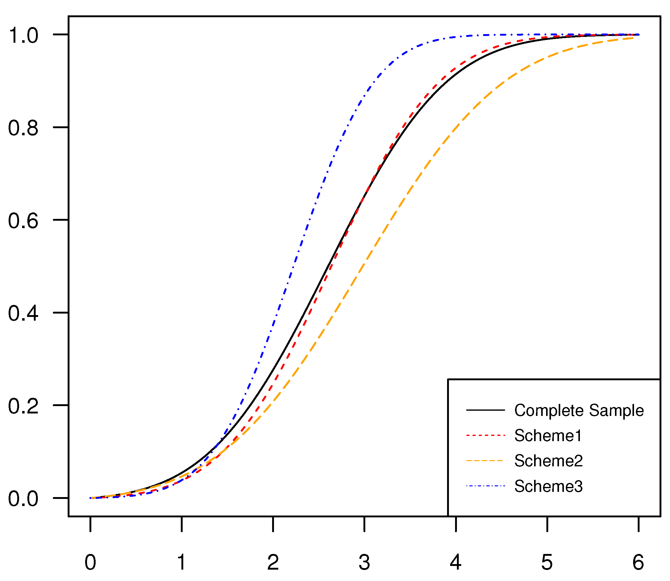
In Figure 4, we have drawn four different estimated distribution function images, and their corresponding parameters are MLEs under complete samples and censored samples with schemes c 1 , c 2 and c 3 . It is of considerable interest to see that the estimated curve based on the censoring scheme c 1 = ( 25 , 0 * 24 ) is the closest to the estimated curve based on full data, which indicates that the left censored data is the superior one. In the middle part of the graphics, we can tell that the value of the estimated curve is underestimated based on the censoring scheme c 2 = ( 1 * 25 ) , and on the contrary, the value based on the censoring scheme c 3 = ( 0 * 24 , 25 ) is overestimated.

7. Conclusions

Throughout the full article, we consider the classical and Bayesian inference for a progressive first-failure censored left-truncated normal distribution. MLEs are derived using an optimization technique and the Bayesian estimation is taken into account under loss functions SE, LX, and GE. At the same time, confidence and credible intervals for the parameters are constructed and compared with each other. In the simulation section, MAB and MSE are taken into account for the point estimation while the ML and CR are considered for the interval estimation.
When it comes to the point estimation, the performance of MLEs is satisfactory, whereas the Bayesian estimation with proper informative prior is superior to MLEs in all cases. According to the simulation study presented in this paper, the Bayesian estimates with proper prior under loss function LX are the best among all estimates, and Lindley approximation method is highly recommended. Moreover, in terms of interval estimation, ACIs based on log-transformed MLEs have more accurate coverage rate than ACIs based on MLEs. HPD credible intervals consistently have the shortest interval length compared with other confidence intervals.
The truncated normal distribution is versatile as it possesses the flexibility of truncation and the superior properties of normal distribution. The research object in this article is a progressive first-failure censored left-truncated normal distribution with a known truncated point. In some cases, we may be interested in the position of the truncated point so it is inevitable to estimate the unknown truncated point. Furthermore, the research field of this censoring plan adding with binomial removals and competing risks can be explored. In brief, it is still of great potential to conduct further research of truncated normal distribution.

Author Contributions

Investigation, Y.C.; Supervision, W.G. Both authors have read and agreed to the published version of the manuscript.

Funding

This research was supported by Project 202110004003 which was supported by National Training Program of Innovation and Entrepreneurship for Undergraduates.

Conflicts of Interest

The authors declare no conflict of interest.

References

  1. Balakrishnan, N.; Aggarwala, R. Progressive Censoring: Theory Methods and Applications; Birkhauser: Boston, MA, USA, 2000. [Google Scholar]
  2. Wu, S.J.; Kuş, C. On estimation based on progressive first-failure-censored sampling. Comput. Stat. Data Anal. 2009, 53, 3659–3670. [Google Scholar] [CrossRef]
  3. Ahmadi, M.V.; Doostparast, M.; Ahmadi, J. Estimating the lifetime performance index with Weibull distribution based on progressive first-failure censoring scheme. J. Comput. Appl. Math. 2013, 239, 93–102. [Google Scholar] [CrossRef]
  4. Dube, M.; Garg, R.; Krishna, H. On progressively first failure censored Lindley distribution. Comput. Stat. 2016, 31, 139–163. [Google Scholar] [CrossRef]
  5. Mohammed, H.S.; Ateya, S.F.; AL-Hussaini, E.K. Estimation based on progressive first-failure censoring from exponentiated exponential distribution. J. Appl. Stat. 2017, 44, 1479–1494. [Google Scholar] [CrossRef]
  6. Soliman, A.A.; Al Sobhi, M.M. Bayesian MCMC inference for the Gompertz distribution based on progressive first-failure censoring data. In AIP Conference Proceedings; American Institute of Physics: Materials Park, OH, USA, 2015; Volume 1643, pp. 125–134. [Google Scholar]
  7. Kayal, T.; Tripathi, Y.M.; Wang, L. Inference for the Chen distribution under progressive first-failure censoring. J. Stat. Theory Pract. 2019, 13, 1–27. [Google Scholar] [CrossRef]
  8. Bakoban, R.; Abd-Elmougod, G. MCMC in analysis of progressively first failure censored competing risks data for gompertz model. J. Comput. Theor. Nanosci. 2016, 13, 6662–6670. [Google Scholar] [CrossRef]
  9. El-Din, M.M.; Abu-Youssef, S.; Aly, N.S.; Abd El-Raheem, A. Estimation in step-stress accelerated life tests for Weibull distribution with progressive first-failure censoring. J. Stat. Appl. Probab. 2015, 3, 403–411. [Google Scholar]
  10. Soliman, A.A.; Ellah, A.H.A.; Abou-Elheggag, N.A.; El-Sagheer, R.M. Estimation Based on Progressive First-Failure Censored Sampling with Binomial Removals. Intell. Inf. Manag. 2013, 5, 117–125. [Google Scholar] [CrossRef] [Green Version]
  11. Mittal, M.M.; Dahiya, R.C. Estimating the parameters of a doubly truncated normal distribution. Commun. Stat.-Simul. Comput. 1987, 16, 141–159. [Google Scholar] [CrossRef]
  12. Barr, D.R.; Sherrill, E.T. Mean and variance of truncated normal distributions. Am. Stat. 1999, 53, 357–361. [Google Scholar]
  13. Ren, S.; Chu, H.; Lai, S. Sample size and power calculations for left-truncated normal distribution. Commun. Stat. Methods 2008, 37, 847–860. [Google Scholar] [CrossRef]
  14. Lodhi, C.; Tripathi, Y.M. Inference on a progressive type I interval-censored truncated normal distribution. J. Appl. Stat. 2020, 47, 1402–1422. [Google Scholar] [CrossRef]
  15. Cha, J.; Cho, B.R.; Sharp, J.L. Rethinking the truncated normal distribution. Int. J. Exp. Des. Process Optim. 2013, 3, 327–363. [Google Scholar] [CrossRef]
  16. Mazzeo, D.; Oliveti, G.; Labonia, E. Estimation of wind speed probability density function using a mixture of two truncated normal distributions. Renew. Energy 2018, 115, 1260–1280. [Google Scholar] [CrossRef]
  17. Dube, M.; Krishna, H.; Garg, R. Generalized inverted exponential distribution under progressive first-failure censoring. J. Stat. Comput. Simul. 2016, 86, 1095–1114. [Google Scholar] [CrossRef]
  18. Ren, J.; Gui, W. Inference and optimal censoring scheme for progressively Type-II censored competing risks model for generalized Rayleigh distribution. Comput. Stat. 2021, 36, 479–513. [Google Scholar] [CrossRef]
  19. Efron, B.; Tibshirani, R.J. An Introduction to the Bootstrap; Chapman and Hall Inc: New York, NY, USA, 1993. [Google Scholar]
  20. Zellner, A. Bayesian estimation and prediction using asymmetric loss functions. J. Am. Stat. Assoc. 1986, 81, 446–451. [Google Scholar] [CrossRef]
  21. Lindley, D.V. Approximate bayesian methods. Trab. De Estadística Y De Investig. Oper. 1980, 31, 223–245. [Google Scholar] [CrossRef]
  22. Balakrishnan, N.; Sandhu, R. A simple simulational algorithm for generating progressive Type-II censored samples. Am. Stat. 1995, 49, 229–230. [Google Scholar]
  23. Nichols, M.D.; Padgett, W. A bootstrap control chart for Weibull percentiles. Qual. Reliab. Eng. Int. 2006, 22, 141–151. [Google Scholar] [CrossRef]
  24. Xie, Y.; Gui, W. Statistical inference of the lifetime performance index with the log-logistic distribution based on progressive first-failure-censored data. Symmetry 2020, 12, 937. [Google Scholar] [CrossRef]
Figure 1. The schematic plot of the progressive first-failure censored sample generation.
Symmetry 13 00490 g001
Figure 2. PDFs of the truncated and untruncated normal distribution with the same parameters.
Symmetry 13 00490 g002
Figure 3. PDFs of the distribution T N ( μ , τ ) with the same scale parameter τ = 1 or the same shape parameter μ = 1.5 .
Symmetry 13 00490 g003
Figure 4. Four different estimated distribution functions based on MLEs.
Symmetry 13 00490 g004
Table 1. Different censoring schemes with their symbols.
nmCSSymbolnmCSSymbol
12 ( 18 , 0 * 11 ) r 1 16 ( 24 , 0 * 15 ) r 6
( 0 * 4 , 3 , 6 , 6 , 3 , 0 * 4 ) r 2 ( 0 * 6 , 4 , 8 , 8 , 4 , 0 * 6 ) r 7
3021 ( 9 , 0 * 20 ) r 3 4028 ( 12 , 0 * 27 ) r 8
( 0 * 9 , 3 , 3 , 3 , 0 * 9 ) r 4 ( 0 * 12 , 2 , 4 , 4 , 2 , 0 * 12 ) r 9
30 ( 0 * 30 ) r 5 40 ( 0 * 40 ) r 10
* For simplicity, we denote (0, 0, 0) as (0*3).
Table 2. Performance of maximum likelihood estimates.
knmCS μ ^ τ ^
MABMSEMABMSE
12 r 1 0.23220.08350.29090.1529
r 2 0.20540.06500.29550.1511
13021 r 3 0.17400.04570.23530.0887
r 4 0.16110.04080.23930.0954
30 r 5 0.15200.03550.21650.0723
16 r 6 0.19770.05980.25540.1086
r 7 0.17450.04790.27310.1249
14028 r 8 0.15280.03590.21110.0708
r 9 0.14360.03100.20890.0737
40 r 10 0.12810.02510.18460.0535
12 r 1 0.21540.07110.31150.1762
r 2 0.23410.08730.33870.1982
23021 r 3 0.15500.03720.25190.1082
r 4 0.15200.03550.25660.1050
30 r 5 0.13400.02730.22450.0815
16 r 6 0.18230.05140.26580.1220
r 7 0.18740.05590.29020.1376
24028 r 8 0.13480.02860.21470.0782
r 9 0.13260.02760.23510.0860
40 r 10 0.10810.01820.18510.0534
Table 3. Performance of Bayesian estimates of μ using Lindley approximation.
μ ^ LX μ ^ GE
knmCS μ ^ SE s = 0.5 s = 1 h = 0.5 h = 0.5
MABMSEMABMSEMABMSEMABMSEMABMSE
12 r 1 0.20530.06750.18850.05680.18120.05330.20470.06430.19740.0604
r 2 0.15500.03740.15480.03670.14750.03580.14840.03430.14630.0338
13021 r 3 0.16890.04550.17200.04540.16160.04120.17410.04680.16630.0428
r 4 0.14800.03370.14930.03480.13980.03060.15030.03540.14380.0319
30 r 5 0.15000.03540.13760.03000.13840.03030.14680.03370.14540.0330
16 r 6 0.18760.05620.18090.05070.17640.04850.18250.05260.17680.0489
r 7 0.13650.02930.13410.02810.13700.02890.13990.02980.13160.0264
14028 r 8 0.15010.03460.14040.03160.14580.03310.14120.03120.14540.0334
r 9 0.12760.02640.13260.02740.12630.02450.13510.02760.12800.0255
40 r 10 0.12900.02490.12060.02300.12960.02570.13080.02600.12150.0232
12 r 1 0.15310.03650.14150.03220.14670.03340.15140.03590.14780.0352
r 2 0.13020.02600.14220.03450.15010.03420.13140.02690.14310.0334
23021 r 3 0.12880.02620.12820.02580.12960.02710.12660.02580.12520.0250
r 4 0.11630.02160.11170.01990.11090.01930.12080.02280.11810.0219
30 r 5 0.11420.02070.11640.02180.11600.02110.11460.02070.11690.0208
16 r 6 0.15100.03520.13120.02740.12650.02650.13880.03020.13590.0281
r 7 0.11030.01910.10230.01770.10280.01720.10260.01700.10320.0179
24028 r 8 0.11610.02090.12140.02290.11530.02130.11590.02070.12140.0225
r 9 0.10580.01820.10770.01810.10270.01710.10890.01850.10780.0186
40 r 10 0.10420.01700.09770.01490.09960.01550.10090.01610.09870.0151
Table 4. Performance of Bayesian estimates of μ using Importance Sampling.
μ ^ LX μ ^ GE
knmCS μ ^ SE s = 0.5 s = 1 h = 0.5 h = 0.5
MABMSEMABMSEMABMSEMABMSEMABMSE
12 r 1 0.20910.06820.20280.06330.19970.06390.20020.06320.19670.0596
r 2 0.16770.04380.15750.03940.16220.04140.16330.04130.16310.0422
13021 r 3 0.17210.04580.17440.04690.16440.04240.16160.04220.15680.0394
r 4 0.15140.03600.14070.03210.14520.03390.15210.03640.15050.0351
30 r 5 0.14700.03410.14580.03330.14510.03330.14320.03260.14620.0344
16 r 6 0.18010.05140.18390.05240.17690.04920.17600.04990.17820.0495
r 7 0.15410.03710.14150.03140.14940.03510.14740.03480.15070.0352
14028 r 8 0.14890.03430.14500.03310.14030.03060.14550.03300.14310.0324
r 9 0.13700.02870.13370.02770.12580.02550.13600.02900.12970.0275
40 r 10 0.12830.02640.12210.02370.12620.02510.12600.02480.12350.0237
12 r 1 0.16600.04390.16920.04550.16770.04430.17570.04880.16470.0420
r 2 0.17110.04660.17550.04760.17110.04560.17130.04620.17130.0437
23021 r 3 0.14310.03200.14170.03100.15060.03470.14650.03320.14070.0311
r 4 0.15160.03610.15760.03810.16460.04100.15820.03820.15840.0395
30 r 5 0.13160.02750.13240.02720.12610.02580.13410.02830.13350.0279
16 r 6 0.15050.03650.15040.03650.15150.03640.15340.03740.15170.0370
r 7 0.20810.06240.20040.05930.21310.06490.19660.05640.21260.0647
24028 r 8 0.13410.02790.13460.02790.13390.02730.13670.02910.12740.0257
r 9 0.19390.05360.19540.05460.19580.05420.19250.05220.19630.0551
40 r 10 0.14850.03210.14520.03150.15030.03280.14750.03300.14910.0330
Table 5. Performance of Bayesian estimates of τ using Lindley approximation.
τ ^ LX τ ^ GE
knmCS τ ^ SE s = 0.5 s = 1 h = 0.5 h = 0.5
MABMSEMABMSEMABMSEMABMSEMABMSE
12 r 1 0.14010.03190.14250.02910.16250.03570.15310.03780.16170.0675
r 2 0.16000.03670.10870.01740.12500.02570.19450.06320.20590.0696
13021 r 3 0.15540.03440.16290.03790.16470.03830.16160.04060.16870.0420
r 4 0.13760.02690.14740.03090.15260.03260.15280.03910.14480.0323
30 r 5 0.15160.03270.15530.03500.16300.03820.16400.04250.16370.0409
16 r 6 0.14750.03110.15090.03200.15620.03410.16540.04550.15680.0390
r 7 0.13020.02410.11380.01880.11710.02000.17790.05460.14320.0382
14028 r 8 0.15390.03500.15180.03470.15980.03740.16230.04220.15680.0382
r 9 0.15540.03460.14510.03140.15550.03470.15540.04070.15080.0337
40 r 10 0.14410.03140.15330.03470.15250.03360.14420.03330.14460.0327
12 r 1 0.15470.04740.11060.01840.12030.02140.16810.04840.16410.0454
r 2 0.39520.22740.09940.01890.12020.03510.39330.21330.37270.1936
23021 r 3 0.14280.02970.13490.02700.14360.03010.16980.04940.14370.0335
r 4 0.14160.02810.12410.02280.13040.02470.16790.05050.14030.0382
30 r 5 0.14380.03170.14510.03150.14230.03040.14950.03670.15330.0370
16 r 6 0.13190.02500.12210.02170.13040.02520.15670.04380.14350.0345
r 7 0.29380.09600.09010.01210.08410.01190.24750.10380.26780.1161
24028 r 8 0.14210.03030.14040.02960.14320.03070.16530.04500.14900.0360
r 9 0.14400.03090.13790.02810.13160.02540.15610.04020.14700.0380
40 r 10 0.14330.03070.14170.02970.13840.02850.15240.03760.14330.0320
Table 6. Performance of Bayesian estimates of τ using Importance Sampling.
τ ^ LX τ ^ GE
knmCS τ ^ SE s = 0.5 s = 1 h = 0.5 h = 0.5
MABMSEMABMSEMABMSEMABMSEMABMSE
12 r 1 0.19360.05520.20370.05780.20980.06350.20920.06310.22530.0690
r 2 0.19870.05870.20350.06000.20090.05820.20120.05850.21410.0643
13021 r 3 0.18780.05260.19160.05400.18940.05170.19410.05550.20160.0575
r 4 0.19260.05410.18770.05070.18730.05180.18970.05390.19730.0564
30 r 5 0.18230.04950.17220.04450.17650.04550.17590.04730.18110.0491
16 r 6 0.18720.05300.18560.05150.19940.05660.19680.05610.20170.0581
r 7 0.19490.06040.19040.05490.19080.05260.19210.05430.20280.0598
14028 r 8 0.17820.04810.17040.04330.17660.04470.17670.04690.17380.0441
r 9 0.17940.04970.17330.04470.17260.04400.17530.04650.18710.0508
40 r 10 0.16090.03930.15470.03660.15460.03470.16240.03900.16320.0394
12 r 1 0.19630.05790.19730.05680.19230.05310.19560.05780.19680.0553
r 2 0.21870.08110.19960.06240.20230.06060.20840.06720.21170.0659
23021 r 3 0.19150.05670.18130.05050.18270.04860.19600.06190.20190.0620
r 4 0.20460.06290.20010.05940.21220.06660.20370.06180.21480.0650
30 r 5 0.18850.05590.19230.05340.19390.05460.19660.05820.20360.0616
16 r 6 0.18710.05380.18600.05100.19220.05640.18280.04960.19380.0568
r 7 0.20990.07080.21070.06990.21410.07220.21350.07180.21670.0711
24028 r 8 0.19260.05500.18740.05260.18860.05410.18510.05230.19830.0579
r 9 0.20390.06390.20790.06510.20320.06000.20190.06220.20220.0608
40 r 10 0.18760.05390.18100.04780.18480.05120.19150.05430.19270.0529
Table 7. Performance of five intervals for parameter μ at 95% confidence/credible level.
knmCSACILog-ACIBoot-pBoot-tHPD
MLCRMLCRMLCRMLCRMLCR
12 r 1 1.10140.9291.10040.9561.14260.9111.15400.9280.85440.904
r 2 0.99160.9330.99720.9380.99100.9191.14700.9530.75350.924
13021 r 3 0.84060.9430.83530.9470.84670.9060.87980.9340.69740.908
r 4 0.78590.9380.77980.9440.78640.9290.82630.9310.65100.912
30 r 5 0.70890.9540.71370.9320.73490.9300.74120.9360.61540.926
16 r 6 0.93370.9500.95380.9400.97110.9080.97080.9270.76840.919
r 7 0.86460.9460.86300.9490.85470.9460.92610.9340.63980.935
14028 r 8 0.72850.9540.72630.9250.74380.9350.75450.9250.63130.922
r 9 0.67700.9460.67540.9440.67550.9290.70490.9330.57370.928
40 r 10 0.61690.9580.62060.9490.62320.9180.63890.9450.54780.929
12 r 1 0.99460.9300.97960.9321.00730.8991.16570.9480.72690.929
r 2 1.03690.9131.04250.9101.03660.8701.35960.9260.53400.937
23021 r 3 0.74950.9420.74780.9340.73820.8960.83170.9280.44300.899
r 4 0.74980.9300.75460.9360.73520.8970.84000.9430.33450.883
30 r 5 0.62420.9410.62350.9440.61890.9200.66460.9400.29520.851
16 r 6 0.85740.9360.85610.9290.86610.9010.97520.9490.58710.918
r 7 0.91500.9190.90590.9180.90370.8741.10580.9290.36010.881
24028 r 8 0.64320.9440.65020.9260.63850.9010.68480.9280.41710.910
r 9 0.64850.9430.64670.9470.64420.9130.70250.9540.31220.921
40 r 10 0.53900.9290.54250.9300.54120.9310.56710.9270.23160.924
Table 8. Performance of five intervals for parameter τ at 95% confidence/credible level.
knmCSACILog-ACIBoot-pBoot-tHPD
MLCRMLCRMLCRMLCRMLCR
12 r 1 1.61750.9161.75540.9671.51660.9401.92970.9170.87260.943
r 2 1.70390.9291.91490.9691.61970.9322.55850.9260.89500.964
13021 r 3 1.22990.8981.27850.9711.11900.9261.39530.8690.78440.923
r 4 1.29410.9381.34790.9841.17400.9391.40730.8990.80240.939
30 r 5 1.03550.9031.09280.9690.99310.9121.15190.8550.73140.932
16 r 6 1.30380.9191.46660.9671.29530.9281.48510.8720.82670.935
r 7 1.45110.9471.55960.9651.36030.9641.76950.9370.81860.943
14028 r 8 1.05620.9131.09270.9570.99720.9251.14330.8420.74660.935
r 9 1.09730.9251.13900.9780.99980.9501.14090.8530.75990.946
40 r 10 0.89990.9180.94250.9310.84400.9090.97550.8560.68050.935
12 r 1 1.64030.8871.71120.9401.60330.9072.35970.9080.90130.974
r 2 1.62610.8281.83540.9211.61590.8363.02880.9010.81020.955
23021 r 3 1.28020.9151.34980.9621.18540.8981.67440.9280.74710.947
r 4 1.30210.9041.40870.9561.21670.8931.78900.9210.67220.923
30 r 5 1.09270.9131.13530.9591.04310.9201.29230.9350.60400.904
16 r 6 1.36980.9091.46720.9591.36600.9201.88370.9040.82720.962
r 7 1.43780.8631.50510.9281.38220.8582.27170.9270.66170.910
24028 r 8 1.07690.9191.16080.9481.03620.9241.28710.9290.62650.923
r 9 1.11010.9061.16000.9471.07560.9071.36960.9290.51760.858
40 r 10 0.93020.9200.97360.9620.90620.9371.06550.9160.45720.912
Table 9. The tensile strength of 100 tested 50mm carbon fibers (units: GPa).
3.703.114.423.283.752.963.393.313.152.811.412.763.191.592.17
3.511.841.611.571.892.743.272.413.092.432.532.813.312.352.77
2.684.911.572.001.172.170.392.791.082.882.732.873.191.872.95
2.674.202.852.552.172.973.680.811.225.081.693.684.702.032.82
2.501.473.223.152.972.933.332.562.592.831.361.845.561.122.48
1.252.482.031.612.053.603.111.694.903.393.222.553.562.381.92
0.981.591.731.711.184.380.851.802.123.65
Table 10. The fitting results of the two distributions.
DistributionMLEs ln L AICBICK-Sp-Value
Log-logistic α ^ = 2.4900 β ^ = 4.1455145.3980294.7960300.00640.0860.4450
Truncated normal μ ^ = 2.5948 τ ^ = 1.0499141.7026287.4052292.61560.0610.8505
Table 11. The first-failure censored sample when k = 2 .
0.390.810.850.981.081.121.171.181.221.251.361.411.471.571.57
1.591.591.611.691.691.711.731.801.841.841.892.002.032.052.35
2.412.482.482.532.552.562.742.762.772.792.812.812.822.882.93
2.952.973.153.153.33
Table 12. PFF censored samples under the given censoring schemes when k = 2 , n = 50 , m = 25 .
CSProgressive First-Failure Censored Sample
( 25 , 0 * 24 ) 0.39  0.81  1.18  1.22  1.36  1.41  1.57  1.57  1.59  1.69  1.71  1.89  2.00  2.48  2.55
2.74  2.76  2.77  2.79  2.81  2.88  2.93  2.95  3.15  3.15
( 1 * 25 ) 0.39  0.81  0.85  0.98  1.12  1.17  1.22  1.25  1.47  1.57  1.61  1.69  1.69  1.84  1.84
1.89  2.03  2.35  2.48  2.55  2.74  2.81  2.88  2.95  3.15
( 0 * 24 , 25 ) 0.39  0.81  0.85  0.98  1.08  1.12  1.17  1.18  1.22  1.25  1.36  1.41  1.47  1.57  1.57
1.59  1.59  1.61  1.69  1.69  1.71  1.73  1.80  1.84  1.84
Table 13. The MLEs and Bayes point estimates of μ under loss functions SE, LX, and GE using Lindley method and importance sampling (IS).
CS μ ^ μ ^ SE μ ^ LX μ ^ GE Method
s = 0.5 s = 1 h = 0.5 h = 0.5
( 25 , 0 * 24 ) 2.63362.65052.64372.63692.64792.6427Lindley
2.48322.58162.50452.60842.4944IS
( 1 * 25 ) 2.95112.99552.98442.97302.99182.9842Lindley
2.39462.24902.25442.32952.2474IS
( 0 * 24 , 25 ) 2.22232.25312.24862.24392.25112.2469Lindley
1.63791.56501.64541.66201.6181IS
Table 14. The MLEs and Bayes point estimates of τ under loss functions SE, LX, and GE using Lindley method and importance sampling (IS).
CS τ ^ τ ^ SE τ ^ LX τ ^ GE Method
s = 0.5 s = 1 h = 0.5 h = 0.5
( 25 , 0 * 24 ) 0.87130.93390.93950.92371.02540.9942Lindley
0.81810.78010.76580.95850.6788IS
( 1 * 25 ) 1.31831.31311.47381.42251.78301.7573Lindley
0.84570.79451.47540.65440.8758IS
( 0 * 24 , 25 ) 0.48330.36840.54040.53410.66420.6584Lindley
0.32430.24990.17950.26150.1531IS
Table 15. The five intervals at 95% confidence/credible level for μ .
CSACILog-ACIBoot-tBoot-pHPD
( 25 , 0 * 24 ) (2.3104, 2.9569)(2.3294, 2.9776)(2.2921, 2.8931)(2.4000, 3.0126)(2.2930, 2.5557)
( 1 * 25 ) (2.5331, 3.3690)(2.5614, 3.4000)(2.4597, 3.3037)(2.6478, 3.6259)(2.2791, 2.3926)
( 0 * 24 , 25 ) (1.9524, 2.4923)(1.9682, 2.5093)(1.9084, 2.4524)(2.0315, 2.6746)(1.5961, 1.6336)
Table 16. The five intervals at 95% confidence/credible level for τ .
CSACILog-ACIBoot-tBoot-pHPD
( 25 , 0 * 24 ) (0.3764, 1.3663)(0.4937, 1.5377)(0.4648, 1.4612)(0.5700, 1.6948)(0.4585, 1.1804)
( 1 * 25 ) (0.4364, 2.2001)(0.6753, 2.5735)(0.5733, 2.3430)(0.8539, 3.3265)(0.7697, 0.7727)
( 0 * 24 , 25 ) (0.1603, 0.8063)(0.2477, 0.9430)(0.2002, 0.8341)(0.3080, 1.2224)(0.2393, 0.2415)
Publisher’s Note: MDPI stays neutral with regard to jurisdictional claims in published maps and institutional affiliations.

