Review of Wind Models at a Local Scale: Advantages and Disadvantages

Abstract

Wind forecasts are widely spread because of the growth in wind power, but also because there are other applications to consider, such as the long-term scenario forecasts regarding the effects of global warming. Overall, there have been big developments in global circulation models (GCM) that inform future scenarios at the large scale, but wind forecast at a local scale is a problem that has not totally been solved. It should be possible to estimate the winds in the near field with a certain accuracy, which is interesting for aspects such as the blowing of incident wind at wind farms, the wind on a dune in movement, or the wind blowing in a harbour. Therefore, a data-driven wind transference equation at a local scale is needed. Among the conclusions, it is worthy to state that the statistical downscaling techniques are suitable for application as a statistical inference at small scales. The aim of this paper is therefore to review the current methods and techniques used and show the different methodologies and their applications in the field. Additional targets will be to identify the advantages, disadvantages, or limitations of the current models at the local scale and propose research to find possible improvements.

1. Introduction and Description of the Problem

Traditionally, weather forecast models, and specifically wind forecast ones, have the main feature of working at large spatial scales, for example, as General Circulation Models [1]. All these models are designed for perform over large areas, and the problem is to know the real effects of the wind over a scale of a few kilometres. New techniques have been developed to obtain local data from large-scale information in an accurate way. These kinds of techniques are known as regionalisation techniques, scale reduction techniques, or downscaling techniques [2]. Between them, the transfer functions are a type of regionalisation technique based on the statistical regression relationship between the large and local scales. This regression allows an approach for the local weather to be predicted from the models developed at a large scale, but it does not seem that these functions have been developed directly from the meteorological data series and with the enough accuracy to be reliable.

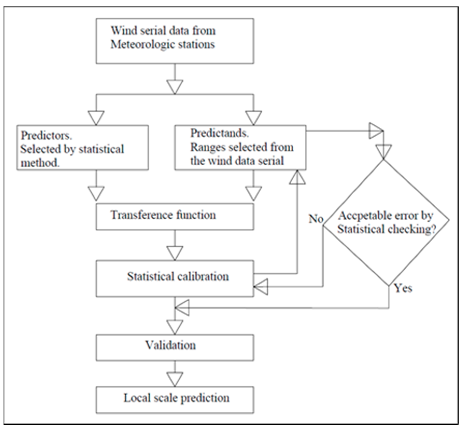
For that matter, a wind transfer equation based on regression and made from data series, terrain and atmosphere parameters could be posed for local scales. Figure 1 depicts the general idea for this wind data transference in reduced areas or at small scales.

So far, large-scale circulation models and the forecast from these for both large and regional scales have been widely developed. Representative examples of these include the wind field evaluation for surge storms in the Persian Gulf [3] and the achievement of wind speeds for a river basin in India from a GCM [4]. However, the question is to solve the impact of the climatic actions—in this case the wind—when it is acting over different local systems (harbours, shorelines, dunes, wind farms and beach geomorphology). This paper focuses on reviewing the state-of-the-art local-scale wind forecast models. Additionally, an attempt is made at identifying their advantages and disadvantages to clarify their scope and validity. Finally, we try to determine the characteristics that a wind transfer function should have to improve the deficiencies of the current models for forecasts in certain reduced areas, from wind data from nearby weather stations, and through this, a new line of research will be developed.

2. Methodology

The methodology is focused on the study of different papers to investigate the development of wind models and aims to select those that contribute applicable tools to get the parameters on a regional scale, not only from the global circulation models (GCMs) but also from meteorological stations near the study area. The investigation explores the different alternatives along with several ways to solve the problem depending on the area where the local wind was analysed. The point is to find which models have developed a wind transfer function on a scale of a few kilometres. For this purpose, the different downscaling applications normally used have firstly been identified. Table 1 provides a summary of them.

Table 1. Typology of the downscaling applications. Source: Adapted from Pielke and Wilby [5].

Purpose	Inputs to Regional Downscaling
Short-term prediction	Observed data and regional conditions analysis
Regional Simulation	Information from global reanalysis without considering initial conditions
Seasonal Prediction	Global model prediction from observed conditions
Climate Prediction	Multidecadal global prediction based on radiative forcing

Table 1. Typology of the downscaling applications. Source: Adapted from Pielke and Wilby [5].

Purpose	Inputs to Regional Downscaling
Short-term prediction	Observed data and regional conditions analysis
Regional Simulation	Information from global reanalysis without considering initial conditions
Seasonal Prediction	Global model prediction from observed conditions
Climate Prediction	Multidecadal global prediction based on radiative forcing

The downscaling techniques can be separated into two groups, which include, on the one hand, dynamic downscaling or DD [6], and on the other hand, statistical downscaling or SD [7]. A brief but accurate definition was extracted from the Geophysical Fluid Dynamics Laboratory web (https://www.gfdl.noaa.gov/): DD refers to the use of high-resolution regional simulations to dynamically extrapolate the effects of large-scale climate processes to regional or local scales of interest. In the so-called dynamic downscaling, high-resolution fields are obtained by nesting a regional climate model (RCM) within the GCM [8] or using a variable resolution GCM (the so-called stretching technique) [9]. SD encompasses the use of various statistics-based techniques to determine the relationships between large-scale climate patterns resolved by GCMs and the observed local climate responses. In statistical downscaling [10], the high-resolution predictands (surface variables) are obtained by applying previously identified relationships in the observed climate between these predictands and large-scale predictor fields to the outputs of the GCMs. Table 2 shows the advantages and disadvantages of both methods where some have been adapted from Climate Workspace (http://www.glisaclimate.org/) and other authors [11,12,13,14,15,16,17,18]:

Table 2. Advantages and disadvantages of statistical downscaling (SD) and dynamic downscaling (DD).

	Statistical Downscaling	Dynamic Downscaling
Advantages	Uses transfer functions (e.g., regression relationships) representing observed relationships between larger-scale atmospheric variables and local quantities [11].	Applied to obtain atmospheric information at a higher spatial resolution than that provided by global climate models, in particular for information on the influence of regional orographic characteristics [12]
	Statistically downscaled projections are relatively easy to produce because they do not require heavy computing resources. Due to the computation advantages mass ensembles of projections can be produced. Projections can also be downscaled to point-specific locations, however the data must be carefully interpreted at that scale. The results can be compared to observations for a historical time period.	Is based on regional climate models (usually just the atmospheric part) that have a finer horizontal grid resolution of surface features such as terrain [13]. The benefits of dynamical downscaling with respect to a more realistic representation of winds over a complex terrain were documented e.g., [14].
Disadvantages	Two major disadvantages exist: Local, small-scale dynamics and climate feedbacks are not simulated. Assumptions of stationarity between the large- and small-scale dynamics are made to downscale future projections. The GCMs cannot simulate weather and climate processes at scales smaller than their grid spacing, and statistically downscaled data does not add information at the smaller scale. Statistically downscaled data can only reflect the information in the observations onto the projections.	Dynamical downscaling is affected by different sources of uncertainty. The most important are uncertainties in the parameterisation of physical processes and in the numerical formulation of the Regional Climate Models (RCMs), sensitivity to the initial conditions or to boundary conditions, and uncertainty due to the internal variability generated within the model domain [15].
		The accuracy of the DD is insufficient or occasionally inferior to the SD when verifying the downscaling of a present-day analysis against observations [16].
		Another issue from the numerical weather prediction model (NWP) points of view were developed by Foley et al. [17] and Hong and Kanamitsu [18].

Table 2. Advantages and disadvantages of statistical downscaling (SD) and dynamic downscaling (DD).

	Statistical Downscaling	Dynamic Downscaling
Advantages	Uses transfer functions (e.g., regression relationships) representing observed relationships between larger-scale atmospheric variables and local quantities [11].	Applied to obtain atmospheric information at a higher spatial resolution than that provided by global climate models, in particular for information on the influence of regional orographic characteristics [12]
	Statistically downscaled projections are relatively easy to produce because they do not require heavy computing resources. Due to the computation advantages mass ensembles of projections can be produced. Projections can also be downscaled to point-specific locations, however the data must be carefully interpreted at that scale. The results can be compared to observations for a historical time period.	Is based on regional climate models (usually just the atmospheric part) that have a finer horizontal grid resolution of surface features such as terrain [13]. The benefits of dynamical downscaling with respect to a more realistic representation of winds over a complex terrain were documented e.g., [14].
Disadvantages	Two major disadvantages exist: Local, small-scale dynamics and climate feedbacks are not simulated. Assumptions of stationarity between the large- and small-scale dynamics are made to downscale future projections. The GCMs cannot simulate weather and climate processes at scales smaller than their grid spacing, and statistically downscaled data does not add information at the smaller scale. Statistically downscaled data can only reflect the information in the observations onto the projections.	Dynamical downscaling is affected by different sources of uncertainty. The most important are uncertainties in the parameterisation of physical processes and in the numerical formulation of the Regional Climate Models (RCMs), sensitivity to the initial conditions or to boundary conditions, and uncertainty due to the internal variability generated within the model domain [15].
		The accuracy of the DD is insufficient or occasionally inferior to the SD when verifying the downscaling of a present-day analysis against observations [16].
		Another issue from the numerical weather prediction model (NWP) points of view were developed by Foley et al. [17] and Hong and Kanamitsu [18].

The several reviewed papers lead to the conclusion that SD is the technique to be applied to reduced areas. The main reasons are its feasibility and ability to diagnose at local scales, as well as performing over different time scales [19]. The dynamic downscaling and its different types [13] are still not the final solution, such as a way to predict wind in near field, because of the different aspects such as the atmospheric/oceanic boundary conditions, circulations, or the limited spatial resolution [5]. Additionally, DD is practically the same as GCMs but with a higher resolution. This implies the DD is computationally intensive and requires large volumes of data, as well as a high level of experience to implement and interpret the results. Devis et al. [20], already delved into this point after making a comparison between dynamical and statistical downscaling, and the main conclusion found was that dynamical downscaling can be used for regional climatic models between approximately 20 and 50 km, with the boundary conditions provided by a GCM. The statistical downscaling develops important transference functions. These functions relate the great-scale GCM models, with the near field. The main advantage over the dynamical downscaling is the relative ease of use and application in assembly with GCM.

The experience from Puertos del Estado (the state-owned Spanish port system, http://www.puertos.es/es-es) is one of the precedent cases to the achievement of climatic parameters in the near field. It is focused on wave forecasting on the coastal shoreline [21]. The aim of this investigation was to find the waves in the continental shelf as data coming from a GCM, such as the WAM model [22] and SWAN model [23], or SMC [24]. These models predict the waves in coasts, lakes, and estuaries for a certain wind pattern and this propagation can be used in many different fields, for example for the gradation of sand beaches such as that developed by Bernabeu et al. [25]. The problem was solved for Puertos del Estado by dividing the system into two steps: one at an oceanic scale and another at a local scale nested with the first one and introducing a set of applications to solve the problem in the specific port area. Another experience was carried out by Machado et al. [26] on Deception Island, where the model was validated by comparing the simulation results against data collected in several stations inside the domain. The idea may be similar but is applied to the wind, also considering how to proceed from meteorological station data series whilst taking advantages from previous conducted investigations. Therefore, the methodology consists of selecting the research that contributes applicable findings. These will be developed in a future line of research.

3. Results and Discussion

This section has been structured into five different subsections for the SD. The idea is to go down from the typical models to reach the transfer functions passing through the used mathematical expressions, approaches, and common probability density functions.

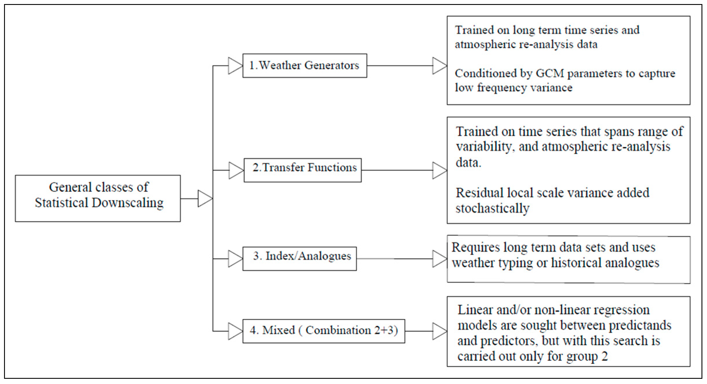
Firstly, Figure 2 summarises the techniques traditionally used for statistical downscaling.

Figure 2. SD techniques classification. Source: Adapted from Hewitson et al. [27].

Figure 2. SD techniques classification. Source: Adapted from Hewitson et al. [27].

3.1. Statistical Downscaling Methods Used

The statistical downscaling is based on regression relationships. Basically, these methods are empirical relationships linking large-scale atmospheric variables (predictors) with some local-scale variables of interest (predictands) [28]. This could be the way to solve the issues above indicated but it is not clear so far. Following this, a revision of the latest works carried out during the last 15 years is undertaken, remarking on the possible articles and papers that, where exposed, expose the current state of this matter.

Table 3. Different SD methods. Advantages and disadvantages. Source: Adapted from Sunyer et al. [29].

SD Method	Advantages	Disadvantages
Bias Correction of: Mean/ Mean and Variance. (T.G. Masaryk Water Research Institute) Quantile Mapping. (NVE)	Easy to apply and little computer time required. Accounts for different corrections in different time windows. Allows for distinct corrections between mean and variance. Distinction between corrections in mean and extreme values. No theorical distribution is assumed.	It only corrects the mean values of RCMs. The non-linear transformation may lead to unexpectedly large values. The autocorrelation for RCMs is not corrected, but is affected by the bias correction approach. The correction of the upper is based on relatively few values (empirical distribution based). The same correction is applied for all the seasons. The autocorrelation for RCMs is not corrected, but it is affected by the bias correction approach.
Expanded downscaling. (U. Potsdam)	Generates realistic weather consistent with large-scale atmospheric patterns. Can employ the full range of predictor variables. Preserves co-variability between the predictands	High demand for climate model accuracy; systematic biases can cause large errors. Requires large computation time and data preparation. No fully objective way of selecting the predictors
Change factor of: Mean/ Mean and Variance. (DHI, DTU) Quantile Mapping. (DTU) Quantile Perturbation. (KU Leuven)	Easy to apply and little computer time required. Accounts for different corrections in different time windows Distinction between corrections in mean and extreme values. No theorical distribution is assumed. Changes in the frequency of values are accounted for	Only accounts for changes in mean values. The autocorrelation of values may be disturbed. The non-linear transformation may lead to unexpectedly large values. The changes in the tails are based on relatively few values

provides a summary of the different statistical downscaling methods [29]:

Another area of knowledge, where the wind forecast plays an important role, is wind power generation, not only from the power generation point of view, but from the design of the marine civil works such as offshore wind civil foundations [30]. Due to the random features of the wind, the need to have an accurate forecast is increasing constantly. In this sense, the different statistical wind forecasts have been discussed, focused on the forecast from the large to the regional scale, especially during downscaling.

3.2. Common Mathematical Expressions for Statistical Wind Downscaling

The downscaling is going to be discussed as a statistical technique in relation to the mathematical expressions used. It needs a comfortable mathematical expression to work, but the range of covered values must also be as wide as possible. Additionally, maximum flexibility with the data is necessary. In this sense, the Weibull expression plays an important role for its good fit of the peaks values [31].

One of the problems posed is to obtain a tractable expression for the wind probability density functions, and based on this, the orthogonal polynomials [32] could be an option (perpendicular, or at right angles to each other). The research sought to determine if simple expressions could be used from nonparametric kernels (a kernel is a weighting function used in non-parametric estimation techniques), to approximate wind probabilistic density functions (wind PDF) for those what have a deficient fitting, like 2 parameter-Weibull functions. The mathematical expression for this probability density function (PDF) of a 2 parameter Weibull distribution for positive wind values (V ≥ 0) can be expressed as

$$f\left(V\right) = \frac{\beta }{\alpha }{\left(\frac{V}{\alpha }\right)}^{\beta -1}{e}^{(-{\left(\frac{V}{\alpha }\right)}^{\beta })}$$

(1)

where α and β are the scale and shape parameters, respectively. They can be obtained through the maximum likelihood estimation. The Weibull shape parameter, β, is also known as the Weibull slope. This is because the value of β is equal to the slope of the line in a probability plot. A change in the scale parameter, α, has the same effect on the distribution as a change in the abscissa scale. Increasing the value of α while holding β constant has the effect of stretching out the wind PDF.

A robust estimation of traditional Weibull functions was also achieved. Between the nonparametric regression techniques, the Kernel interpolation turned out to be flexible and useful but not simple, especially for downscaling from climatic models or wind turbine applications because a tractable analytic expression cannot be obtained from the Kernel method as the number of terms in kernel expressions equals the number of data points used in the fit [32]. Other important points were discovered; the Gauss–Hermite expansions for wind PDF could be set forth as per scale parameters [32], or the settings in a Gauss–Kernel interpolation function could be used as fitting standards. One remarkable conclusion was that there will be always an expansion orthogonal polynomial which improves the wind PDF fittings for a Weibull expression. In this field, the Gram–Schmidt method is a worthy option to build useful fittings for the wind velocity histograms.

3.3. Statistical Downscaling Approaches for Local Forecasts

As stated in the previous paragraphs, the mathematical statistics are the base for this research and the regression study for the wind PDF is the technique used. Bedia et al. [33] indicated that the application of SD techniques to GCMs consists of two phases. In the training phase, the model parameters are fitted to data and cross-validated using a representative historical period (i.e., a few decades) with existing predictor and predictand data. In the second, the downscaling phase, the predictors given by the GCM outputs are plugged into the models to obtain the corresponding locally downscaled values for the predictands. According to the approach followed in the training phase, the different SD techniques can be classified into two categories [34]: Perfect Prognosis (PP) and Model Output Statistics (MOS).

In the PP approach, the statistical model is calibrated using observational data for both the predictands and predictors [28]. In this approach, the predictors and predictands keep the correspondence day to day [33], while in the MOS approach the predictors are taken from the same GCM for both the training and downscaling phases. The MOS methods typically work with the (locally interpolated) forecasts and observations of the variable of interest (a single predictor) [33]. Previous investigations have focused on the study of the regression from circulation models [20], such as the ECHAM5 model (Circulation Models of Max Planck Society). As indicated, most of PP and MOS techniques are based on the statistical downscaling from serial data. This could provide a fitting procedure, for example, in the case of dune movement [35], or when long data series from meteorological stations near the dunes (around 10 km) are used, like in the case of Valdevaqueros Dune, to fine-tune the effects of aeolian transport [36] or establish wind conditions for the use of a remotely piloted aircraft system (RPAS) in the Beach levelling [37].

Other considerations regarding the PP approach [28] were that the variables directly influenced by the statistical model and orography are not suitable predictors in this approach. Therefore, one of the large tasks for these methods is the screening of appropriate combinations of predictors for each predictand and region of study.

For the MOS, the main problem was the lack of daily correspondence between forecasts and observations over longer time scales. This was satisfactorily solved by the reanalysis-nudged GCM [38], but the most important issue was the avoid stationary-related problems, which can be solved by the bias correction techniques conditioned on weather types [39]. Additionally, and considering the time scale, it was demonstrated that the GCM cannot be used directly for the lineal relation between predictors and predictands because the correlation between monthly or hourly observations does not exit. For this purpose, it is compulsory to assemble a transference function between scales inside the GCM. These investigations above indicated helped to show that statistical downscaling is valid in both the short and the long term in wind forecast. Focused on the short term, statistical downscaling could be much improved through a band time discrimination, especially when there was a marked seasonal effect between daytime and nighttime hours in the data series. Lastly, the research undertaken in Cabauw (Utrecht) [20] used the ECHAM5 model to apply the 2 parameter Weibull function to the results. This function fitted well for diurnal winds, but also revealed a great skewness in night spectra with variations of the shape parameters considering the influence of the atmosphere in the wind equation depending on the site height.

3.4. Common PDF Distributions Used in SD to Develop Transference Equations

There is no unique method for developing a transference equation from statistical downscaling but a well-structured methodology could be based on Gamma functions [40]. For Kirchmeier et al. [40], whose study was in The Great Lakes Region (USA), the Gamma function was established with simple functions, to calculate the relation between the mean and standard deviation of the shape and scale parameters. A considerable accuracy increase was achieved where the data was hourly instead of monthly. The summarised methodology consisted of choosing a probabilistic density function from the types: Gumbel (type I), Fréchet (type II), or Weibull (type III). Once the predictors were selected and fitted as per a statistical process, the obtained values had to be inside a confidence range. Important points were to perform an analysis of the observed extreme values and to study the spatial and temporal variability and how it affects the model and its equations. Some papers [41] established a way to deal with this double issue. Firstly, the temporal variability is solved directly with statistical downscaling. Secondly, the spatial variability can be solved with the Wind Profile Power Law model [42]. This last model leads to the introduction of a new question, the wind profiles. The wind profile models, and their forecast have been developed a lot in the wind power field. The classification of the wind models can be as follows [43]:

Physical models: physical models use physical considerations, such as terrains, obstacles, pressure, and temperatures, to estimate the future wind speed [44]. Examples of these are the numerical weather prediction modes (NWP).

Statistical and computational models: basically, statistical methods use the previous history of wind data to perform a forecast over the next few hours, they are good for short periods of time. The disadvantage of this method is that forecast error increases as time forecasting increases, i.e., statistical time series and methods of neural networks are primarily intended for short-term forecasts [45].

Hybrid models: usually, the combination of different approaches, such as physical and statistical approaches, models combining short and medium term, etc., is commonly referred to as a mixed or hybrid model approach [46].

According to Ehlers [47], these models have the main particularity of temporal data series treatment and the main disadvantages are related to the difficulty of analysing correlated observations and their temporal orders. Additional issues are generated by the trends, seasonal, or cyclical variations, and the sequential nature of the missing data. These points require complex and specific resolution techniques which become complicated in models.

3.5. Transference Equations in Statistical Downscaling

The transference equations in the wind fields will be discussed in the following section. The question here is to find an efficient and profitable alternative for introducing data from the microscale (9–10 km) into mesoscale models (from 10 to 2000 km), such as computational fluid dynamics (CFD) or NWP models [48]. The aim of Barcons et al. [48] was to solve the issues on a local scale where the terrains were very rough (mountain or complex orography). The authors proposed a methodology where the first step was to build a series of 2D terrain grids to which the downscaled winds were applied. After that, these grids were decomposed or segmented to be referenced to the mesoscale. The connections between the microscale and mesoscale were warranted by lineal interpolation. The overlapping regions were deeply developed to obtain a smooth transition between the micro and mesoscales due to the small variations in wind direction on the mesoscale. Finally, the transfer functions were applied to scale the microscale wind velocity at each point of the 2D planes.

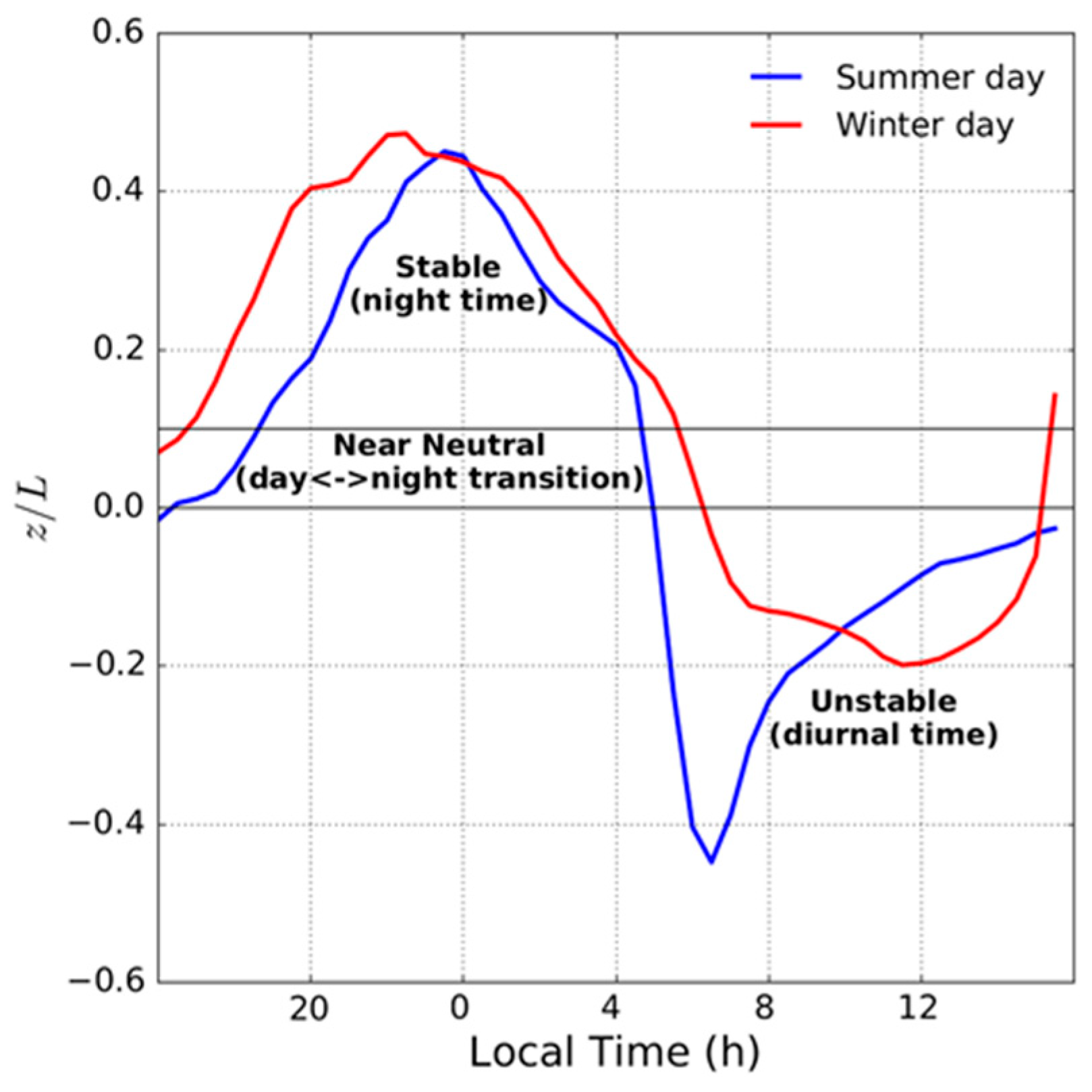
Apart from the local terrain features, the relation between wind intensity and atmospheric stability is another aspect that needs to be considered. Barcons et al. [48] proposed the use of the Obukhov length (L) from the Monin–Obukhov similarity theory, used to describe the effects of buoyancy on turbulent flows, particularly in the lower tenth of the atmospheric boundary layer, and the layer at height (Z). An atmospheric stability description can be established based on these two factors:

• Z/L > 0.1 stable;
• 0.1 ≥ Z/L ≥ 0 near natural;
• Z/L < 0.1 unstable.

Z/L is the dimensionless stability parameter, which varies depending on the season, as shown in the following chart (Figure 3).

The influence of the effects of wind acceleration due to the presence of topography, or the wind’s decrease and turning into valleys and channelling areas, are factors to be considered in the regional analysis. The downscaling results did not show improvement during unstable regimes and during low wind speeds, where thermal effects prevailed. This can be explained by the assumption of neutral stability in the previously calculated fields and evidence of the need to incorporate the thermal effects of the diurnal cycle in the simulations.

Another factor influencing wind acceleration is the Coriolis force. This affects the wind profile by introducing a rotation with a height and a non-logarithmic wind profile above the surface layer (around 100 m). Furthermore, additional issues appear when the applied mixing length limitation assumes the values of the homogeneously flat terrain.

3.6. Weibull Distribution for SD Transference Equations

The main points to be considered for wind forecast at a local scale have been presented. We now focus on the models that have developed a transference equation from the Weibull distribution. There is a recent method that uses the temporal scales to downscale the wind speed probability distribution to a fine scale without using other variables [49]. For the development of the method, a maximum temporal scale of 4 weeks and wind observation of 10 min intervals were fixed. This was due to the large temporal scales that probably led to bad results for wind statisticians. The chosen temporal scales ranged from a maximum of a day and a minimum of an hour. After this fitting, although any probability distribution could be used, the Weibull distribution was selected and its parameters were estimated, and finally the wind probabilities’ distribution was fixed on a small temporal scale.

Another method was developed in the Persian Gulf Area, which proposes a means of statistical downscaling where the Weibull parameters are used as predictands [50]. This way of addressing the problem had already been considered by Pryor and Barthelmie [51] for wind data from 85 weather stations located in the east of the USA, and also by Chang et al. for the Taiwan Strait [52]; a multiple linear regression method for the 2 Weibull parameters and the mean and standard deviation of the relative vorticity were developed. These methods achieved statistical downscaling based on the Weibull distribution from GCMs.

The previous method found that the statistical downscaling for the Weibull distribution and its parameters achieved a good performance for the peak values and it was noticed that the wind direction can be modified automatically using the downscaling approach for wind components from GCMs.

Aligned with the previous method, Alizadeh et al. [3] followed the investigation and, in the same way, used GCMs from the European centre for medium-range weather forecasts (ECMWF). For the wind downscaling based on the Weibull distribution technique, the Weibull parameters were modified to obtain reliable future forecasts (3). The authors pointed out that these previous models, which had used the inverse distance weighting, did not consider the heterogeneity and the spatial variation in areas with high wind speed gradients. Additionally, they corroborated that the Weibull-based techniques outperform the accuracy of the existing statistical downscaling techniques.

4. Future Lines of Research

The different methods revised each have different advantages and disadvantages, and one best option cannot be established. The main issues include that

• GCMs cannot be used directly to establish a lineal relation between predictors and predictands due to the lack of correlation between the time terms for the large scale and local scale, implying that a transference function must be assembled in the GCM.
• Regarding the wind models, the NWP are only valid at the mesoscale and large scale; the statistical models have difficulties forecasting with large data series or when the forecast times are so long.
• Additionally, the SD techniques used for the local scale, such as PP or MOS, have issues that imply an adequate screening of the predictors for each predictand or stationarity problems.
• Lastly, the current transference equations are disturbed by the orography and, particularly, terrain accidents, thermal effects, Coriolis force, or the mixing length model used.

Future work must investigate if only one equation is possible independent of the site features or if it should be discretized per type terrain and elevation. Two important points are clear: the hourly discretisation helps improve the SD, and the Weibull distribution is proven as a good fit for any wind model. This, along with understanding how each author tried to solve the indicated problems, could be the baseline of future research. So, a new investigation could define a transference equation based on the Weibull distribution to improve or remove the disadvantages exposed here. Further questions will include how to nest the equation or equations to ensure the correct transference with the wind models. This also would be useful for specific local applications that infer the wind forecast from meteorological stations located a few kilometres away from the studied place.

5. Conclusions

As indicated above, regional downscaling is focused on local data (predictands) achievements from the large scale, such as from GCMs (predictors). Neither of the latest researched models have solved these questions properly, especially due to problems in obtaining accurate forecasts when there is a high wind gradient. The large number of consulted papers shows there is not a single methodology or procedure to extract the most accurate method, and that there is an important dependence on the area, its topography features, and the atmosphere interactions according to the altitude.

Different comparatives studies conducted in different regions have demonstrated that there is no single statistical downscaling approach that is optimal for all regions and applications. However, its general advantages include its ease of application, that it makes a distinction between the corrections for the mean, variance, and extrema values, and it can employ a full range of predictor variables, accounting for the frequency changes of values.

The main disadvantage of SD is the problem of stationarity in the context of climate change, and since the season features change, this can lead to the predictor–predictands relationship detected in the present not being applied in the future. Other disadvantages include the limitations of GCMs, and finally the statistical methodology must be non-linear enough for a strong non-linear relationship between the predictors and predictands in local climatology to be maintained.

Another remarkable point is that local serial data from the weather stations have been used for the calibration of the results, but the extensive consulted bibliography does not reveal a method only based directly on these stations for forecasts in the local extension range of 10–50 km. It is probably important to investigate spatially reduced areas from the data offered by meteorological stations near the studied area. All of these questions can lead to a new field of research considering the important achievements so far. This new line of work could be focused on transference equations from meteorological stations’ data, including the atmospheric and terrain parameters, whilst connecting these equations to the mesoscale models.

References

- Huebener, H.; Cubasch, U.; Langematz, U.; Spangehl, T.; Niehörster, F.; Fast, I.; Kunze, M. Ensemble climate simulations using a fully coupled ocean–troposphere–stratosphere general circulation model. Philos. Trans. R. Soc. A Math. Phys. Eng. Sci. 2007, 365, 2089–2101. [Google Scholar] [CrossRef] [PubMed]
- Schoof, J.T. Statistical Downscaling in Climatology. Geogr. Compass 2013, 7, 249–265. [Google Scholar] [CrossRef] [Green Version]
- Alizadeh, M.J.; Kavianpour, M.R.; Kamranzad, B.; Etemad-Shahidi, A. A distributed wind downscaling technique for wave climate modeling under future scenarios. Ocean Model. 2020, 145, 101513. [Google Scholar] [CrossRef]
- Anandhi, A.; Srinivas, V.V.; Kumar, D.N.; Nanjundiah, R.S. Role of predictors in downscaling surface temperature to river basin in India for IPCC SRES scenarios using support vector machine. Int. J. Climatol. 2009, 29, 583–603. [Google Scholar] [CrossRef]
- Pielke, R.A.; Wilby, R.L. Regional climate downscaling: What’s the point? Eos Trans. Am. Geophys. Union 2012, 93, 52–53. [Google Scholar] [CrossRef]
- Giorgi, F.; Francisco, R. Uncertainties in regional climate change prediction: A regional analysis of ensemble simulations with the HADCM2 coupled AOGCM. Clim. Dyn. 2000, 16, 169–182. [Google Scholar] [CrossRef]
- Wilby, R.L.; Wedgbrow, C.S.; Fox, H.R. Seasonal predictability of the summer hydrometeorology of the River Thames, UK. J. Hydrol. 2004, 295, 1–16. [Google Scholar] [CrossRef]
- Christensen, J.H.; Carter, T.R.; Rummukainen, M.; Amanatidis, G. Evaluating the performance and utility of regional climate models: The PRUDENCE project. Clim. Chang. 2007, 81, 1–6. [Google Scholar] [CrossRef]
- Giorgi, F.; Brodeur, C.S.; Bates, G.T. Regional Climate Change Scenarios over the United States Produced with a Nested Regional Climate Model. J. Clim. 1994, 7, 375–399. [Google Scholar] [CrossRef] [Green Version]
- Imbert, A.; Benestad, R.E. An improvement of analog model strategy for more reliable local climate change scenarios. Theor. Appl. Clim. 2005, 82, 245–255. [Google Scholar] [CrossRef]
- Group, T.; Support, S.; Assessment, C.; Panel, I.; Change, C. General Guidelines on the Use of Scenario Data for Climate Impact and Adaptation Assessment; Finnish Environmental Institute: Helsinki, Finland, 2007.
- Donat, M.; Leckebusch, G.C.; Wild, S.; Ulbrich, U. Benefits and limitations of regional multi-model ensembles for storm loss estimations. Clim. Res. 2010, 44, 211–225. [Google Scholar] [CrossRef] [Green Version]
- Castro, C.L.; Pielke, R.A.; Leoncini, G. Dynamical downscaling: Assessment of value retained and added using the Regional Atmopsheric Modeling System (RAMS). J. Geophys. Res. D Atmos. 2005. [Google Scholar] [CrossRef]
- Žagar, N.; Zagar, M.; Cedilnik, J.; Gregoric, G.; Rakovec, J. Validation of mesoscale low-level winds obtained by dynamical downscaling of ERA40 over complex terrain. Tellus A Dyn. Meteorol. Oceanogr. 2006, 58, 445–455. [Google Scholar] [CrossRef]
- Von Storch, J.-S. Interdecadal variability in a global coupled model. Tellus A 1994, 46, 419–432. [Google Scholar] [CrossRef]
- Murphy, J. An Evaluation of Statistical and Dynamical Techniques for Downscaling Local Climate. J. Clim. 1999, 12, 2256–2284. [Google Scholar] [CrossRef]
- Foley, A.M.; Leahy, P.G.; Marvuglia, A.; McKeogh, E.J. Current methods and advances in forecasting of wind power generation. Renew. Energy 2012, 37, 1–8. [Google Scholar] [CrossRef] [Green Version]
- Hong, S.-Y.; Kanamitsu, M. Dynamical downscaling: Fundamental issues from an NWP point of view and recommendations. Asia-Pacific J. Atmos. Sci. 2014, 50, 83–104. [Google Scholar] [CrossRef]
- Wilby, R.; Wigley, T. Downscaling general circulation model output: A review of methods and limitations. Prog. Phys. Geogr. Earth Environ. 1997, 21, 530–548. [Google Scholar] [CrossRef]
- Devis, A.; Van Lipzig, N.P.M.; Demuzere, M. A new statistical approach to downscale wind speed distributions at a site in northern Europe. J. Geophys. Res. Atmos. 2013, 118, 2272–2283. [Google Scholar] [CrossRef] [Green Version]
- Gómez Lahoz, M.; Albiach, J.C.C. Wave forecasting at the Spanish coasts. J. Atmos. Ocean Sci. 2005, 10, 389–405. [Google Scholar] [CrossRef]
- Group, T.W. The WAM Model—A Third Generation Ocean Wave Prediction Model. J. Phys. Oceanogr. 1988, 18, 1775–1810. [Google Scholar] [CrossRef] [Green Version]
- Booij, N.; Ris, R.C.; Holthuijsen, L.H. A third-generation wave model for coastal regions: 1. Model description and validation. J. Geophys. Res. Space Phys. 1999, 104, 7649–7666. [Google Scholar] [CrossRef] [Green Version]
- Gonzalez, M.; Medina, R.; Gonzalez-Ondina, J.; Osorio, A.F.; Méndez, F.; Garcia, E. An integrated coastal modeling system for analyzing beach processes and beach restoration projects, SMC. Comput. Geosci. 2007, 33, 916–931. [Google Scholar] [CrossRef]
- Bernabeu, A.M.; Lersundi-Kanpistegi, A.V.; Vilas, F. Gradation from oceanic to estuarine beaches in a ría environment: A case study in the Ría de Vigo. Estuarine Coast. Shelf Sci. 2012, 102-103, 60–69. [Google Scholar] [CrossRef]
- Machado, J.A.T.; Baleanu, D.; Luo, A.C.J.; Vidal, J.; Berrocoso, M.; Jigena, B. Hydrodynamic Modeling of Port Foster, Deception Island (Antarctica). In Nonlinear and Complex Dynamics; Springer: London, UK, 2011. [Google Scholar]
- Hewitson, B.C.; Daron, J.; Crane, R.G.; Zermoglio, M.F.; Jack, C. Interrogating empirical-statistical downscaling. Clim. Chang. 2014, 122, 539–554. [Google Scholar] [CrossRef] [Green Version]
- Gutiérrez, J.M.; San-Martín, D.; Brands, S.; Manzanas, R.; Herrera, S. Reassessing Statistical Downscaling Techniques for Their Robust Application under Climate Change Conditions. J. Clim. 2013, 26, 171–188. [Google Scholar] [CrossRef] [Green Version]
- Sunyer, M.A.; Hundecha, Y.; Lawrence, D.; Madsen, H.; Willems, P.; Martinkova, M.; Vormoor, K.; Bürger, G.; Hanel, M.; Kriaučiūnienė, J.; et al. Inter-comparison of statistical downscaling methods for projection of extreme precipitation in Europe. Hydrol. Earth Syst. Sci. 2015, 19, 1827–1847. [Google Scholar] [CrossRef] [Green Version]
- Negro, V.; López-Gutiérrez, J.-S.; Esteban, M.D.; Alberdi, P.; Imaz, M.; Serraclara, J.-M. Monopiles in offshore wind: Preliminary estimate of main dimensions. Ocean Eng. 2017, 133, 253–261. [Google Scholar] [CrossRef]
- Pinto, H.; Amini, A.; Peña, Á.; Moraga, P.; Valenzuela, M. Fatigue and damage accumulation in open cell aluminium foams. Fatigue Fract. Eng. Mater Struct. 2018, 41, 483–493. [Google Scholar] [CrossRef]
- Morrissey, M.L.; Greene, J.S. Tractable Analytic Expressions for the Wind Speed Probability Density Functions Using Expansions of Orthogonal Polynomials. J. Appl. Meteorol. Clim. 2012, 51, 1310–1320. [Google Scholar] [CrossRef]
- Bedia, J.; Baño-Medina, J.; Legasa, M.N.; Iturbide, M.; Manzanas, R.; Herrera, S.; Casanueva, A.; San-Martín, D.; Cofiño, A.S.; Gutiérrez, J.M. Statistical downscaling with the downscaleR package (v3.1.0): Contribution to the VALUE intercomparison experiment. Geosci. Model Dev. 2020, 13, 1711–1735. [Google Scholar] [CrossRef] [Green Version]
- Marzban, C.; Sandgathe, S.; Kalnay, E. MOS, Perfect Prog, and Reanalysis. Mon. Weather. Rev. 2006, 134, 657–663. [Google Scholar] [CrossRef]
- Rodríguez Santalla, I.; Sánchez García, M.J.; Montoya Montes, I.; Gómez Ortiz, D.; Martín Crespo, T.; Serra Raventos, J. Internal structure of the aeolian sand dunes of El Fangar spit, Ebro Delta (Tarragona, Spain). Geomorphology 2009, 104, 238–252. [Google Scholar] [CrossRef]
- Martell-Dubois, R.; Mendoza-Baldwin, E.; Mariño-Tapia, I.; Silva-Casarín, R.; Escalante-Mancera, E. Impactos de corto plazo del huracán Dean sobre la morfología de la playa de Cancún, México. Technol. Ciencias Agua 2012, 3, 89–111. [Google Scholar]
- Contreras-De-Villar, F.; García, F.J.; Muñoz-Perez, J.J.; Contreras-De-Villar, A.; Ruiz-Ortiz, V.; Lopez, P.; Garcia-López, S.; Jigena, B. Beach Leveling Using a Remotely Piloted Aircraft System (RPAS): Problems and Solutions. J. Mar. Sci. Eng. 2020, 9, 19. [Google Scholar] [CrossRef]
- Eden, J.M.; Widmann, M.; Grawe, D.; Rast, S. Skill, Correction, and Downscaling of GCM-Simulated Precipitation. J. Clim. 2012, 25, 3970–3984. [Google Scholar] [CrossRef] [Green Version]
- Wetterhall, F.; Pappenberger, F.; He, Y.; Freer, J.; Cloke, H.L. Conditioning model output statistics of regional climate model precipitation on circulation patterns. Nonlinear Process. Geophys. 2012, 19, 623–633. [Google Scholar] [CrossRef] [Green Version]
- Kirchmeier, M.C.; Lorenz, D.J.; Vimont, D.J. Statistical Downscaling of Daily Wind Speed Variations. J. Appl. Meteorol. Clim. 2014, 53, 660–675. [Google Scholar] [CrossRef]
- Kirchner-Bossi, N.; García-Herrera, R.; Prieto, L.; Trigo, R.M. A long-term perspective of wind power output variability. Int. J. Clim. 2014, 35, 2635–2646. [Google Scholar] [CrossRef] [Green Version]
- Counihan, J. Adiabatic atmospheric boundary layers: A review and analysis of data from the period 1880–1972. Atmos. Environ. (1967) 1975, 9, 871–905. [Google Scholar] [CrossRef]
- De Alencar, D.B.; De Mattos Affonso, C.; De Oliveira, R.C.L.; Rodríguez, J.L.M.; Leite, J.C.; Filho, J.C.R. Different Models for Forecasting Wind Power Generation: Case Study. Energies 2017, 10, 1976. [Google Scholar] [CrossRef] [Green Version]
- Lei, M.; Shiyan, L.; Chuanwen, J.; Hongling, L.; Yan, Z. A review on the forecasting of wind speed and generated power. Renew. Sustain. Energy Rev. 2009, 13, 915–920. [Google Scholar] [CrossRef]
- Chang, W.-Y. A Literature Review of Wind Forecasting Methods. J. Power Energy Eng. 2014, 2, 161–168. [Google Scholar] [CrossRef]
- Soman, S.S.; Zareipour, H.; Malik, O.P.; Mandal, P. A review of wind power and wind speed forecasting methods with different time horizons. In Proceedings of the North American Power Symposium 2010, Arlington, TX, USA, 26–28 September 2010; pp. 1–8. [Google Scholar]
- Ehlers, R.S. Análise de séries Temporais, 5th ed.; CAMPUS: Parana, Brasil, 2009; p. 118. [Google Scholar]
- Barcons, J.; Avila, M.; Folch, A. A wind field downscaling strategy based on domain segmentation and transfer functions. Wind. Energy 2018, 21, 409–425. [Google Scholar] [CrossRef] [Green Version]
- Shin, J.-Y.; Jeong, C.; Heo, J.-H. A Novel Statistical Method to Temporally Downscale Wind Speed Weibull Distribution Using Scaling Property. Energies 2018, 11, 633. [Google Scholar] [CrossRef] [Green Version]
- Alizadeh, M.J.; Kavianpour, M.R.; Kamranzad, B.; Etemad-Shahidi, A. A Weibull Distribution Based Technique for Downscaling of Climatic Wind Field. Asia-Pac. J. Atmos. Sci. 2019, 55, 685–700. [Google Scholar] [CrossRef]
- Pryor, S.C.; Barthelmie, R.J. Hybrid downscaling of wind climates over the eastern USA. Environ. Res. Lett. 2014, 9, 024013. [Google Scholar] [CrossRef] [Green Version]
- Chang, T.-J.; Chen, C.-L.; Tu, Y.-L.; Yeh, H.-T.; Wu, Y.-T. Evaluation of the climate change impact on wind resources in Taiwan Strait. Energy Convers. Manag. 2015, 95, 435–445. [Google Scholar] [CrossRef]