Near Real-Time Monitoring of Significant Sea Wave Height through Microseism Recordings: Analysis of an Exceptional Sea Storm Event

Abstract

Microseisms are used to estimate significant sea wave heights (H_s) in different parts of the world and also during extreme events (e.g., typhoons and hurricanes), as they are generated by the effect of sea waves on the sea bottom and are strictly related to the wave height. On 29 October 2018, an exceptional sea storm event (the Adrian storm) occurred in the Ligurian Sea (NW Mediterranean Sea), producing severe damage to coastal constructions and infrastructures. However, the microseism measured at seismic stations located near the coast did not show equivalent high energy, thus resulting in a severe underestimation of the H_s predicted. In the present study, the Adrian storm was compared to other sea storms that have occurred in the Ligurian Sea in recent decades. The aim of this paper is to statistically examine the distinctive peculiarities of the Adrian storm in order to find new parameters to insert in the empirical models used in the procedure recently implemented for monitoring of H_s through microseism recordings in the Ligurian Sea, improving the effectiveness in H_s estimates in cases of extreme events that do not produce high-energy microseisms. The results show that the additional parameters to be taken into account into the predictive model are the atmospheric pressure gradient and the wind intensity. A correction term is finally proposed and applied to the predictive model to significantly reduce the H_s underestimation.

1. Introduction

Sea wave height is one of the most relevant sea parameters to the monitoring and protection of coastal areas and to mitigation of marine risk associated with the occurrence of strong sea storm events. The study of the wave characteristics, such as wave period, wavelength, significant wave height, and return period of sea storm, is essential for the design of offshore and coastal infrastructures, such as oil platforms, wind farms, breakwaters and artificial reefs, and for their conservation [1,2]. Due to the impact of sea waves on economic activities, a great effort has been made in the last decades to develop methods for direct sea wave height measurements using wave buoys. Nonetheless, wave buoys are typically very expensive and problematic, especially regarding their installation and maintenance. Moreover, they usually provide discontinuous data (e.g., due to temporary damage) with poor spatial resolution (due to the low density of monitoring stations in sea areas). Most common alternative methods are based on numerical modelling [3,4], remote sensing [5,6,7], coastal radars [8,9], and microseism recordings [10,11,12,13,14,15].

Microseisms are produced by the pressure exerted by sea waves on the sea floor and propagate in the surface layer of seabed for hundreds of kilometres thanks to their low frequency content, which typically ranges between 0.05 and 0.5 Hz. Microseisms are classically divided into primary and secondary microseisms. Primary microseisms cover the same frequency range of ocean swells, between 0.05 and 0.1 Hz, and are generated by pressure variation induced by sea waves on the seabed in coastal areas. The secondary microseism shows half the period of ocean waves (3–10 s), corresponding to frequencies between 0.1 and 0.5 Hz. Its origin is associated with the interference of waves of similar periods but opposite directions. In this last category, three different classes of microseism are recognised: (I) microseism generated by a rapidly moving large storm system with wind and waves in many directions (including opposing waves); (II) microseism generated by reflection of sea waves impinging on the coast; (III) microseism generated by two opposing wave systems—that is, a wind-sea opposing a swell or two opposing swells. An exhaustive description of the theory behind the relationship between sea waves and microseisms is presented by Ardhuin et al. [16].

Microseisms have been used to estimate the significant sea wave height (H_s) since the 1990s and, nowadays, microseism-based predictive models are applied in different parts of the world [16,17,18]. Recently, Ferretti et al. [15] have also proposed a procedure for near real-time monitoring of H_s, with application in the Ligurian Sea (north-western Mediterranean Sea). This procedure uses the microseism recorded by the stations of the Regional Seismic network of north-western Italy (RSNI) [19] to monitor H_s at different target sites using a set of predefined models that are selected within an iterative scheme. All predictive models, each of which covers a specific wave height range, were calibrated from separate sets of H_s extracted from an 18-month hindcast database for the Mediterranean Sea [3,20]. The H_s values provided by the procedure were obtained by averaging the H_s values estimated from the microseism recorded at each station. Details about the multistep automatic procedure can be found in Section 3.2 of Ferretti et al. [15]. Currently, the procedure proposed by Ferretti et al. [15] is used for the near-real time monitoring of H_s along the Ligurian coast. The H_s values estimated through microseism recordings can be accessed at the web page http://www.dipteris.unige.it/rsni/seism4sea.php (accessed on 19 November 2020).

In recent years, microseism application to H_s prediction in the case of extreme weather events, such as cyclones, typhoons, and hurricanes [21,22,23,24,25,26], has largely developed with the aim of examining the microseism response to such events, and thus to improve standard monitoring networks.

On 29 October 2018, an exceptional sea storm (hereinafter, the Adrian storm), characterised by maximum wave height of 10 m and peak wave period (T_p) of 11 s [27], occurred in the Ligurian Sea (Figure 1), causing extensive damage to coastal assets and infrastructures along the Ligurian coast. The urban development of the Ligurian Region, as well as of many other Mediterranean regions, is mostly concentrated near the coastline, protected by few physical barriers—this is how extreme sea storm events can strike infrastructures, such as ports, roads and railroads, or commercial properties, such as restaurants and beach resorts located on the beaches [28]. The Adrian storm has caused considerable damages in both the eastern part of the Ligurian Region, such as, for example, to port structures and coastal roads, and in the western part of the region, such as damages to beaches and bathing establishments. Fifty-seven out of 63 Ligurian coastal municipalities have applied to the National Civil Protection for aid to deal with the damage caused by this storm [29]. Because of the consistent amount of damage, the Adrian storm represents one of the most significant events in the Ligurian Sea.

Despite these characteristics, the microseism recorded at several seismic stations of the RSNI network located along the Ligurian coast and in the hinterland did not show equivalent high energy, with a consequent underestimation of the sea wave heights derived by Ferretti et al.’s [15] procedure. Thus, the Adrian storm offered the rare opportunity of analysing the characteristics of the microseism produced by this type of event and, therefore, to make a first attempt to understand why the use of microseism recordings could fail to estimate the H_s during extreme events. The aim of this study is to firstly identify and examine the distinctive peculiarities of the Adrian storm in order to improve future H_s estimations in the Ligurian Sea using additional informative parameters derived from other marine and weather observations (i.e., storm surge and atmospheric pressure). Since the Adrian storm has shown that predictive models based only on microseism data could not be completely effective for monitoring H_s during extreme storms, an empirical correction term is proposed here. Such a correction term has been applied to the predictive models proposed by Ferretti et al. [15], allowing for a significant reduction in the underestimation of the H_s observed during the Adrian storm.

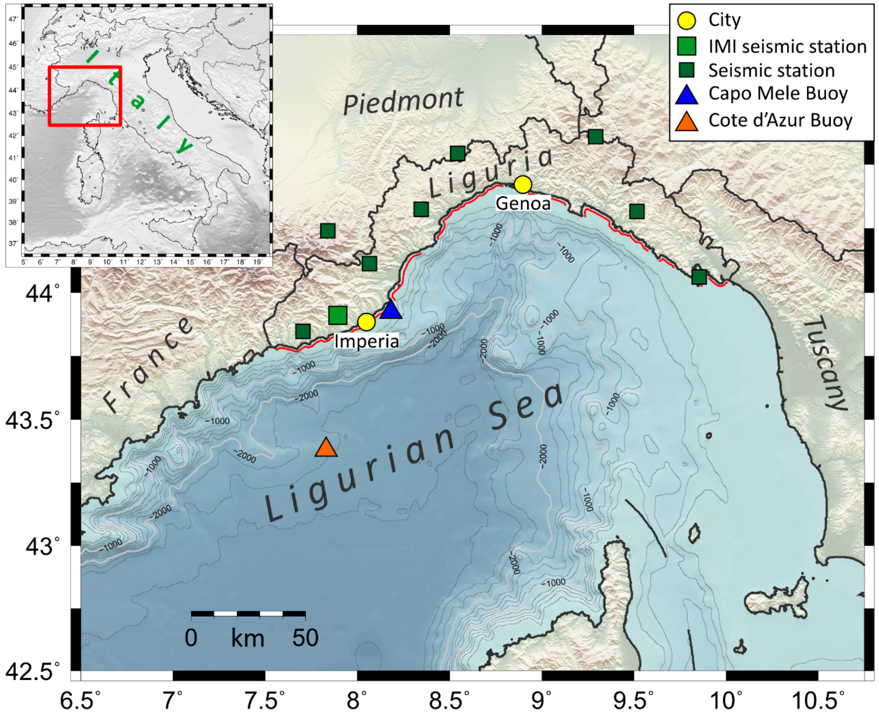
2. Study Area and General Features of the Adrian Storm

The study area (Figure 1) is the coastal part of the Ligurian Sea in the western Mediterranean Sea. The Ligurian Sea has a narrow continental shelf (with an average distance from the coast of 10 km) with steep slope incised by submarine canyons located along the main waterways of the region [30]. The Ligurian coast (about 330 km long) has steep arch-shaped mountains interspersed with wide valleys that control and channel the air movements. In the Ligurian Sea, the most frequent and significant sea storms are generated by winds from SE (Sirocco), SW (Libeccio), and NW (winds coming from the Gulf of Lion in cyclonic rotation; “short” Libeccio). These winds are usually related to perturbations from the Atlantic Ocean and Gulf of Lion, which carry strong, humid, and warm winds. These morphological and meteorological characteristics imply frequent events of heavy rainfall and rough sea and make the Ligurian Sea one of the most active areas of cyclogenesis in Europe [31,32,33,34,35], with strong and very rapid changes in weather conditions. In the past, the most destructive sea storms occurred in 1898 and 1955 (sea state > 7 of the Douglas Sea Scale), causing severe damage to the structures and vessels in the Port of Genoa [36].

On 27 October 2018, a deep trough between the Arctic Ocean and North African coasts was established on the Iberian Peninsula, and then moved eastwards and hit the whole Italian peninsula, causing an intense SW flow in the mid-troposphere and an SE flow in the lower layers. On 29 October, the cyclogenesis on the Gulf of Lion has deepened and the flow on the eastern edge of the cut-off was intense and from S, with a consequent recall of hot and humid air of African origin in the central Europe. In the Ligurian Sea, in the early hours of 29 October, a V-shape structure developed. It was characterised by a strong, self-regenerating convective activity with a high vertical development, which stationed on the basin for several hours. The convective activity was characterised by the continuous formation of new storm cells produced by the downdraft in the opposite direction to the main flow, which therefore caused the persistence of thunderstorm phenomena on the basin. This structure was generated by several factors: the strong flows from SW at high altitude due to the tiling on the western Mediterranean Sea, the presence of a high quantity of water vapour, a high convective available potential energy, and high values of equivalent potential temperature.

In the afternoon of 29 October, the entire Italian territory was affected by the passage of a cold front coming from W, along which a squall line (a very intense thunderstorm line) developed, accompanied by intense precipitation and numerous lightning strikes along the cold front line. This complex scenario brought very low-pressure values (≈978 hPa; Figure 2) which, combined with strong S winds, caused a storm surge phenomenon (i.e., a strong and rapid rise of the sea surface elevation) that contributed to increase the effect of the sea storm. At its maximum intensity, the storm was characterised by wind gusts over 150 km h⁻¹, H_s greater than 6 m, maximum wave height of 10 m, and peak wave period (T_p) of 11 s. This value of T_p is very rare in a closed sea such as the Mediterranean Sea. The development of the sea wave can be divided into two phases: a first phase during which the wave direction spanned between 120° and 160° (from 04:00 to 21:00 of 29 October), followed by a second phase during which the wave direction was mainly around 200°. In the Ligurian Sea, this shift in wave direction is very common during storm. In fact, the interaction of the synoptic flows with the complex mountain topography causes the development of deep orographic lows, usually very dynamic, that, in turn, cause very rapid transition of winds from SE to SW, with intensity strongly enhanced by coastal effects [37].

Since the night of 29 October, the perturbed system moved NE, leaving space for a gradual ascent of the geopotential field on 30 October [27,38,39].

3. Materials and Methods

3.1. Weather and Sea Data

In order to examine the distinctive peculiarities of the Adrian storm to improve the procedure proposed by Ferretti et al. [15] for monitoring H_s from microseism recordings during strong marine events, four significant sea storms that occurred in the Ligurian Sea in 2008 and between 2012 and 2018 were analysed and compared to the recent Adrian storm. Specifically, the considered the events occurred on 30 October 2008 (the sea storm already considered by Ferretti et al. [13]), 28 October 2012, 10 November 2013, and 25 December 2013 (three sea storms occurred in the period 2012–2018, for which continuous seismic recordings were available for analysis). All the sea storms considered were generated by strong southerly winds and showed H_s > 3 m. Data of sea wave characteristics, sea level, and atmospheric conditions were collected in order to highlight differences among these sea storms in terms of sea wave parameters and in terms of microseism characteristics.

For each selected sea storm, hourly H_s (in m), maximum individual sea wave height (H_max), wave direction and T_p were collected from buoys installed in the Ligurian Sea. In particular, for the event that occurred in 2008, we analysed data measured by the Côte d’Azur buoy (latitude 43.38° N, longitude 7.83° E, depth of anchoring 2300 m), which belongs to the Meteo-France network (www.shom.fr (accessed on 19 November 2020)). Concerning the 2012, 2013, and 2018 events, data measured by the buoy of Capo Mele (latitude—43.92° N, longitude—8.18° E, depth of anchoring—90 m), which is managed by the Ligurian Environmental Protection Agency (http://servizi-meteoliguria.arpal.gov.it/boacapomele.html (accessed on 19 November 2020)), were considered. Sea level (m), atmospheric pressure (hPa), and relative humidity (%) data measured during the five sea storms were collected from the tide gauge station of Imperia Porto Maurizio (part of the National Tide-gauge Network; www.mareografico.it (accessed on 19 November 2020)) located 13 km far off the Capo Mele buoy.

Wind direction (° N) and velocity (m s⁻¹) were obtained from the Seismic and Meteorological Observatory of Imperia (managed by the Municipality of Imperia; http://www.cartografiarl.regione.liguria.it/SiraQualMeteo/script/PubAccessoDatiMeteo.asp (accessed on 19 November 2020)) located 14 km SW off the Capo Mele buoy. The two measuring stations and the buoy of Capo Mele are not colocated, but given the relatively small distance between them, the effect of this distance on the results of the analyses is assumed negligible given the noninstantaneous inertia of the system (i.e., the sea).

All data were sampled hourly.

Starting from the water level records (provided by the station of Imperia Porto Maurizio), the storm surge series were computed for each of the investigated events. First, the tidal contribution was predicted through the Tidal Model Driver (TMD) package for MATLAB software (TMD software v. 2.05, [40]) provided by the Earth & Space Research (https://www.esr.org/research/polar-tide-models/tmd-software/ (accessed on 19 November 2020)). Then, the predicted tides were taken off the total water level, leading to the tidal residual. When tides are relevant, it is advisable to split the tidal residual in two contribution, i.e., a low-frequency and a high-frequency signal, corresponding to the meteorological-induced surge and the interaction between the tides and the surge [41]. However, given that in the Ligurian Sea the tidal oscillation accounts to a few centimetres at most over the total water level, we assumed the tidal residual was driven only by the storm surge.

In addition to the previous data, the distance between the Capo Mele buoy and the minimum of atmospheric pressure was estimated (in km) for each considered event. This distance can be useful to explain the oscillation of the microseism amplitude [25], and therefore to explain the relation between this latter and the H_s generated during the storms.

Finally, a statistical analysis was carried out in order to find the most influential atmospheric parameters during the Adrian storm. Specifically, the Redundancy Analysis (RDA) [42] multivariate technique was applied to explain the linear relationship between the explanatory variables, which are the atmospheric forcing (wind velocity, atmospheric pressure and pressure gradient), and the response variables, which are the sea responses to such forcing (storm surge, H_s, and T_p). For each storm and for each parameter of interest, the analyses were carried out on ordered time series of 25 hourly samples around the time of the H_max. Details of the method used for the RDA analysis are described in Cutroneo et al. [43]. The RDA was performed using the Brodgar software (Highland Statistics Ltd., v. 2.7.5, 2017).

3.2. Microseismic Data

In this study, we present the results of the analysis of the microseism recorded at the IMI station (Figure 1), which is the RSNI station closest to the Capo Mele buoy. For all storms, only the vertical component of the signals was considered.

Following Ferretti et al. [13,14,15], microseismic data were processed according to the following steps:

• Instrumental correction (deconvolution).
• Signal resampling at a frequency of 2 Hz.
• Offset and linear trend removal.
• Signal windowing into 1 hr windows.
• Computation of the Fourier transform for each window.
• Spectrogram calculation.

The spectral characteristics of the microseism were thus determined through Fourier amplitude spectra and spectrograms.

4. Results

Following the methods described above, the sea wave parameters (derived from measuring buoys and microseisms) and atmospheric pressure data were analysed for the five sea storms considered in this study.

4.1. Microseism Analysis

Figure 3 compares H_s measured by the buoys (red lines) and those obtained using microseism recordings according to the procedure of Ferretti et al. [15] (green lines). Except for the Adrian storm (Figure 3e) and for the initial phase of the November 2013 event (Figure 3c), H_s measured by the buoy and H_s estimated by microseism were similar with differences that, on average, are lower than 0.2 m. During the Adrian storm, the Capo Mele buoy measured H_s greater than 6 m, which are almost twice the values estimated using the microseism.

Figure 4 shows the characteristics of the microseism recorded at the IMI station during the five sea storms in terms of the Fourier amplitude spectra for different hourly signal windows and spectrograms. As already shown by Ferretti et al. [13], the microseism associated with sea storms in the Ligurian Sea is dominated by frequencies of around 0.2–0.3 Hz, whereas the microseism controlled by frequencies lower than 0.15 Hz is associated with storms located in the Atlantic Ocean. For all sea storms considered in the present study, the largest microseism amplitude concentrates around 0.2 Hz. During the 2008, 2012, and December 2013 events, the spectral amplitude at 0.2 Hz exceeded, on average, the value of 6 × 10⁻⁷ m s⁻¹, reaching values greater than 8 × 10⁻⁷ m s⁻¹. On November 2013, during the sea storm that generated the lowest H_max (

Table 1. Weather and sea data for the five sea storm events considered in this study. n.a.: not available.

Sea Storm	Sea storm Peak (dd/mm/yyyy hh:mm)	Period Considered for Weather Condition Evaluation (dd/mm/yyyy hh:mm)	Maximum Sea Wave Height (Hmax, m)	Maximum Significant Sea Wave Height (Hs, m)	Peak Sea Wave Period (Tp, s)	Mean Wave Direction during the Sea Storm Peak (° N)	Maximum Storm Surge (m)	Minimum Atmospheric Pressure (hPa)	Maximum of Mean Wind Velocity (m s−1)	Estimated Distance between the Capo Mele Buoy and the Minimum of Atmospheric Pressure (km) at the Maximum Hs Moment
October 2008	30/10/2008 n.a.	26/10/2008 00:00–31/10/2008 23:30	n.a.	3.7 1	n.a.	n.a.	n.a.	n.a.	n.a.	22
October 2012	28/10/2012 03:00	22/10/2012 00:00–28/10/2012 23:30	6.37	4.16	9.97	216	0.47	984.3	8.6	88
November 2013	10/11/2013 11:00	05/11/2013 11:00 2–10/11/2013 23:30	6.02	4.02	9.67	340	0.23	1000	9.7	25
December 2013	25/12/2013 23:00	20/12/2013 00:00–26/12/2013 23:30	8.40	5.14	10.5	185	0.29	984.4	11.3	105
October 2018	29/10/2018 22:00	24/10/2018 00:00–30/10/2018 23:30	9.61	6.08	11.7	246	0.61	977.7	16.1	25

¹ Significant sea wave height collected by the Côte d’Azur buoy [13]. ² Data before 05/11/2013 11:00 UTC were not available.

), the spectral amplitude of microseism slightly exceeded 4× 10⁻⁷ m s⁻¹ and a significant underestimation of the H_s provided by microseism (up to 1.5 m) was observed during the initial phase of the storm (Figure 3c). During the Adrian storm, the spectral amplitude of the microseism at 0.2 Hz remained nearly below 2 × 10⁻⁷ m s⁻¹.

It is noteworthy that the H_s values estimated using the procedure of Ferretti et al. [15] and reported in Figure 3 have been computed considering the microseism recordings provided by the RSNI seismic stations located along the Ligurian coast (the H_s values is calculated by averaging over the nine stations shown in Figure 1). The underestimation of the H_s provided by the procedure of Ferretti et al. [15] is due to the low energy of the microseism recorded along the Ligurian coast during the Adrian storm. In fact, all recordings provided by the other RSNI seismic stations located along the Ligurian coast (Figure 1) show microseism characteristics as similar as those observed at the IMI station. Moreover, the H_s values predicted by microseism show a significant underestimation at all target sites considered in Ferretti et al.’s [15] procedure and located along the Ligurian coast. The predicted H_s values never exceed 3.5 m at any target site while indirect observations (such as damages to coastal infrastructures) indicate sea waves with much greater heights along the entire Ligurian coast (see previous paragraphs).

Similar considerations on the microseism energy can be observed from the spectrograms (Figure 4). For the events occurred in 2008, 2012, and 2013, the spectral amplitude values for the frequencies dominating microseism recordings reached values greater than −65 dB, whereas during the Adrian storm they rarely exceeded −75 dB.

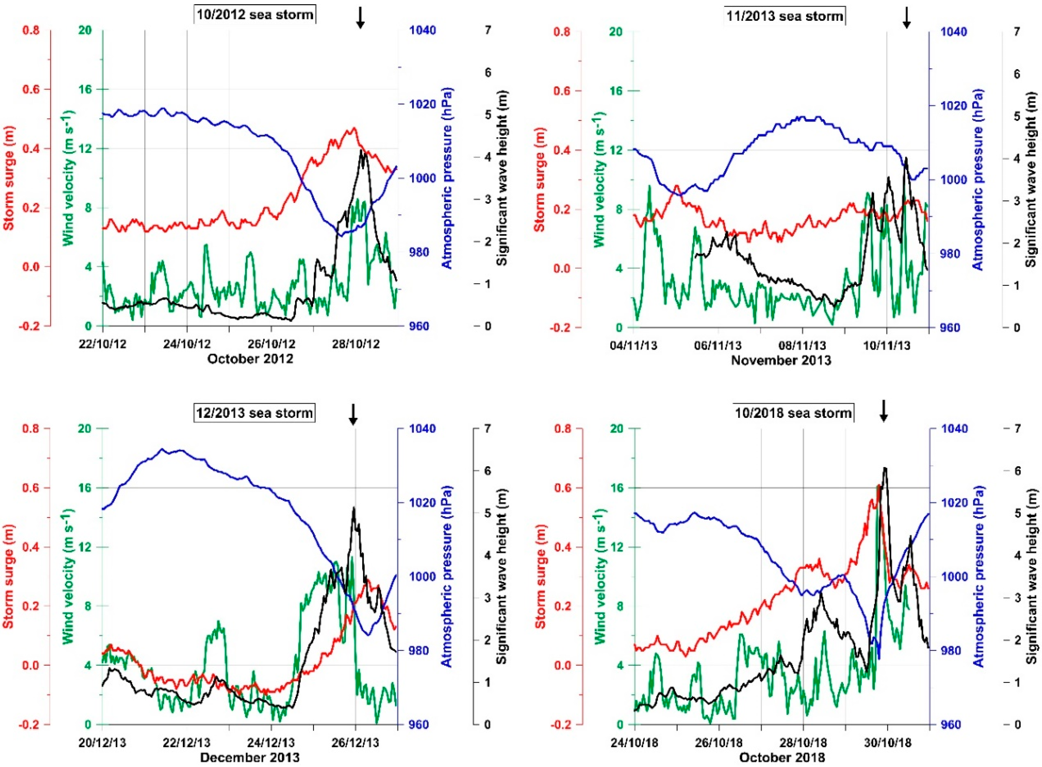
4.2. Weather and Sea Data Analysis

Table 1 summarises the main weather and sea parameters measured during the five sea storms considered. The H_max spans between 6 (November 2013 event) and 9.6 m (October 2018 event), whereas the maximum H_s spans between 3.7 (October 2008 event) and 6.1 m (October 2018 event). The T_p observed during the five sea storms ranges between 9.7 (November 2013 event) and 11.7 s (October 2018 event). The maximum storm surge is between 0.29 and 0.47 m for the 2012 and 2013 events and 0.61 m for the 2018 one. The minimum atmospheric pressure spans between 970 (October 2018 event) and 1,000 hPa (November 2013 event). The mean wind velocity reached a maximum of 11.3 m s⁻¹ for the 2012 and 2013 storms, while reached the maximum value of 16.1 m s⁻¹ during the 2018 storm. It appears clear that the Adrian storm has the highest H_s, the highest T_p, the highest storm surge, the lowest atmospheric pressure, and the highest mean wind velocity. The distance between the study area and the centre of the low pressure indicates two possible group of storms: the first group collects sea storms occurred when the pressure minimum was very close to the study area with distances of less than 25 km (October 2008, November 2013, and October 2018 events); the second group is characterised by distances greater than 88 km (October 2012 and December 2018 events).

Figure 5 shows the evolution of storm surge, atmospheric pressure, H_s, and mean wind velocity measured during four of the five sea storms considered (no data are available for the 2008 event). Noteworthy is the fact that the rapid decrease in the atmospheric pressure values, the strong increase in wind velocity, and the related large storm surge, were almost simultaneously only during the Adrian storm. In fact, during the 2012 storm, the minimum of atmospheric pressure preceded the increase in wind velocity and storm surge, while during the 2013 storms, the increase in wind velocity preceded the decrease in pressure and the rise of storm surge.

Figure 6 shows the time variation of H_s and the atmospheric pressure gradient for hourly time windows for the four sea storms. It is evident that the Adrian storm is associated with an anomalous baric gradient trend, showing a wider and steeper pressure variation occurred in a very short time.

Figure 7 summarises the results of RDA. In this plot, the angles between all vectors reflect their (linear) correlation. The correlation is equal to the cosine of the angle between vectors. Right-angled projections of observation points onto vectors representing response variables approximate variable values for a given observation. Considering the overall results of RDA, the atmospheric pressure is slightly more informative in terms of explaining the variability of the sea wave parameters, followed by the wind velocity. Considering individual parameters, the atmospheric pressure is positively related to T_p and negatively related to storm surge. Focusing on H_s, the most significant parameter in our study case (Figure 7) shows that H_s is strictly correlated with pressure gradient and wind velocity. Moreover, data recorded around the maximum development of the Adrian storm (data between 4_9 and 4_16 highlighted in light blue in Figure 7) are associated with the highest values of H_s, wind velocity and pressure gradient.

5. Discussion

Through the analyses performed in the present study, the distinctive peculiarities of the Adrian storm have been examined. With respect to the other storms considered, the Adrian storm showed very peculiar features in terms of microseismic energy and meteorological-oceanic parameters. Specifically, during the Adrian storm, the pressure gradient has been significantly steeper than during the other events, and the wind velocity and the storm surge resulted very high values. The microseismic frequency content was akin to the other storms, but its energy proved to be significantly lower, leading to an underestimation of the H_s value provided by the procedure proposed by Ferretti et al. [15].

The exceptionality of the Adrian storm was confirmed by comparison of its peculiar features with bibliographic data. For example, storm surge, primarily due to the wind associated with transit or stationery (24-48 h) low-pressure systems at medium latitudes [44], is generally weak in semienclosed basins such as the Mediterranean Sea. Ullmann and Pirazzoli [45], who analysed storm surges measured at three tide gauge stations located along the coast of the Gulf of Lions (north-western Mediterranean Sea) between 1948 and 2003, found that more than 80% of storm surges ≥ 0.60 m (as recorded during the Adrian storm) are associated with winds >10 m s⁻, which mostly contribute to the storm surge peak. Nevertheless, storm surge values ≥ 0.60 m are not frequent in the Mediterranean Sea, except for areas such as Venice lagoon (north-eastern Italy), and occur one time per season [45]. During the Adrian storm, the simultaneous strong decrease in atmospheric pressure and strong increase in wind speed, with a large fetch involving a vast portion of the Mediterranean, have contributed to the exceptional height of the storm surge. Moreover, during its peak, the sea waves were characterised by a peak period of 11.7 s, an extreme value relatively to the Mediterranean Sea. Pasi et al. [46] have observed that, in the period 1998–2010 (out of our study period), a sea storm characterised by a similar T_p occurred only once in the Ligurian Sea (on 1–2 January 2010) and, in the same 12-year period, they noted that sea storms with H_s greater than 4.3 m are generally characterised by mean wave periods of about 8.4 s.

Despite its meteorological-oceanic characteristics, the Adrian storm did not produce a high-energy microseism. As is well known, there is a strong correlation between H_s and local microseisms [13,14,15,47], but the generation mechanism of (primary) microseisms requires the sea surface-waves to interact with the sea bottom—namely, it occurs mainly in coastal areas with water shallower than half of the wavelength [48]. The correlation between sea waves and microseisms also depends on the duration of the storm; Traer et al. [48] found that sea waves typically evolve over a scale of days and that microseism features change with a similar time scale. Ardhuin et al. [49] found that an atmospheric perturbation that moves quickly and affects an area of shallow water near the coastline generates a weak conversion of wave-induced pressure to seismic noise. Therefore, sea waves produced by the Adrian storm had great energy, but their very rapid development, the position of the pressure minimum very close to the coast, and the very rapid variation of wave direction (from SE to SW) may have prevented the generation of a high-energy microseism. It is noteworthy that, a microseism with energy less than expected has also been observed during the November 2013 storm which developed very close to the Ligurian coast (see Table 1).

These effects along with a very high storm surge and a very high wind velocity may explain the nature of the Adrian storm, characterised by very high sea waves but a low-energy microseism. In summary, during this storm, the exceptional meteorological conditions (i.e., wind velocity and pressure gradient) and their spatial-temporal trend caused a peculiar response of the Ligurian Sea (in terms of storm surge, period and height of sea waves), linked to an anomalous microseism.

Although the mechanism of the microseism origin is difficult to discriminate in the Ligurian Sea, as already highlighted by Ferretti et al. [13], the secondary microseism, being by far stronger than the primary microseism, is probably the dominant influence on the microseism-based predictive models proposed by Ferretti et al. [15] for near real-time monitoring of H_s. Therefore, during the Adrian storm, because of the peculiarities listed above, the generation of a secondary microseism has been exceptionally low, leading to an underestimation of H_s. Unfortunately, at the moment, we cannot suggest any explanation for which the situation is not favorable for generating secondary microseisms during some storms (such the Adrian one). Following our results, in order to avoid a significant underestimation of the H_s during future extreme sea storm events and, therefore, to improve the effectiveness of the procedures for real-time monitoring of the H_s through microseismic data, we can only propose adding the pressure gradient together with the wind velocity into microseism-based predictive models. These parameters are nowadays easily available from weather station networks.

Therefore, an empirical correction of the prediction model is proposed here. According to our results, the correction term must be applied to the predictive model only when extreme values of wind velocity and pressure gradient are observed. Specifically, it is assumed the correction term must be applied only when the hourly wind velocity values or the absolute values of the pressure gradient exceed the 95^th percentile of data distribution. Considering data measured during the 2012, 2013, and 2018 events, the 95^th percentile of wind velocity and pressure gradient data distributions are 8.4 m s⁻¹ and 1.1 hPa h⁻¹, respectively.

The correction term has been derived and calibrated considering two main pieces of empirical evidence that are:

• the differences between H_s measured by the buoy and those obtained by microseism linearly increase when the wind velocity and the absolute values of pressure gradient increase;
• the increases in wind velocity and absolute values of pressure gradient produce an increase in H_s with a delay up to 5 h (Figure 8). Then, the most suitable correction parameters are estimated averaging six samples of wind velocity and absolute values of pressure gradient.

Finally, the model of Ferretti et al. [15] was modified accordingly as follows:

If

$$WM{V}_{i-6}>8.4 \left(m{s}^{-1}\right) or AP{G}_{i-6}>1.1 \left(hPa{h}^{-1}\right)i=1,\dots ,6$$

(1)

then

$$H_{s\_new}=H_{s\_est}+a*{\displaystyle \sum }_{i=1}^6\frac{WM{V}_{i-6}}{6}+b*{\displaystyle \sum }_{I=1}^6\frac{AP{G}_{i-6}}{6}$$

(2)

where WMV is the wind mean velocity, APG is the absolute value of pressure gradient, i indicates the sample number (e.g., i = 0 corresponds to the current time; i = −5 corresponds to the data measured five hours before), and H_{s_est} and H_{s_new} are the H_s estimated by the procedure of Ferretti et al. [15] before and after the correction, respectively.

Figure 9 compares the H_s measured by the buoy (blue line) and those provided by the procedure of Ferretti et al. [15] before (red line) and after (green line) the application of the proposed correction term for the Adrian storm. The differences between the H_s values measured by Capo Mele buoy and those obtained by using the microseism-based procedure corrected are strongly reduced (old maximum difference 3.4 m, new maximum difference 1.2 m). Since the applicability conditions were not met for the other sea storms (during which WMV and APG stayed under the thresholds), the correction term was not applied. It is worth highlighting that the thresholds, guiding the use of the correction term, were defined based on statistical analysis. Specifically, the thresholds of wind velocity and pressure gradient corresponds to the 95th percentile of data distributions. Among all storms that have occurred in Liguria since 2008, the Adrian storm is the only one that presents both wind velocity and pressure gradient values that exceed the thresholds chosen. However, it is worth noting that the data scarcity does not allow us to effectively verify the robustness of such a criterion for differentiating storms, and the wrong application of such a correction term to storms that generate high-energy microseisms could generate significant errors in the estimation of H_s.

6. Conclusions

In the present study, we compared the characteristics of five of the most significant sea storms that struck the Ligurian coast between 2008 and 2018. Specifically, we analysed both sea wave and atmospheric parameters and presented a spectral analysis of the storm-related microseisms. The aim was to highlight the distinctive features of the exceptional event occurred on October 2018 (Adrian storm) with respect to other strong sea storms in the same area in order to make (also during exceptional storms) the procedure proposed by Ferretti et al. [15] more effective for monitoring the sea wave height. In fact, although the Adrian storm caused sea wave heights of up to 9 m and significant damage to coastal infrastructures, it generated a very low energy microseism, thus leading to a severe underestimation of the H_s values assessed through the procedure proposed by Ferretti et al. [15]. Therefore, a correction term, that takes into account wind velocity and the atmospheric pressure gradient, was proposed and applied to the predictive model, allowing a significantly reduction in the underestimation of the estimated H_s when dealing with storms that generate low energy microseisms (such as the Adrian storm). In our case, the wind velocity and pressure data were provided by the weather station of the Seismic and Meteorological Observatory of Imperia and, therefore, the applicability of the proposed correction term is limited to the area around Imperia and Capo Mele buoy (Figure 1). For the Adrian storm, the inclusion of meteorological data (wind velocities and pressure gradients above an empirically determined threshold) together with the microseism amplitude in the prediction of significant wave height resulted in a significantly better fit. Whether this or a similar formula, although promising, is applicable in general must be validated by a larger dataset. It will also be necessary to monitor if the H_s estimation is realistic during other events similar to the Adrian storm, even in presence of different storm characteristics.

References

1. Devis-Morales, A.; Montoya-Sánchez, R.A.; Bernal, G.; Osorio, A.F. Assessment of extreme wind and waves in the Colombian Caribbean Sea for offshore applications. Appl. Ocean Res. 2017, 69, 10–26. [Google Scholar] [CrossRef]
2. Ardhuin, F.; Stopa, J.E.; Chapron, B.; Collard, F.; Husson, R.; Jensen, R.E.; Johannessen, J.; Mouche, A.; Passaro, M.; Quartly, G.D.; et al. Observing Sea States. Front. Mar. Sci. 2019, 6, 124. [Google Scholar] [CrossRef] [Green Version]
3. Mentaschi, L.; Besio, G.; Cassola, F.; Mazzino, A. Performance evaluation of Wavewatch III in the Mediterranean Sea. Ocean Model. 2015, 90, 82–94. [Google Scholar] [CrossRef]
4. O’Reilly, W.C.; Olfe, C.B.; Thomas, J.; Seymour, R.J.; Guza, R.T. The California coastal wave monitoring and prediction system. Coast. Eng. 2016, 116, 118–132. [Google Scholar] [CrossRef] [Green Version]
5. He, Y.; Shen, H.; Perrie, W. Remote Sensing of Ocean Waves by Polarimetric SAR. J. Atmos. Ocean. Tech. 2006, 23, 1768–1773. [Google Scholar] [CrossRef]
6. Yaakob, O.; Zainudin, N.; Samian, Y.; Maimun, A.; Malik, A.; Palaraman, R.A. Presentation and validation of remote sensing ocean wave data. IJRRAS 2010, 4, 373–379. [Google Scholar]
7. Reale, F.; Dentale, F.; Pugliese Carratelli, E.; Fenoglio-Marc, L. Influence of sea state on sea surface height oscillation from Doppler altimeter measurements in the North Sea. Remote Sens. 2018, 10, 1100. [Google Scholar] [CrossRef] [Green Version]
8. Ludeno, G.; Reale, F.; Raffa, F.; Centale, F.; Soldovieri, F.; Pugliese Carratelli, E.; Serafino, F. Integration between X-band radar and buoy sea state monitoring. Ocean Coast. Discuss. 2016, 1–16. [Google Scholar] [CrossRef] [Green Version]
9. Cui, J.; Bachmayer, R.; de Young, B.; Huang, W. Ocean wave measurement using short-range K-band narrow beam continuous wave radar. Remote Sens. 2018, 10, 1242. [Google Scholar] [CrossRef] [Green Version]
10. Bromirski, P.D.; Duennebier, F.K.; Stephen, R.A. Mid-ocean microseisms. Geochem. Geophy. Geosy. 2005, 6. [Google Scholar] [CrossRef]
11. Stutzmann, E.; Schimmel, M.; Patau, G.; Maggi, A. Global climate imprint on seismic noise. Geochem. Geophy. Geosy. 2009, 101. [Google Scholar] [CrossRef]
12. Ardhuin, F.; Gualtieri, L.; Stutzmann, E. How ocean waves rock the Earth: Two mechanisms explain microseisms with periods 3–300s. J. Geophys. Res. 2015, 42, 765–772. [Google Scholar] [CrossRef] [Green Version]
13. Ferretti, G.; Zunino, A.; Scafidi, D.; Barani, S.; Spallarossa, D. On microseisms recorded near the Ligurian coast (Italy) and their relationship with sea wave height. Geophys. J. Int. 2013, 194, 524–533. [Google Scholar] [CrossRef] [Green Version]
14. Ferretti, G.; Scafidi, D.; Cutroneo, L.; Gallino, S.; Capello, M. Applicability of an empirical law to predict significant sea-wave heights from microseisms along the Western Ligurian Coast (Italy). Continent. Shelf Res. 2016, 122, 36–42. [Google Scholar] [CrossRef]
15. Ferretti, G.; Barani, S.; Scafidi, D.; Capello, M.; Cutroneo, L.; Vagge, G.; Besio, G. Near real-time monitoring of significant sea wave height through microseism recordings: An application in the Ligurian Sea (Italy). Ocean Coast. Manag. 2018, 165, 185–194. [Google Scholar] [CrossRef]
16. Ardhuin, F.; Stutzmann, E.; Schimmel, M.; Mangeney, A. Ocean wave sources of seismic noise. J. Geophys. Res. 2011, 116, C09004. [Google Scholar] [CrossRef]
17. Davy, C.; Barruol, G.; Fontaine, F.R.; Sigloch, K.; Stutzmann, E. Tracking major storms from microseismic and hydroacoustic observations on the seafloor. Geophys. Res. Lett. 2014, 41, 8825–8831. [Google Scholar] [CrossRef] [Green Version]
18. Donne, S.; Nicolau, M.; Bean, C.; O’Neil, M. Wave Height Quantification Using Land Based Seismic Data with Grammatical Evolution. 2014. Available online: http://ncra.ucd.ie/papers/cec2014_waves.pdf (accessed on 11 March 2021).
19. University of Genoa. Regional Seismic Network of North-Western Italy; Other/Seismic Network; International Federation of Digital Seismograph Networks: Seattle, DC, USA, 1967. [Google Scholar] [CrossRef]
20. Mentaschi, L.; Besio, G.; Cassola, F.; Mazzino, A. Implementation and validation of a wave hindcast/forecast model for the west Mediterranean. J. Coast. Res. 2013, 65, 1551–1556. [Google Scholar] [CrossRef]
21. Chi, W.C.; Chen, W.J.; Kuo, B.Y.; Dolenc, D. Seismic monitoring of western Pacific typhoons. Mar. Geophys. Res. 2010, 31, 239–251. [Google Scholar] [CrossRef] [Green Version]
22. Chen, X.; Tian, D.; Wen, L. Microseismic sources during Hurricane Sandy. J. Geophys. Res. Solid Earth 2015, 120, 6386–6403. [Google Scholar] [CrossRef]
23. Davy, C.; Barruol, G.; Fontaine, F.R.; Cordier, E. Analyses of extreme swell events on La Réunion Island from microseismic noise. Geophys. J. Int. Oxf. Univ. Press (OUP) 2016, 207, 1767–1782. [Google Scholar] [CrossRef] [Green Version]
24. Lin, J.; Lin, J.; Xu, M. Microseisms generated by super typhoon Megi in the western Pacific Ocean. J. Geophys. Res. Oceans 2017, 122. [Google Scholar] [CrossRef] [Green Version]
25. Butler, R.; Aucan, J. Multisensor, microseismic observations of a hurricane transit near the ALOHA Cabled Observatory. J. Geophys. Res. Solid Earth 2018, 123, 3027–3046. [Google Scholar] [CrossRef]
26. Xiao, H.; Xue, M.; Yang, T.; Liu, C.; Hua, Q.; Xia, S.; Huang, H.; Manh Le, B.; Yu, Y.; Huo, D.; et al. The characteristics of microseisms in South China Sea: Results from a combined data set of OBSs, broadband land seismic stations, and a global wave height model. J. Geophys. Res. Solid Earth 2018, 123, 3923–3942. [Google Scholar] [CrossRef]
27. Pedemonte, L.; Corazza, M.; Forestieri, A.; Turato, B. Rapporto di Evento Meteorologico del 27-30/10/2018. Ligurian Environmental Protection Agency—Weather-Hydrological Functional Center of Civil Protection of the Liguria Region. 2019; p. 16. Available online: https://www.arpal.gov.it/contenuti_statici//pubblicazioni/rapporti_eventi/2018/REM_20181027-30_rossaBCDE_vers20190107.pdf (accessed on 11 March 2021).
28. Casella, E.; Rovere, A.; Pedroncini, A.; Mucerino, L.; Casella, M.; Cusati, L.A.; Vacchi, M.; Ferrari, M.; Firpo, M. Study of wave runup using numerical models and low-altitude aerial photogrammetry: A tool for coastal management. Estuar. Coast. Shelf Sci. 2014, 149, 160–167. [Google Scholar] [CrossRef]
29. Decreto del Commissario Delegato n. 2/2019. Eccezionali Eventi Meteorologici che Hanno Interessato il Territorio Della Regione Liguria nei Giorni 29 e 30 Ottobre 2018—OCDPC n.558/2018. Approvazione Elenco Comuni Danneggiati. Available online: https://www.regione.liguria.it/components/com_publiccompetitions/includes/download.php?id=32935:cdc-558-2-2019.pdf (accessed on 18 January 2021).
30. Corradi, N.; Zaquini, M.; Ferretti, O. Interpretazione Sismostratigrafica Della Piattaforma Costiera Antistante la Foce Dell’Entella. ENEA “Il Golfo del Tigullio—Liguria Orientale. Avanzamento Degli Studi per la Creazione di Strumenti Della Gestione Costiera”. 2003. Available online: http://www.santateresa.enea.it/wwwste/dincost/dincost_pdf/7sismica.pdf (accessed on 11 March 2021).
31. Capello, M.; Cutroneo, L.; Ferretti, G.; Gallino, S.; Canepa, G. Changes in the physical characteristics of the water column at the mouth of a torrent during an extreme rainfall event. J. Hydrol. 2016, 541, 146–157. [Google Scholar] [CrossRef]
32. De Leo, F.; Solari, S.; Besio, G. Extreme waves analysis based on atmospheric patterns classification: An application along the Italian coast. Nat. Hazards Earth Syst. Sci. Discuss. 2020, 20, 1233–1246. [Google Scholar] [CrossRef]
33. Lionello, P.; Abrantes, F.; Congedi, L.; Dulac, F.; Gacic, M.; Gomis, D.; Goodess, C.; Hoff, H.; Kutiel, H.; Luterbacher, J.; et al. Introduction: Mediterranean climate—Background information. In The Climate of the Mediterranean Region; Lionello, P., Ed.; Elsevier: Oxford, UK, 2012. [Google Scholar]
34. Pensieri, S.; Bozzano, R.; Schiano, M.E. Comparison between QuikSCAT and buoy wind data in the Ligurian Sea. J. Marine Syst. 2010, 81, 286–296. [Google Scholar] [CrossRef]
35. Sartini, L.; Cassola, F.; Besio, G. Extreme waves seasonality analysis: An application in the Mediterranean Sea. J. Geophys. Res. Oceans 2015, 120, 6266–6288. [Google Scholar] [CrossRef] [Green Version]
36. Gallino, S.; Benedetti, A.; Onorato, L. Wave watching. In Lo Spettacolo Delle Mareggiate in Liguria; Hoepli: Milano, Italy, 2016; p. 182. [Google Scholar]
37. Orlandi, A.; Pasi, F.; Onorato, L.f.; Gallino, S. An observation and numerical case study of a flash sea storm over the Gulf of Genoa. Adv. Sci. Res. 2008, 2, 107–112. [Google Scholar] [CrossRef]
38. Cavaleri, L.; Bajo, M.; Barbariol, F.; Bastianini, M.; Benetazzo, A.; Chiggiato, J.; Davolio, S.; Ferrarin, C.; Magnusson, L.; Papa, A.; et al. The October 29, 2018 storm in Northern Italy—An exceptional event and its modeling. Prog. Oceanogr. 2019, 178, 102–178. [Google Scholar] [CrossRef]
39. Celano, M.; Costa, S.; Foraci, R. Rapporto dell’evento meteorologico dal 27 al 30 ottobre 2018. Servizio Idro-Meteo-Clima. 2018, p. 49. Available online: https://allertameteo.regione.emilia-romagna.it/documents/20181/437770/Evento+27-30+ottobre+2018/ab59ec27-27c2-4793-b6f9-b0a91ceef30e (accessed on 11 March 2021).
40. Erofeeva, S.; Padman, L.; Howard, S.L. Tide Model Driver (TMD) Version 2.5, Toolbox for Matlab, GitHub. Available online: https://www.github.com/EarthAndSpaceResearch/TMD_Matlab_Toolbox_v2.5 (accessed on 18 January 2020).
41. Feng, X.; Olabarrieta, M.; Valle-Levinson, A. Storm-induced semidiurnal perturbations to surges on the US Eastern Seaboard. Cont. Shelf Res. 2016, 114, 54–71. [Google Scholar] [CrossRef] [Green Version]
42. Zuur, A.F.; Ieno, E.N.; Smith, G.M. Analysing Ecological Data; Springer: New York, NY, USA, 2007. [Google Scholar]
43. Cutroneo, L.; Castellano, M.; Carbone, C.; Consani, S.; Gaino, F.; Tucci, S.; Magrì, S.; Povero, P.; Bertolotto, R.M.; Canepa, G.; et al. Evaluation of the boundary condition influence on PAH concentrations in the water column during the sediment dredging of a port. Mar. Pollut. Bull. 2015, 101, 583–593. [Google Scholar] [CrossRef]
44. Vousdoukas, M.I.; Voukouvalas, E.; Annunziato, A.; Giardino, A.; Feyen, L. Projections of extreme storm surge levels along Europe. Clim. Dyn. 2016, 47, 3171–3190. [Google Scholar] [CrossRef] [Green Version]
45. Ullmann, A.; Pirazzoli, P.A. Recent evolution of extreme sea surge-related meteorological conditions and assessment of coastal flooding risk on the gulf of Lions. Méditerranée 2007, 108, 69–76. [Google Scholar] [CrossRef] [Green Version]
46. Pasi, F.; Orlandi, A.; Onorato, L.F.; Gallino, S. A study of the 1 and 2 January 2010 sea-storm in the Ligurian Sea. Adv. Sci. Res. 2011, 6, 109–115. Available online: www.adv-sci-res.net/6/109/2011/ (accessed on 1 February 2021). [CrossRef]
47. Bromirski, P.D.; Flick, R.E.; Graham, N. Ocean wave height determined from inland seismometer data: Implications for investigating wave climate changes in the NE Pacific. J. Geophys. Res. 1999, 104, 20753–20766. [Google Scholar] [CrossRef]
48. Traer, J.; Gerstoft, P.; Bromirski, P.D.; Shearer, P.M. Microseisms and hum from ocean surface gravity waves. J. Geophis. Res. 2012, 117, B11307. [Google Scholar] [CrossRef] [Green Version]
49. Ardhuin, F.; Balanche, A.; Stutzmann, E.; Obrebski, M. From seismic noise to ocean wave parameters: General methods and validation. J. Geophys. Res. 2012, 117, C05002. [Google Scholar] [CrossRef] [Green Version]
Figure 1. Location of the Imperia seismic station (IMI; large green square), the other Regional Seismic network of north-western Italy (RSNI) seismic stations located near the Ligurian coast (small green squares) and the two buoys (Capo Mele—Italy and Cote d’Azur—France; blue and orange triangles, respectively) considered in this study. The tide gauge station of Imperia Porto Maurizio and the weather station of the Seismic and Meteorological Observatory of Imperia are located in the city of Imperia. Red line shows the coastal area affected by damages.
Jmse 09 00319 g001
Figure 2. Maps of the mean sea level pressure (hPa, grey lines and colour fill) and geopotential height (m, black lines) on 29 October 2018 during the Adrian storm [27].
Jmse 09 00319 g002
Figure 3. Comparison between the significant sea wave heights (Hs) measured by the buoys (red lines) and those estimated using microseism recordings (green dotted lines) during the five considered sea storm events: (a) October 2008; (b) October 2012; (c) November 2013; (d) December 2013; (e) October 2018. The time window considered is not the same for all sea storms due to lack of data.
Jmse 09 00319 g003
Figure 4. Fourier amplitude spectra (normalised to the duration of the signal) for all one-hour windows in which each microseism recording was divided (on the left) and spectrogram of the vertical component of the microseism recorded during the five sea storms under study (on the right). (a) October 2008; (b) October 2012; (c) November 2013; (d) December 2013; (e) October 2018. The time window considered is not the same for all sea storm due to lack of data.
Jmse 09 00319 g004
Figure 5. Storm surge (red lines), atmospheric pressure (blue lines), mean wind velocity (green lines) measured by the Imperia stations, and significant sea wave height (black lines) measured by the Capo Mele buoy. Black arrows indicate the time of the maximum sea wave height.
Jmse 09 00319 g005
Figure 6. Significant wave height (m, black lines) superimposed on the temporal variation of the baric gradient (hPa, red lines) for hourly time window for a period of seven days around the sea storms of October 2012, November and December 2013, and October 2018.
Jmse 09 00319 g006
Figure 7. Redundancy Analysis (RDA) plot showing the relationship between the explanatory variables (Wind_vel: wind velocity; Atm_press: atmospheric pressure; Press_grad: gradient of atmospheric pressure) and response variables (Storm_surge: storm surge; Hs: significant sea wave height; Tp: peak period of sea wave). Each event is indicated using double numbering: the first number indicates the sea storm event (1: October 2012; 2: November 2013; 3: December 2013; 4: October 2018) while the second one indicates the sample number (from 1 to 25). The sum of all canonical eigenvalues is 0.34.
Jmse 09 00319 g007
Figure 8. Hs measured (blue line), pressure gradient (violet line) and wind velocity (orange line) during the Adrian storm.
Jmse 09 00319 g008
Figure 9. Comparison between Hs measured by the buoy (blue line) and those provided by model of Ferretti et al. [15] before (red line) and after (green line) the application of the correction term.
Jmse 09 00319 g009