Article

Synergy between Satellite Altimetry and Optical Water Quality Data towards Improved Estimation of Lakes Ecological Status

1
Tartu Observatory, University of Tartu, Observatooriumi 1, Tõravere, 61602 Tartu, Estonia
2
Division of Geodesy and Earth Observation, DTU Space, National Space Institute, 2800 Kgs. Lyngby, Denmark
3
Chair of Hydrobiology and Fishery, Institute of Agricultural and Environmental Sciences, Estonian University of Life Sciences, Kreutzwaldi 5, 51006 Tartu, Estonia
*
Author to whom correspondence should be addressed.
Remote Sens. 2021, 13(4), 770; https://doi.org/10.3390/rs13040770
Submission received: 30 December 2020 / Revised: 3 February 2021 / Accepted: 17 February 2021 / Published: 19 February 2021
(This article belongs to the Special Issue Remote Sensing of the Aquatic Environments)

Abstract

:
European countries are obligated to monitor and estimate ecological status of lakes under European Union Water Framework Directive (2000/60/EC) for sustainable lakes’ ecosystems in the future. In large and shallow lakes, physical, chemical, and biological water quality parameters are influenced by the high natural variability of water level, exceeding anthropogenic variability, and causing large uncertainty to the assessment of ecological status. Correction of metric values used for the assessment of ecological status for the effect of natural water level fluctuation reduces the signal-to-noise ratio in data and decreases the uncertainty of the status estimate. Here we have explored the potential to create synergy between optical and altimetry data for more accurate estimation of ecological status class of lakes. We have combined data from Sentinel-3 Synthetic Aperture Radar Altimeter and Cryosat-2 SAR Interferometric Radar Altimeter to derive water level estimations in order to apply corrections for chlorophyll a, phytoplankton biomass, and Secchi disc depth estimations from Sentinel-3 Ocean and Land Color Instrument data. Long-term in situ data was used to develop the methodology for the correction of water quality data for the effects of water level applicable on the satellite data. The study shows suitability and potential to combine optical and altimetry data to support in situ measurements and thereby support lake monitoring and management. Combination of two different types of satellite data from the continuous Copernicus program will advance the monitoring of lakes and improves the estimation of ecological status under European Union Water Framework Directive.

Graphical Abstract

1. Introduction

Consistent monitoring and estimation of the ecological status of lakes is essential for having an overview of current conditions and prediction of water quality (WQ) [1,2]. As lakes regulate the climate and carbon cycle, provide habitat for biota, drinking water, and other ecosystem services, it is important to monitor their ecological status and indications of their decline. To implement water management for sustainable environment, it is essential to evaluate the influence of human activity to lake ecosystems and also take into account variability of natural factors [3,4]. The European Union (EU) has established Water Framework Directive (2000/60/EC) [5] (WFD) for all European countries to achieve at least “good” ecological status class in lakes through consistent monitoring and water policy by the latest 2027 [6,7]. In total, five ecological quality classes from “high” to “bad” have been determined for every defined natural water body type, according to different biological (e.g., phytoplankton), physico-chemical (e.g., transparency) and hydro-morphological (e.g., depth variations) quality elements [5]. The main emphasis is given to the biological quality elements while the physico-chemical and hydro-morphological quality elements only affect the decision indirectly through their effect on the state of biological elements [5].
Traditional in situ measurements (e.g., collection of water samples, laboratory analyses, gauging stations, etc.) tend to be money and time consuming, and tend to take a lot of resources [8]. It is difficult to collect data from remote areas, where infrastructure is missing and access to the water body is complicated [9]. In situ gauging stations provide more frequent data than traditional measurements, but transmission of the data to the further workflow is rather slow and time consuming [10,11,12]. These kinds of systems are usually expensive to buy and difficult to maintain, therefore the number of gauging stations has decreased in recent years [11,12,13,14]. As lakes are mostly categorized as heterogeneous bodies, the biggest disadvantage of traditional in situ measurements is providing only point measurements, which do not represent spatial and temporal variations of the entire water body [1,11,15]. The combination of Earth Observation (EO) and in situ measurements complement each other by fulfilling their shortages and also helps to optimize and improve the selection of sampling locations and surveying times [16,17,18]. Earth Observation gives opportunity to have large scale data for spatial analysis and synchronized view of group of lakes [8,19]. In addition, digital data forms accelerates data reading and processing time and helps to produce historical and long time series [15]. The European Space Agency’s (ESA) Copernicus program [20] provides full, free, open access, high quality near-real-time EO data on a global level for all users. Since the launch of the first Sentinel mission satellite in 2014, the purpose of the program is to launch nearly 20 satellites by the year of 2030 to provide long-term time series for various applications, e.g., environmental protection, climate change monitoring, and civil security [21]. The continuity of data allows to develop and advance methods to better integrate EO data into environmental monitoring, management, and policy.
As the satellite era has lasted almost 40 years by now, many algorithms and methods have been developed for different domains in lake research [10,22,23,24,25,26,27,28,29,30,31]. As the WFD requirements are obligatory to every EU country, it has been indicated that the in situ methods are not feasible to cover the monitoring expectations, therefore many EO-based applications have been developed for implementation of requirements of WFD [32]. According to the WFD, phytoplankton is the key parameter of estimating ecological status of water [33,34,35,36], which also indicates eutrophication status of the lake [37]. Estimation of the concentration of the photosynthetic pigment chlorophyll a (chl a) has been one of the main goals in all ocean color missions starting from the first National Aeronautics and Space Administration (NASA) Coastal Zone Color Scanner on board Nimbus-7 in 1978. Additionally, water transparency is one of the key indicators for lake’s ecological status class according to the WFD [38,39,40], where also EO-based assessment methods have shown the suitability to obtain additional information [7,25,32,41]. Covering various ocean color missions, the approaches and algorithms have been developed to provide trophic status based estimations [31,42,43,44,45,46,47,48] to obtain chl a and transparency estimates. However, estimation is based only on certain parameters (e.g., chl a and transparency), which do not take into account any external factors [34,35,38,49]. Ranges of different ecological status classes of lakes may be very narrow, which is the main reason why accurate WQ parameter estimation is essential. Water level (WL) estimation, using satellite altimetry data over inland water bodies, has become more advanced during recent years [10,16,17,50,51,52], which allows the monitoring of its influence on the physical environment, which in turn changes the biota and whole lake ecosystem [53], especially in the case of shallow lakes.
In general, the ecological status of lakes is affected by anthropogenic factors, such as agricultural pollution by nutrients and industrial waste and various chemical elements [54], nevertheless natural factors, such as diurnal and seasonal changes, and prolonged changes in atmospheric circulations should be taken into account as well [55,56,57]. Water level is one of the natural factors, which affects WQ directly, worsening WQ parameters in low WL periods [58,59]. Especially in large, shallow lakes, the influence of lake depth variations on biota is remarkable, due to large seasonal and inter-annual WL fluctuations. The periods of extremely low WL are the most critical for the ecological status in such lakes, strengthening sediment resuspension, increasing concentrations of ions, phytoplankton biovolume and chl a concentration [60]. In contrast, the phytoplankton biomass (FBM) is significantly lower due to light limitation in years of high WL [61]. Such high variation in biological quality indicators, caused by natural factors, may over-mask human induced effects on a water body [62]. Based on the long-term in situ data, Tuvikene et. al. [62] showed the significant influence of WL while estimating the ecological status class according to the chl a, FBM and transparency in case of large shallow lakes. It was shown that, while phytoplankton species composition and traditional WQ parameters indicated different ecological status class, correction of metrics for WL enabled more consistent assessment of the ecological status of the lake.
As assessment of ecological status of lakes is currently parameter-based, thus accounting for the external natural factors is needed for more precise estimation. In the increasing constellation of ocean color satellites, carrying passive optical sensor usable for mapping various optical WQ parameters, and altimeters for estimating WL, the synergy of data could potentially improve the ecological status assessment over large shallow lakes. Therefore, the aim of this paper is to (1) create synergy between the optical and altimetry data in order to, (2) derive chl a, total FBM and transparency based ecological status classes taking into account the dependence of biological status indicators on the changing WL over large shallow lakes.

2. Materials and Methods

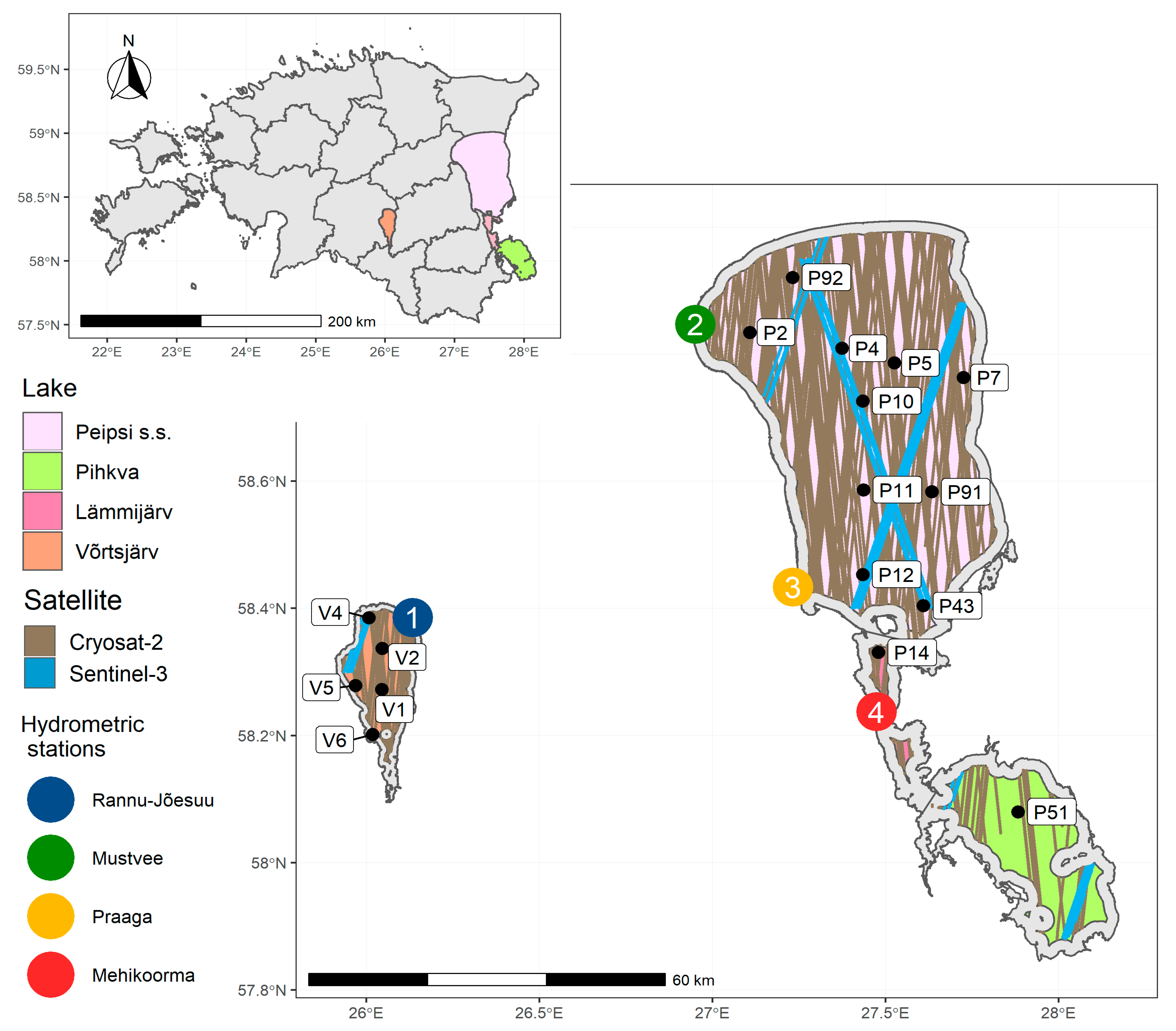
2.1. Study Sites Description

Data from two large and shallow lakes are used for this study. Võrtsjärv is situated in the central part of Estonia (Figure 1) with surface area 270 km2 (length 35 km, width ~14 km). With the average depth of 2.8 m (the maximum depth is 6 m), the lake has strong WL fluctuation as the annual mean amplitude is 1.4 m and absolute range is 3.1 m, causing up to 3.2-fold difference in the lake volume [61]. Water level is generally characterized by a high period in spring, due to snow melting until end of April or beginning of May, a low period in winter and summer, and increasing WL from middle of the October due to autumn rainfalls. Võrtsjärv is a eutrophic lake with low water transparency (<1 m) [63]. According to the Estonian regulation of Water Act [64], Võrtsjärv belongs to independent ecological status class Type 6 (Table 1) (non-stratified, light water color, low amount of chlorides, moderate hardness, surface area 100–300 km2). Annually, national monitoring is performed at one station once in a month and from additional 2 or 9 stations in August [65].
Peipsi is a transboundary lake situated in the border of Estonia and Russia (Figure 1) with surface area 3555 km2 (length 152 km, width 48 km). The average depth is 7.1 m (the maximum depth is 15.3 m) and the annual mean amplitude of WL change is 1.5 m. Water level of Peipsi is characterized the highest in spring during the ice melting period and is the lowest in October [66]. It is a eutrophic lake, which consists of three parts: Peipsi sensu stricto (s.s., 2611 km2 average depth 8.3 m), Lämmijärv (236 km2 average depth 2.5 m) and Pihkva (708 km2, average depth 3.8 m). According to the Estonian regulation of Water Act [8], Peipsi belongs also to the independent ecological status class Type 7 (Table 1) (non-stratified, light water color, low amount of chloride, moderate hardness, surface area >1000 km2) and is monitored 7 times per year (in March, when the lake is ice-covered, and from May to October) from 7 stations [65].
The both lakes are eutrophic and shallow, with similar WL fluctuation in terms of the annual mean (Võrtsjärv 1.4 m and Peipsi 1.5 m), but with different average depth (Võrtsjärv 2.8 m and Peipsi 7.1 m) leading to differences in the effect of WL. In addition, both lakes were considered unique, having no undisturbed reference sites for comparison, therefore, pressure-based approach, morphoedaphic index, and historical data were used to derive site-specific reference conditions and classification criteria for them [67].

2.2. In Situ Data

2.2.1. Water Level

Water level was measured by the Vaisala automatic weather station named as MAWS110, which sensor was located near the bottom of the lake and it measured the pressure of the water column, which is converted to the WL in centimeters [68]. Measurements were performed every hour, but WL was averaged over a day for the study. To derive WL above sea level (in Estonian Height system (EH2000), which corresponds to European Vertical Reference System), height of the sensor from sea level (national geoid named as EST-GEOID2017 (Estonian national geoid model)) [69] was added. Hydrometric stations were located near the shore or in the mouth of the river (Figure 1). Water level data was available in Rannu–Jõesuu (hereafter Rannu) hydrometric station from 1927, in Mustvee and Praaga from 1921 and in Mehikoorma from 1949 until 2019.

2.2.2. Chl a, FBM, and SDD

Chl a and FBM samples of integral water at discrete depths (0.5 m, 1 m, etc., until 0.5 m from the bottom) were collected from different stations and analyzed in a laboratory from the 1960s. Chl a samples were filtered through Whatman glass-microfiber filters (GF/F) ø 25 mm filter and pigment extraction was done with 5 mL 96% ethanol [70]. Chl a was measured spectrophotometrically with Hitachi U-3010 (430–750 nm) and the concentrations of chl a were derived according to Jeffrey and Humphrey [71]. For determination of FBM, up to 400 counting units were counted and measured with an inverted microscope based on Utermöhl technique [72]. SDD values were measured with white Secchi disc from the 1950s.

2.3. Satellite Data

Sentinel-3A/3B (S3A/S3B) and CryoSat-2 (C2) data from 2016 to 2019 covering the period from May to October were used. Buffers of 1 km (Võrtsjärv) and 2 km (Peipsi) were created to reduce the possible errors in the vicinity of land in case of optical and altimetry data (Figure 1). Depending on the cloud cover, 300 m resolution data from S3 Ocean and Land Colour Instrument (OLCI) is available daily in the study location. Surface elevations from the Synthetic Aperture Radar Altimeter (SRAL) sensor onboard S3A and S3B are available every 27 days for a given track. Lake Peipsi is measured by both S3A and S3B, hence, data are available from 2016 and onwards. Lake Võrtsjärv is only measured by S3B, hence data are available from the launch in 2018. C2, carrying Synthetic Aperture Radar/Interferometric Radar Altimeter (SIRAL) sensor, is operating in a geodetic orbit with a repeat period of 369 days. S3 and C2 tracks during the study period are shown on the Figure 1 in blue and gray, respectively.

2.3.1. Optical Data

S3 OLCI Level-1 (L1B) Full Resolution “Non Time Critical” images were used from Estonian National Satellite images database named as ESTHub [73]. Data were used from the beginning of S3 operation, respectively, S3A since 2016, and additional data from S3B since 2018. L1B data was filtered by quality flags (“bright”, “sun_glint_risk”, “duplicated”, “invalid”) and phytoplankton related parameters were derived via lake specific empirical relationship (Equations (2) and (3)) [74] applied on Maximum Chlorophyll Index (MCI) (Equation (1)) [75]:
M C I = L 709 L 681 709 681 753 681 × ( L 753 L 681 )
where Lx corresponds to top-of-atmosphere radiance at certain wavelength.
C h l   a = 10.9 × M C I + 15.3
F B M = 5.8 × M C I + 5.4
For water transparency estimates, OLCI L1B data was processed with Polymer v4.10 for retrieving water-leaving reflectance (ρw). Processed data were filtered by quality flag Bitmask (“0”, “1024”, “1023”). For the SDD estimates, first the weighting function (Equation (4)) [39] was applied on ρw which defined the appropriate empirical algorithm to derive diffuse attenuation coefficient of downwelling irradiance (Kd(490)) (Equation (5)).
W = 5.098 2.2099 ( ρ ( 560 ) ρ ( 709 ) )
K d ( 490 ) = ( 1 W ) × exp ( 0.9 ( log 10 ( ρ 490 ρ 709 ) + 0.4 ) + 0.02 ) + W × exp ( 1.2 ( log 10 ( ρ 560 ρ 709 ) + 1.4 ) + 0.02 )
Calculated W 0 corresponds to more transparent waters and algorithm ( ρ 490 / ρ 709 ) was used by assigning W = 0 . Calculated W 1 corresponds to more turbid waters and the algorithm ρ 560 / ρ 709 was used by assigning W = 1 . When the W is between 0 and 1, then the algorithm merges the retrievals from both ( ρ 490 / ρ 709   and   ρ 490 / ρ 709 ) algorithms [39].
Secondly, the SDD was derived based on the empirical algorithm from Kd(490):
S D D V õ r t s j ä r v = 0.038 × K d ( 490 ) + 0.9448
SDD for Peipsi s.s. (Equation (7)) was calculated using band ratio Kd(490) algorithm (Equation (5)) [38]:
S D D P e i p s i   s . s . = 3.42 × K d ( 490 ) 0.82
SDD for Lämmijärv and Pihkva was calculated using empirical algorithm (Equation (8)) [38]:
S D D L ä m m i j ä r v , P i h k v a = ( ρ ( 490 ) ρ ( 709 ) ) 0.7 × 2.14

2.3.2. Altimetry Data

To construct water surface elevations from S3A and S3B the ESA “Non Time Critical” Level-2 product “Enhanced measurements” was used. This product consists of 20Hz along-track measurements of, e.g., tracker range, satellite altitude, atmospheric and geophysical corrections, and waveforms. To identify the nadir water surface, the waveforms were retracked with a narrow primary peak threshold retracker [76]. For C2 we applied the ESA L1B product from baseline D. This product also contains 20Hz measurements of, e.g., waveforms, tracker range, satellite altitude and corrections. The same retracker was applied to the C2 waveforms.
The water surface elevations are derived from the following relation (Equation (9))
H = h R N ,
where h is the altitude of the satellite, and N is the geoid height, which here is the EST-GEOID2017 national geoid model. R is the range, i.e., the distance from the satellite to the surface which can be expressed as (Equation (10))
R = R t r a c k e r + R r e t r a c k + R a t m + R g e o .
Here R t r a c k e r is the distance to the presumed surface measured by the onboard tracker and R r e t r a c k is the retracking correction. R a t m represents the atmospheric corrections consisting of the wet and dry troposphere and ionosphere. R g e o represents the geophysical corrections including solid earth tide, pole tide, and ocean loading tide. All corrections are here taken from the altimetry products.
The altimetry-based WL time series based for Peipsi and Võrtsjärv were reconstructed using the “R” package “tsHydro” available from https://github.com/cavios/tshydro (accessed on 14 October 2020). The software package is based on an implementation of a simple state-space model where the observations are assumed to be described by a random walk plus noise. The observation noise is described by a mixture of a Normal and the heavy tailed Cauchy distributions making it more robust against erroneous observation. In the solution, bias between the different missions is also estimated. The model is described in detail in [10]. Here, one time series based on all available altimetry data is constructed for each lake.

2.4. Data Correction for the Effects of Water Level

EO-derived WQ variables (chl a, FBM, SDD) were corrected for the effects of changing WL by the methodology developed by Tuvikene et al. [62]. The methodology is based on the long-term in situ data, where statistically significant relationships (p-value < 0.05) between the specific WQ variables and WL were found (Table A1). Corrected WQ variables were calculated using regression equations according to the long-term monthly mean WL and daily measured WL. If the WL of the sampling day corresponded to the long-term average for that period, no correction was needed, but if it differed, the correction either up or down was proportional to the deviation of the WL from the mean.

3. Results

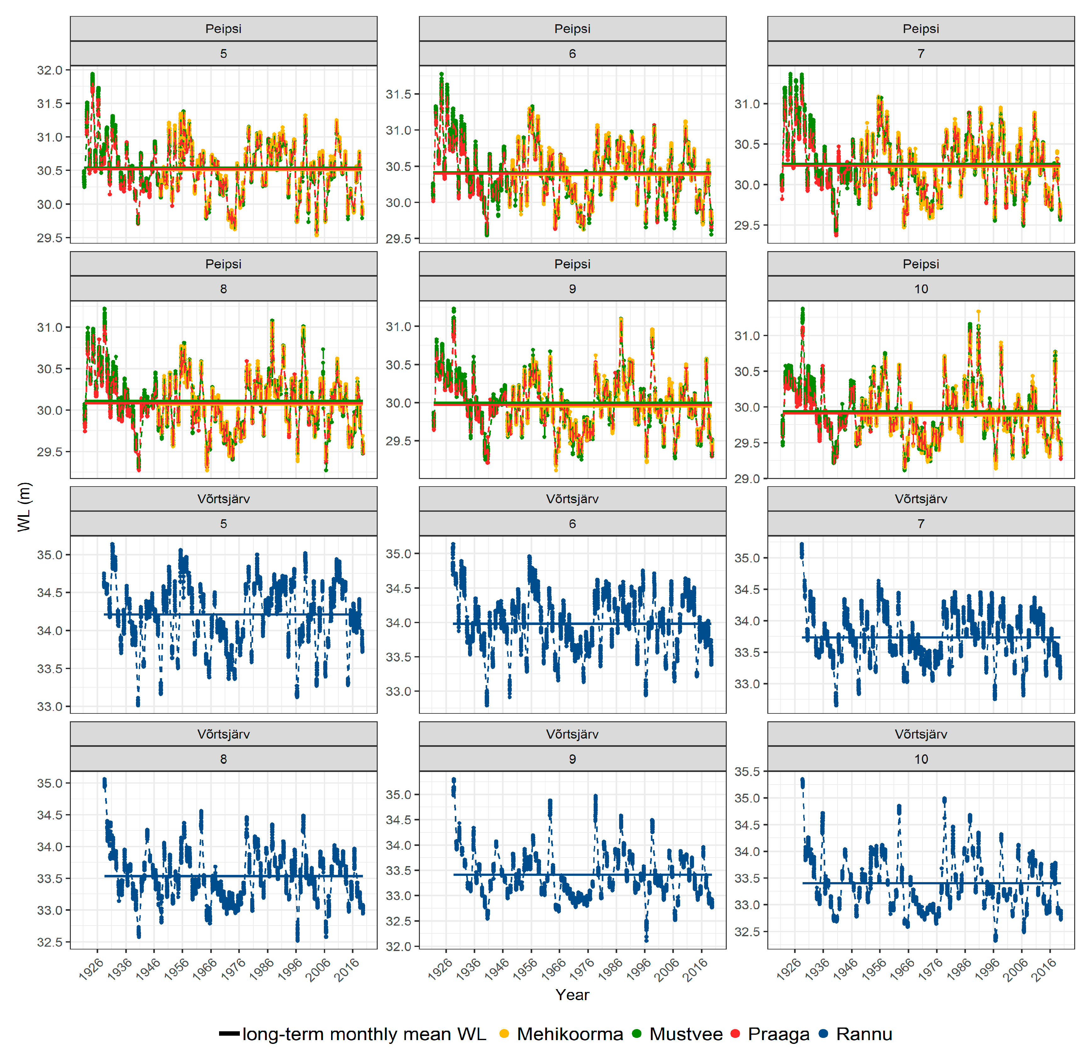
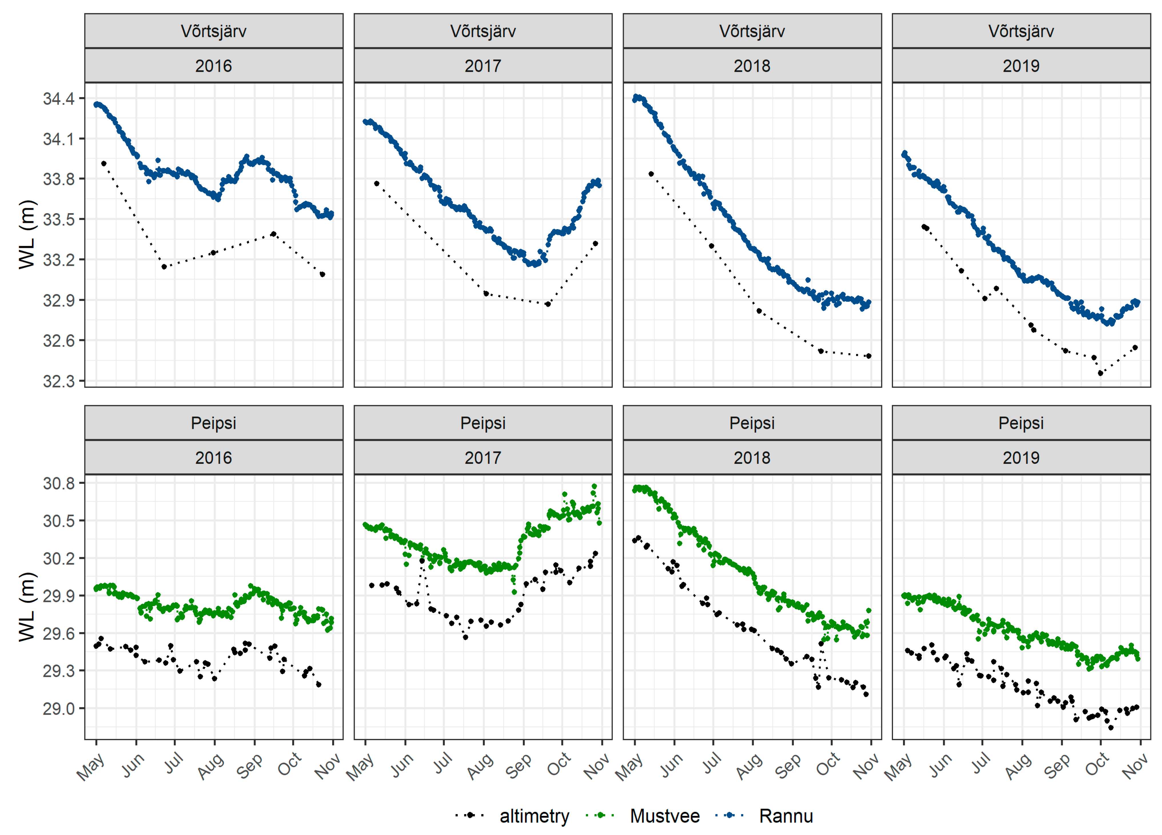
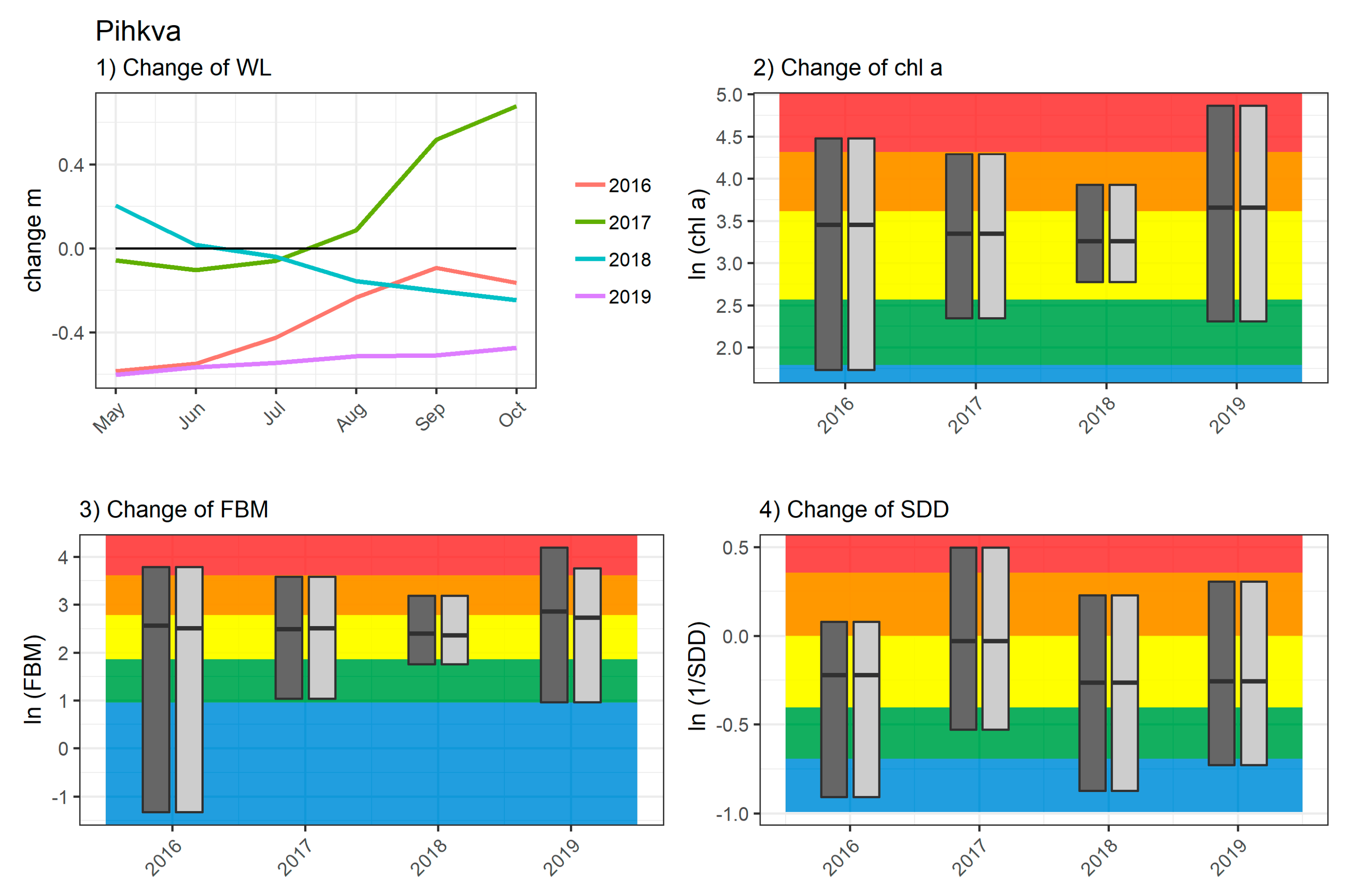
3.1. Inter-Annual Dynamics in Water Level

Comparison of long-term WL measured in three hydrometric stations (Mustvee, Mehikoorma, Praaga) in Peipsi (Figure 2) show similar dynamics and very small spatial differences, e.g., the mean difference between Praaga and Mustvee is 0.02 m, and between Mehikoorma and Mustvee is 0.04 m. In both lakes, the higher and lower WL periods vary similarly and long-term monthly mean WL is highest in May and decreases towards October. While the annual difference can exceed the long-term monthly mean WL (Figure 2) in some years more than 1 meter, its effect is more pronounced in shallower Võrtsjärv (average depth 2.8 m) compared to Peipsi (average depth 7.1 m).
Water levels based on altimetry data and WL measured at the Mustvee hydrometric station show very similar dynamics (Figure 3) with a bias of 0.4 m. Bias corrected Root Mean Standard Error (RMSE) is 0.07 m, whereas the Pearson correlation between WL measured in Mustvee hydrometric station, and derived from altimetry data, is 0.99. Comparison between altimetry data and Rannu hydrometric station in Võrtsjärv shows similar results, with a bias 0.4 m. Bias corrected RMSE is 0.08, whereas the Pearson correlation between WL measured in Rannu hydrometric station and WL, derived from altimetry data, is 0.98. The combination of altimetry data from C2 and S3 missions allows to obtain much more frequent time series, especially since 2018 due to the launch of S3B (Figure 3).

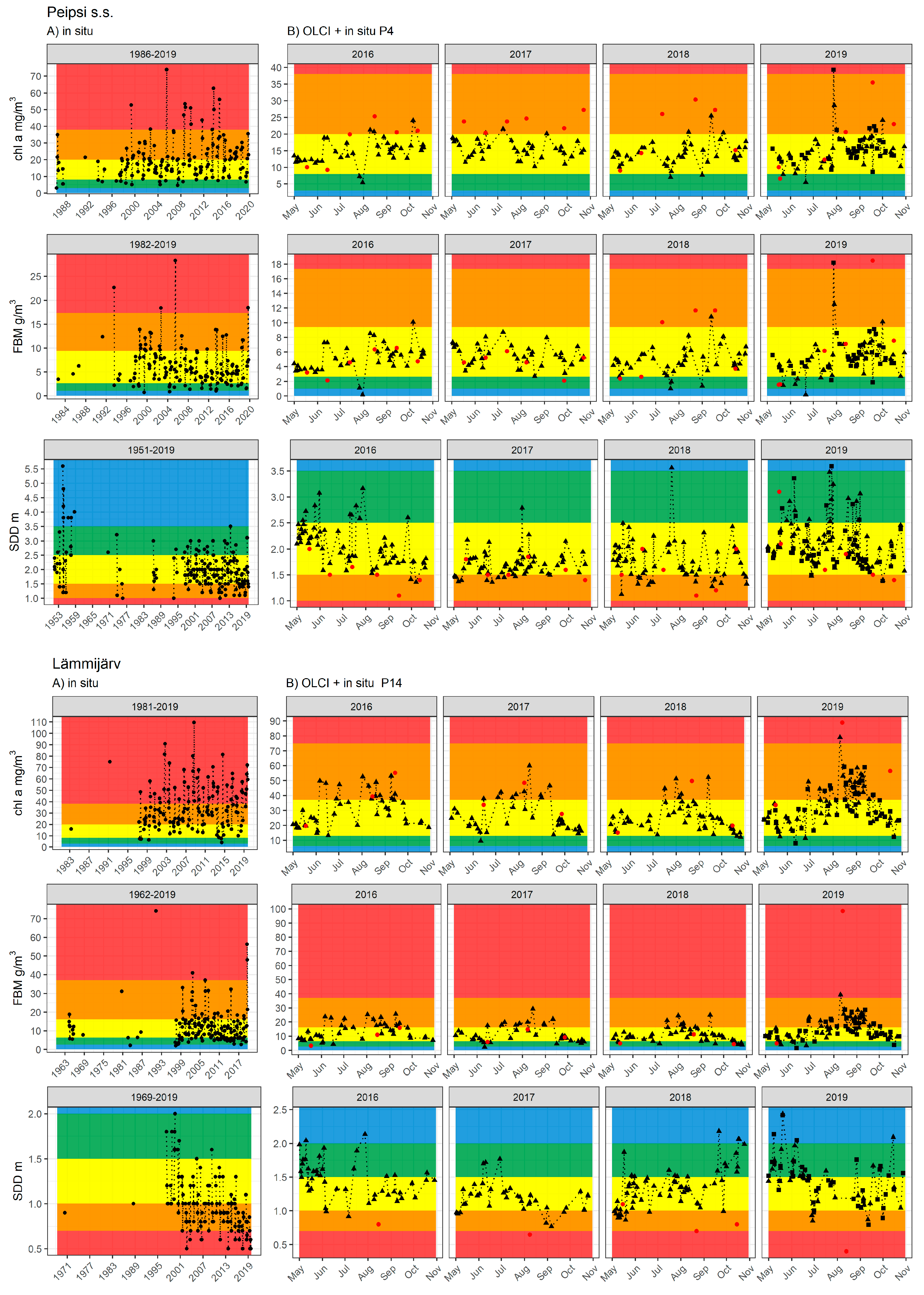
3.2. Inter-Annual Dynamics of Water Quality Parameters

Long-term in situ time series of chl a, FBM, and SDD show variation in seasonal dynamics and pronounced inter-annual differences in Võrtsjärv (Figure 4A). For example, chl a shows increasing trend from 1995 until 2008, then it started to decrease again (Figure 4A). FBM shows increasing trend from the early 2000′s. SDD shows seasonal variation from less than 0.5 to 1.5 m. As WQ parameters are in situ measured once during the vegetation period in Võrtsjärv station named as V2 (Figure 4B), the seasonal dynamics are better obtained with more frequent satellite data resulting on average 50 points, which doubled with S3B launch. This allows to acquire more representative data to analyze the WQ parameters over specific time period and have better knowledge of the seasonal and inter-annual differences.
The dynamics of satellite data corresponded well to in situ measured WQ parameters, showing similar dynamics during vegetation period with a bias for chl a 4.9 ± 11.8 mg/m3, for FBM 2.7 ± 14.2 g/m3, and for SDD was 0.3 ± 0.8 m. Chl a derived from OLCI corresponds to in situ data with Pearson correlation 0.7, whereas FBM 0.6 and SDD 0.4.
Depending on the monitoring system, some areas are not covered with sufficient monitoring frequency (Figure A1 Pihkva A) or include gaps (Figure A1 Peipsi s.s A., Figure A1 Lämmijärv A) in its long-term time series. Satellite data covers these areas 2–3 times per week and with two satellites the amount of data is doubled from 2018.

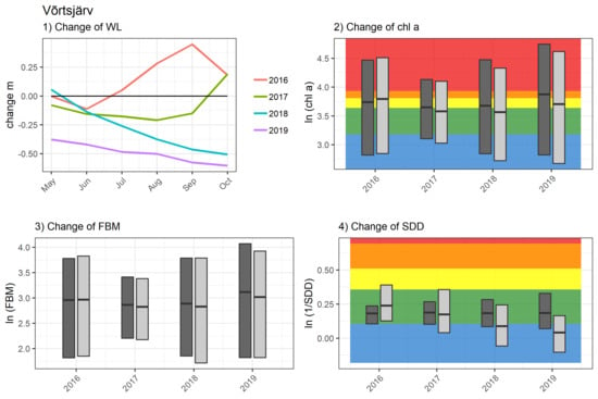
3.3. Correction of chl a, FBM, and SDD Based on the Water Evel

Relationships between WL and WQ parameters vary in both lakes (Table A1). In Võrtsjärv, chl a was significantly related to WL (p < 0.05) in July, August, and October, FBM was significantly related in July, whereas SDD was related in all months (from May to October). In Peipsi s.s., WL was significantly related only with FBM in June and September and in Pihkva, FBM was related in August. In Lämmijärv, chl a was significantly related in July and August, FBM was related in June and SDD in June, July, and August. When the relationship was significant between WL and specific WQ parameter, correction was applied on a daily basis according to the WL value in respect to long-term monthly mean WL. When WL was higher than long-term monthly mean WL, WQ parameter values increased after correction, if the WL was lower, then WQ parameters were corrected to lower values. This changed the mean value of the month, as well as minimum and maximum values.
In Võrtsjärv, WL was higher than long-term monthly mean WL in 2016 (up to 0.3 m) and lower in 2017 until 2019, especially low in 2018 and 2019 towards autumn, when WL was lower by more than 0.5 m (Figure 5). As WL was high in 2016, the mean value of chl a and SDD increased after applying the WL correction, whereas, in 2017 until 2019, mean values decreased. Due to the decrease in mean values, ecological status class of WQ parameters also changed. In 2017 and 2018, the ecological status class of chl a changed from “moderate” to “good”, and in 2019 from “bad” to “moderate”, whereas the ecological status class remained the same in 2016, although mean value of chl a increased. The ecological status class of SDD, changed from “good” to “very good” in 2018 and 2019, when the WL was the lowest compared to long-term monthly mean WL (Figure 5).
In Peipsi, there was less significant relationships between WL and WQ parameters than in Võrtsjärv (Table A1). In Peipsi s.s., there was no statistically significant relationships between WL and WQ parameters, except for FBM in June and September, which only leads to a small change of mean values of FBM (Figure A2 Peipsi s.s. FBM). As WL was lower than long-term monthly mean WL in 2016, 2018, and 2019, mean FBM value slightly decreased without changing the ecological status class. More significant relationships between WL and WQ parameters appeared in Lämmijärv (Figure A2 Lämmijärv), which also changed the ecological status class of SDD. As WL was more than 0.4 m lower than long-term monthly mean WL in 2019, then ecological status class of SDD changed from “moderate” to “good”, and the mean value of SDD in 2016 also decreased. In Pihkva, the amount of in situ data was mostly insufficient for statistical analysis (significant relationship was found only in August for FBM) and therefore, there were no changes in ecological status class estimations of WQ parameters (Figure A2 Pihkva).
As Võrtsjärv and Lämmijärv are shallower than Peipsi s.s., statistically significant relationships between WL and specific WQ parameters tend to occur more frequently there on a monthly basis. More pronounced changes in WL (difference approximately from 0.4 m) from long-term monthly mean WL were influencing not only the mean values of WQ parameters, but even changed the ecological status class from one to another. Smaller changes in WL in respective to long-term monthly mean influenced only the mean values of WQ, not the ecological status class. However, it is still important, considering long-term monitoring of the lake.

4. Discussion

Long-term time series of WQ parameters in lakes are important to obtain information about the seasonal dynamics, their past and present situation and form the basis for future predictions [77,78]. The variety of measured parameters allow the partition of the influences by anthropogenic, as well as natural factors. Moreover, long-term time series help to understand the necessity for current management improvements for the future [79]. Water level as a natural factor, has an impact on lakes ecosystem and on WQ parameters, which in turn have a high impact on the ecological status of lakes [80,81]. Changes in the lake ecosystem influence biota existence and survival complexity in the lake, which affect ecosystem structure and future perspective [82,83,84]. Water level plays an important role in the lake ecosystem, especially in large shallow lakes [85], where monthly WL differences can be highly different from long-term observations, therefore removing WL influence from WQ parameters is beneficial for fair status assessment [62]. This study shows the possibility to create synergy between optical and altimetry data for lakes research, especially in terms of WFD reporting needs. The removal of one natural aspect will improve the estimation of the ecological status class of a lake, which will allow to keep the focus on the anthropogenic changes in the lake ecosystem.
The study shows high variations between seasonal and long-term WL in large and shallow lakes. Low WL periods vary with higher WL periods in both Võrtsjärv and Peipsi, which are caused by variation in precipitation, hydrological inflows, and evaporation in different years [86]. Long-term monthly mean WL decrease, from May towards October, characterizing higher WL after snow and ice melting, and lower WL in summer due to less inflow and higher rate of evaporation during the warm period [86,87]. Not only seasonal temperature and precipitation variability influences WL, but climate change has also direct effect to lake ecosystem [88,89,90,91], which has been even pointed out by The Intergovernmental Panel on Climate Change [92] referring to a global problem. The decrease in WL in some areas is often not compensated by the precipitation, which is caused by the higher annual mean air temperature, which, in turn, causes intensive evaporation and higher water temperature, causing a decrease in ice cover thickness and duration [93,94]. On the other hand, extreme events (flooding, rainfalls, storms, etc.) due to climate change are causing an abrupt increase in the WL in some areas, causing also more apparent WL fluctuations [81,86].
As WL is sensitive to external factors, it is important to monitor it continuously [86,90,95,96,97]. As the number of in situ gauging stations is decreasing due to their cost and maintenance needs, the use of altimetry data becomes an important supplement to measure lake level variations. The use of altimetry has already provided promising results over lakes [10,11,16,50,98,99,100,101,102,103,104,105]. This is confirmed in this study, where a good agreement between the altimetry-based WL and WL measured at hydrometric stations with a correlation up to 0.99 in both lakes, with RMSE for Võrtsjärv 0.07 and for Peipsi 0.08, respectively. By applying measurements from different altimetry satellites the amount of data is increased, hence, providing a better understanding of WL dynamics and its changes [106,107,108]. However, combining data located at different tracks may introduce errors due to unresolved geoid signals, or other effects that causes the lake surface so be spatially different such as wind or land signals near the shoreline, but could be combined when the spatial differences in WL are small inside the water body. For example, comparing WL in Peipsi hydrometric stations, seasonal dynamics of the WL were similar and differences remained between 0.02 and 0.04 m, which shows possible WL homogeneity in the water body. Here, S3 SRAL and C2 SIRAL data were combined to increase the data frequency, but other missions could also have been used. Additionally, S3 and C2 provide SAR mode data in the study area, which give higher along-track resolution than conventional altimetry, with dense C2 spatial tracks suitable for lakes. The continuation of S3 missions, and the recently launched S6 mission, ensure data for future monitoring, which allows to continue developing EO-based applications to monitor WL and its implication for ecosystems and their services.
The possibility to derive certain WQ parameters from satellites helps to collect data more frequently and from places, which are not easily accessible. Satellite data corresponded to in situ data showing correlation 0.7 for chl a and lower than 0.6 for FBM and SDD, whereas bias for chl a was 4.9 ± 11.8 mg/m3, for FBM 2.7 ± 14.2 g/m3, and for SDD 0.3 ± 0.8 m. More data from satellites gives an extra information to in situ data, which enables to detect seasonal dynamics and rapid changes in different parts of a lake, especially in terms of estimating chl a, FBM, SDD based ecological status class. In some cases, satellite data overestimated (Figure 4 Võrtsjärv B SDD, Figure A1 Lämmijärv B SDD) or underestimated (Figure A1 Peipsi s.s. B chl a) in comparison of in situ data. This can be due to spatial differences (point measurement vs. 300 m × 300 m pixel), measurement technique (integral sample vs upper water column captured by satellite), but still, both in situ and EO data show similar trends during the vegetation period and complement each other. Different WQ parameters have been used for estimating ecological status of lakes from satellite data by many authors already for a while [7,25,33,36,41,109], which confirms necessity of this work for WFD.
Based on the long-term in situ data, the study shows significant relationships (p < 0.05) between WL and WQ more frequently in Võrtsjärv than in Peipsi. It is caused by the fact, that Võrtsjärv is shallower than Peipsi and high seasonal WL amplitude affects its biota in greater extent. In addition, the relationships between WL and WQ parameters were more often significant in the shallower parts of Peipsi (e.g., in Lämmjärv). Correcting WQ parameters with WL results in the change of mean annual WQ parameter values and even in changes of their ecological status class. The impact was more pronounced in Võrtsjärv, where WL was much lower than long-term monthly mean WL (approximately from 0.5 m), which did not only decrease the mean value of WQ parameters, but even changed the ecological status estimation to a higher class. As WL has a high impact to WQ parameters and the whole ecosystem, it is encouraging to see that EO data can be used to remove WL effect from data of WQ estimates in large shallow lakes, thus it could be one of the research topics deserving more attention due to its applicability to other large and shallow lakes. Moreover, the variety of past, present, and future satellite missions allows to apply the demonstrated methodology to extend the temporal and also spatial extent of the results. This could be done by combining satellite sensors for WQ, e.g., Environmental Satellite (ENVISAT) Medium Resolution Imaging Spectrometer (MERIS), Moderate Resolution Imaging Spectroradiometer (MODIS) to estimate WQ parameters [35,40,110,111,112,113,114], with Topex Poseidon and Jason mission satellites to estimate WL data [51,104,105,115,116]. Additionally, several databases like Hydroweb [105,117], Database for Hydrological Time Series of Inland Waters (DAHITI) [98,118], Global Reservoirs and Lakes Monitor database (G-REALM) of United States Department of Agriculture (USDA) [119] provide water level data of lakes, whereas Globolakes [120,121] and Climate Change Initiative (CCI) [122] provide data of WQ parameters from different satellites. However, Sentinel missions will provide data at least for 20 years, which gives a possibility to gather continuous data from now.
As sustainable lake ecosystems are essential in the present and in the future, it is important to ensure frequent monitoring system and to develop EO-based approaches to improve monitoring and assessment of the ecological status class of lakes, leading, finally, to the better management of lakes. In situ monitoring is still essential to gather data to monitor the ecosystem, but also it is basis for developing and improving new tools and approaches, while satellite data would support it with better spatial and temporal resolution for certain parameters. Synergy between altimetry and optical data, gives possibility to estimate WL, as well as WQ parameters for more precise analysis. Results of this study show that, WL can have a strong impact on WQ parameters in large shallow lakes, where amplitude in WL change is high. This effect can be corrected with the proposed method to improve the estimation of ecological status class of such lakes.

5. Conclusions

EU WFD obligates European countries to monitor WQ of lakes and estimate their ecological status according to reference condition. The ecological status of lakes is influenced by anthropogenic, as well as by natural factors. To decrease the effect of natural factors, WQ parameters should be corrected for WL in case of shallow lakes with changing WL for more accurate identification of human impact and estimation of ecological status. Traditional monitoring methods give valuable long-term time series, however often with constrained spatial and temporal coverage, while satellites provide more frequent data. Many water quality parameters (e.g., chl a, FBM, and SDD) and WL can be derived using EO based data. The development and validation of EO algorithms allow to create synergy between different types of satellite data which enables to analyze and assess the lake ecosystems and provide complementary information to improve the monitoring and management decisions.
Long-term in situ data show inter-annual and seasonal dynamics of indicators characterizing lake ecosystems. In large and shallow lakes such as Võrtsjärv and Peipsi, amplitude of seasonal WL changes is high (more than 1 m), which influences WQ parameters, especially in shallower Võrtsjärv. The results support previous studies [10,99,101,104] in the fact that WL can be estimated with high accuracy (bias 0.4 m, R 0.99) over lakes with EO data. Correcting WQ parameters with the WL data derived from satellite, the mean values of the parameters and resulting ecological status classes changed in some cases. The highest changes occurred in Võrtsjärv during the years with lower WL compared to the long-term monthly mean. In this case the correction of the values of WQ parameters changed the resulting ecological status to better quality class. Therefore, taking into account the variability of WL and correcting its effect in case of shallow lakes is important to decrease the influence of the natural factors on the assessment of the lakes ecological status class in terms of EU WFD.

Author Contributions

Conceptualization, A.A.-T. and K.A.; methodology, A.A.-T. and K.A.; validation, A.A.-T. and K.A.; formal analysis, A.A.-T. and K.A.; resources, A.A.-T., K.A., K.N., L.T., and K.K.; writing—original draft preparation, A.A.-T.; writing—review and editing, A.A.-T., K.A., K.N., L.T., and K.K.; visualization, A.A.-T.; supervision, K.A., K.N., and L.T. All authors have read and agreed to the published version of the manuscript.

Funding

This research was funded by (1) Estonian Research Council research and development program grant number RITA1/02-52-01; (2) EU’s Horizon 2020 research and innovation program (grant agreement no. 730066, EOMORES) and; (3) Estonian Research Council personal start-up grant named as PSG10 and team grant named as PRG709.

Institutional Review Board Statement

Not applicable.

Informed Consent Statement

Not applicable.

Data Availability Statement

Data available on request.

Acknowledgments

We are grateful to anonymous reviewers for their feedback and suggestions that helped to improve the manuscript. This study was financially supported by (1) the European Regional Development Fund within National Program for Addressing Socio-Economic Challenges through R&D (project named as RITA1 grant number RITA1/02-52-01); (2) European Union’s Horizon 2020 research and innovation program under grant agreement no. 730066; (3) Estonian Research Council grants PSG10 and PRG709. Authors thank people from Centre for Limnology providing in situ water quality data and Estonian Weather Service providing in situ water level data.

Conflicts of Interest

The authors declare no conflict of interest.

Appendix A

Figure A1. Long-term time series of in situ measured chl a, FBM, and SDD in Peipsi s.s., Lämmijärv, and Pihkva (A) and same parameters measured from S3 OLCI (B). Dots indicate in situ measured values. Triangles and squares indicates S3A and S3B values, respectively. Different colors represent ecological status classes according to EU WFD.
Remotesensing 13 00770 g0a1aRemotesensing 13 00770 g0a1b

Appendix B

Table A1. Relationship between in situ measured WL (cm) and water quality parameters from May (5) to October (10), where bold values indicate statistically significant relationships (p < 0.05), N indicates number of observations during the study period and “-” indicates not enough observations for statistical analysis.
ParameterMonthp-ValuerInterceptSlopeN
Võrtsjärv
Ln (chl a)50.12−0.208.76−0.00261
60.67−0.065.85−0.00158
70.01−0.3515.12−0.00357
80.01−0.3114.36−0.00365
90.19−0.179.37−0.00257
100.02−0.3112.17−0.00257
Ln (FBM)50.610.06−0.880.00178
60.48−0.086.83−0.00174
70.01−0.2816.00−0.00476
80.23−0.149.59−0.00276
90.17−0.169.06−0.00278
100.15−0.178.99−0.00270
Ln (1/SDD)50.02−0.244.37−0.00185
60.02−0.276.56−0.00278
70.00−0.418.66−0.00272
80.00−0.5411.46−0.00377
90.00−0.5814.77−0.00478
100.00−0.4810.82−0.00375
Peipsi s.s.
Ln (chl a)50.45−0.159.85−0.00229
60.11−0.3525.58−0.00822
70.880.031.340.00025
80.20−0.2616.39−0.00426
90.13−0.3018.30−0.00527
100.900.031.970.00024
Ln (FBM)50.590.11−5.320.00228
60.00−0.5833.07−0.01122
70.950.010.600.00025
80.52−0.1311.26−0.00326
90.01−0.4833.50−0.01125
100.760.06−1.740.00127
Ln (1/SDD)51.000.00−0.890.00053
60.07−0.275.97−0.00246
70.48−0.092.91−0.00162
80.48−0.113.96−0.00247
90.71−0.061.00−0.00147
100.45−0.111.82−0.00147
Lämmijärv
Ln (chl a)50.33−0.2011.25−0.00326
61.000.002.970.00022
70.00−0.6226.65−0.00822
80.03−0.4623.17−0.00623
90.38−0.2013.54−0.00322
100.45−0.1711.97−0.00321
Ln (FBM)50.54−0.117.21−0.00231
60.04−0.4423.63−0.00722
70.21−0.269.39−0.00225
80.09−0.3423.96−0.00726
90.05−0.4021.75−0.00624
100.20−0.2814.40−0.00423
Ln (1/SDD)50.21−0.274.82−0.00223
60.00−0.6111.25−0.00422
70.01−0.5613.38−0.00421
80.04−0.4312.46−0.00423
90.17−0.318.22−0.00321
100.10−0.378.53−0.00321
Pihkva
Ln (chl a)5-----
6-----
7-----
80.05−0.4727.75−0.00818
9-----
10-----
Ln (FBM)50.96−0.023.140.0007
6-----
7-----
80.00−0.6746.28−0.01417
9-----
10-----
Ln (1/SDD)50.17−0.6419.19−0.0066
60.630.19−10.910.0039
70.310.50−7.500.0026
80.14−0.3414.57−0.00520
90.36−0.4627.64−0.0096
100.26−0.6215.38−0.0055

Appendix C

Figure A2. Water level change from long-term monthly mean WL during the study period in Peipsi s.s., Lämmijärv, and Pihkva (1). Value 0 indicates long-term monthly mean WL. Mean, maximum, and minimum values of water quality parameters are represented on the graphs (24), where dark gray indicates values before and light gray indicates values after applying WL correction. Different colors represent ecological classes according to EU WFD.
Remotesensing 13 00770 g0a2aRemotesensing 13 00770 g0a2b

References

  1. Ritchie, J.C.; Zimba, P.V.; Everitt, J.H. Remote Sensing Techniques to Assess Water Quality. Photogramm. Eng. Remote Sens. 2003, 69, 695–704. [Google Scholar] [CrossRef] [Green Version]
  2. Gray, N.F. Drinking Water Quality. Problems and Solutions; Cambridge University Press: Cambridge, UK, 2008. [Google Scholar]
  3. Munné, A.; Prat, N. Ecological aspects of the Water Framework Directive. In The Water Framework Directive in Catalonia; Generalitat de Catalunya: Barcelona, Spain, 2006; pp. 53–75. [Google Scholar]
  4. Tranvik, L.J.; Downing, J.A.; Cotner, J.B.; Loiselle, S.A.; Striegl, R.G.; Ballatore, T.J.; Dillon, P.; Finlay, K.; Fortino, K.; Knoll, L.B.; et al. Lakes and reservoirs as regulators of carbon cycling and climate. Limnol. Oceanogr. 2009, 54, 2298–2314. [Google Scholar] [CrossRef] [Green Version]
  5. European Comission. WFD 2000/60/EC of the European Parliament and of the Council of 23 October 2000 establishing a framework for Community action in the field of water policy. Off. J. Eur. Parliam. 2000, L327, 1–82. [Google Scholar] [CrossRef]
  6. Ferreira, J.G.; Vale, C.; Soares, C.V.; Salas, F.; Stacey, P.E.; Bricker, S.B.; Silva, M.C.; Marques, J.C. Monitoring of coastal and transitional waters under the E.U. water framework directive. Environ. Monit. Assess. 2007, 135, 195–216. [Google Scholar] [CrossRef] [Green Version]
  7. Arle, J.; Mohaupt, V.; Kirst, I. Monitoring of Surface Waters in Germany under the Water Framework Directive—A Review of Approaches, Methods and Results. Water 2016, 8, 217. [Google Scholar] [CrossRef]
  8. Giardino, C.; Bresciani, M.; Stroppiana, D.; Oggioni, A.; Morabito, G. Optical remote sensing of lakes: An overview on Lake Maggiore. J. Limnol. 2014, 73, 201–214. [Google Scholar] [CrossRef] [Green Version]
  9. Gao, Q.; Makhoul, E.; Escorihuela, M.; Zribi, M.; Quintana Seguí, P.; García, P.; Roca, M. Analysis of Retrackers’ Performances and Water Level Retrieval over the Ebro River Basin Using Sentinel-3. Remote Sens. 2019, 11, 718. [Google Scholar] [CrossRef] [Green Version]
  10. Nielsen, K.; Stenseng, L.; Andersen, O.B.; Villadsen, H.; Knudsen, P. Validation of CryoSat-2 SAR mode based lake levels. Remote Sens. Environ. 2015, 171, 162–170. [Google Scholar] [CrossRef] [Green Version]
  11. Jiang, L.; Schneider, R.; Andersen, O.B.; Bauer-Gottwein, P. CryoSat-2 altimetry applications over rivers and lakes. Water 2017, 9, 211. [Google Scholar] [CrossRef]
  12. Ayana, E.K. Validation of Radar Altimetry Lake Level Data And It’s Application in Water Resource Management. Master’s Thesis, International Institute for Geo-information Science and Earth Observation, Enschede, The Netherlands, 2007. [Google Scholar]
  13. Sheffield, J.; Wood, E.F.; Pan, M.; Beck, H.; Coccia, G.; Serrat-Capdevila, A.; Verbist, K. Satellite Remote Sensing for Water Resources Management: Potential for Supporting Sustainable Development in Data-Poor Regions. Water Resour. Res. 2018, 54, 9724–9758. [Google Scholar] [CrossRef] [Green Version]
  14. Avisse, N.; Tilmant, A.; François Müller, M.; Zhang, H. Monitoring small reservoirs’ storage with satellite remote sensing in inaccessible areas. Hydrol. Earth Syst. Sci. 2017, 21, 6445–6459. [Google Scholar] [CrossRef] [Green Version]
  15. Gholizadeh, M.H.; Melesse, A.M.; Reddi, L. A Comprehensive Review on Water Quality Parameters Estimation Using Remote Sensing Techniques. Sensors 2016, 16, 1298. [Google Scholar] [CrossRef] [Green Version]
  16. Göttl, F.; Dettmering, D.; Müller, F.L.; Schwatke, C. Lake Level Estimation Based on CryoSat-2 SAR Altimetry and Multi-Looked Waveform Classification. Remote Sens. 2016, 8, 885. [Google Scholar] [CrossRef] [Green Version]
  17. Dettmering, D.; Schwatke, C.; Boergens, E.; Seitz, F. Potential of ENVISAT Radar Altimetry for Water Level Monitoring in the Pantanal Wetland. Remote Sens. 2016, 8, 596. [Google Scholar] [CrossRef] [Green Version]
  18. Ismail, K.; Boudhar, A.; Abdelkrim, A.; Mohammed, H.; Mouatassime, S.; Kamal, A.; Driss, E.; Idrissi, E.; Nouaim, W. Evaluating the potential of Sentinel-2 satellite images for water quality characterization of artificial reservoirs: The Bin El Ouidane Reservoir case study (Morocco). Meteorol. Hydrol. Water Manag. 2019, 7, 31–39. [Google Scholar] [CrossRef]
  19. Salmaso, N.; Mosello, R. Limnological research in the deep southern subalpine lakes: Synthesis, directions and perspectives. Adv. Oceanogr. Limnol. 2010, 1, 29–66. [Google Scholar] [CrossRef]
  20. European Commission. Copernicus: New Name for European Earth Observation Programme; European Commission: Brussels, Belgium, 2012. [Google Scholar]
  21. European Commission. Copernicus Programme. Available online: https://www.copernicus.eu/en/about-copernicus/copernicus-brief (accessed on 12 June 2020).
  22. van der Woerd, H.J.; Wernand, M.R. True Colour Classification of Natural Waters with Medium-Spectral Resolution Satellites: SeaWiFS, MODIS, MERIS and OLCI. Sensors 2015, 15, 25663–25680. [Google Scholar] [CrossRef] [Green Version]
  23. Merchant, C.J.; Embury, O.; Bulgin, C.E.; Block, T.; Corlett, G.K.; Fiedler, E.; Good, S.A.; Mittaz, J.; Rayner, N.A.; Berry, D.; et al. Satellite-based time-series of sea-surface temperature since 1981 for climate applications. Sci. Data 2019, 6, 223. [Google Scholar] [CrossRef] [Green Version]
  24. Matthews, M.W. A current review of empirical procedures of remote sensing in Inland and near-coastal transitional waters. Int. J. Remote Sens. 2011, 32, 6855–6899. [Google Scholar] [CrossRef]
  25. Alikas, K.; Kangro, K.; Randoja, R.; Philipson, P.; Asuküll, E.; Pisek, J.; Reinart, A. Satellite-based products for monitoring optically complex inland waters in support of EU Water Framework Directive. Int. J. Remote Sens. 2015, 36, 4446–4468. [Google Scholar] [CrossRef]
  26. Riffler, M.; Lieberherr, G.; Wunderle, S. Lake surface water temperatures of European Alpine lakes (1989–2013) based on the Advanced Very High Resolution Radiometer (AVHRR) 1 km data set. Earth Syst. Sci. Data 2015, 7, 1–17. [Google Scholar] [CrossRef] [Green Version]
  27. Clark, J.M.; Schaeffer, B.A.; Darling, J.A.; Urquhart, E.A.; Johnston, J.M.; Ignatius, A.R.; Myer, M.H.; Loftin, K.A.; Werdell, P.J.; Stumpf, R.P. Satellite monitoring of cyanobacterial harmful algal bloom frequency in recreational waters and drinking water sources. Ecol. Indic. 2017, 80, 84–95. [Google Scholar] [CrossRef]
  28. Leshkevich, G.A.; Nghiem, S.V. Satellite SAR Remote Sensing of Great Lakes Ice Cover, Part 2. Ice Classification and Mapping. J. Great Lakes Res. 2007, 33, 736–750. [Google Scholar] [CrossRef] [Green Version]
  29. Iestyn Woolway, R.; Merchant, C.J. Amplified surface temperature response of cold, deep lakes to inter-annual air temperature variability. Sci. Rep. 2017, 7, 4130. [Google Scholar] [CrossRef] [Green Version]
  30. Duguay, C.R.; Bernier, M.; Gauthier, Y.; Kouraev, A. Remote sensing of lake and river ice. In Remote Sensing of the Cryosphere; Tedesco, M., Ed.; John Wiley & Sons, Ltd.: Hoboken, NJ, USA, 2015; pp. 273–306. ISBN 9781118368909. [Google Scholar]
  31. Simis, S.G.H.; Peters, S.W.M.; Gons, H.J. Remote sensing of the cyanobacterial pigment phycocyanin in turbid inland water. Limnol. Oceanogr. 2005, 50, 237–245. [Google Scholar] [CrossRef]
  32. Papathanasopoulou, E.; Simis, S.; Alikas, K.; Ansper, A.; Anttila, S.; Jenni, A.; Barillé, A.-L.; Barillé, L.; Brando, V.; Bresciani, M.; et al. Satellite-assisted monitoring of water quality to support the implementation of the Water Framework Directive. EOMORES White Pap. 2019, 1–28. [Google Scholar] [CrossRef]
  33. Ansper, A.; Alikas, K. Retrieval of Chlorophyll a from Sentinel-2 MSI Data for the European Union Water Framework Directive Reporting Purposes. Remote Sens. 2019, 11, 64. [Google Scholar] [CrossRef] [Green Version]
  34. Bresciani, M.; Stroppiana, D.; Odermatt, D.; Morabito, G.; Giardino, C. Assessing remotely sensed chlorophyll-a for the implementation of the Water Framework Directive in European perialpine lakes. Sci. Total Environ. 2011, 409, 3083–3091. [Google Scholar] [CrossRef] [Green Version]
  35. Attila, J.; Kauppila, P.; Kallio, K.Y.; Alasalmi, H.; Keto, V.; Bruun, E.; Koponen, S. Applicability of Earth Observation chlorophyll-a data in assessment of water status via MERIS—With implications for the use of OLCI sensors. Remote Sens. Environ. 2018, 212, 273–287. [Google Scholar] [CrossRef]
  36. Gohin, F.; Saulquin, B.; Oger-Jeanneret, H.; Lozac’h, L.; Lampert, L.; Lefebvre, A.; Riou, P.; Bruchon, F. Towards a better assessment of the ecological status of coastal waters using satellite-derived chlorophyll-a concentrations. Remote Sens. Environ. 2008, 112, 3329–3340. [Google Scholar] [CrossRef] [Green Version]
  37. Matthews, M.W.; Bernard, S.; Winter, K. Remote sensing of cyanobacteria-dominant algal blooms and water quality parameters in Zeekoevlei, a small hypertrophic lake, using MERIS. Remote Sens. Environ. 2010, 114, 2070–2087. [Google Scholar] [CrossRef]
  38. Alikas, K.; Kratzer, S. Improved retrieval of Secchi depth for optically-complex waters using remote sensing data. Ecol. Indic. 2017, 77, 218–227. [Google Scholar] [CrossRef]
  39. Alikas, K.; Kratzer, S.; Reinart, A.; Kauer, T.; Paavel, B. Robust remote sensing algorithms to derive the diffuse attenuation coefficient for lakes and coastal waters. Limnol. Oceanogr. Methods 2015, 13, 402–415. [Google Scholar] [CrossRef]
  40. Liu, X.; Lee, Z.; Zhang, Y.; Lin, J.; Shi, K.; Zhou, Y.; Qin, B.; Sun, Z. Remote Sensing of Secchi Depth in Highly Turbid Lake Waters and Its Application with MERIS Data. Remote Sens. 2019, 11, 2226. [Google Scholar] [CrossRef] [Green Version]
  41. Free, G.; Bresciani, M.; Trodd, W.; Tierney, D.; O’Boyle, S.; Plant, C.; Deakin, J. Estimation of lake ecological quality from Sentinel-2 remote sensing imagery. Hydrobiologia 2020, 847, 1423–1438. [Google Scholar] [CrossRef]
  42. Uudeberg, K.; Ansko, I.; Põru, G.; Ansper, A.; Reinart, A. Using Optical Water Types to Monitor Changes in Optically Complex Inland and Coastal Waters. Remote Sens. 2019, 11, 2297. [Google Scholar] [CrossRef] [Green Version]
  43. Soomets, T.; Uudeberg, K.; Jakovels, D.; Zagars, M.; Reinart, A.; Brauns, A.; Kutser, T. Comparison of lake opticalwater types derived from sentinel-2 and sentinel-3. Remote Sens. 2019, 11, 2883. [Google Scholar] [CrossRef] [Green Version]
  44. Xue, K.; Ma, R.; Wang, D.; Shen, M. Optical classification of the remote sensing reflectance and its application in deriving the specific phytoplankton absorption in optically complex lakes. Remote Sens. 2019, 11, 184. [Google Scholar] [CrossRef] [Green Version]
  45. González Vilas, L.; Spyrakos, E.; Torres Palenzuela, J.M. Neural network estimation of chlorophyll a from MERIS full resolution data for the coastal waters of Galician rias (NW Spain). Remote Sens. Environ. 2011, 115, 524–535. [Google Scholar] [CrossRef]
  46. Odermatt, D.; Pomati, F.; Pitarch, J.; Carpenter, J.; Kawka, M.; Schaepman, M.; Wüest, A. MERIS observations of phytoplankton blooms in a stratified eutrophic lake. Remote Sens. Environ. 2012, 126, 232–239. [Google Scholar] [CrossRef]
  47. Ioannou, I.; Gilerson, A.; Gross, B.; Moshary, F.; Ahmed, S. Deriving ocean color products using neural networks. Remote Sens. Environ. 2013, 134, 78–91. [Google Scholar] [CrossRef]
  48. Fink, G.; Burke, S.; Simis, S.G.H.; Kangur, K.; Kutser, T.; Mulligan, M. Management Options to Improve Water Quality in Lake Peipsi: Insights from Large Scale Models and Remote Sensing. Water Resour. Manag. 2020, 34, 2241–2254. [Google Scholar] [CrossRef] [Green Version]
  49. Gitelson, A.A.; Dall’Olmo, G.; Moses, W.; Rundquist, D.C.; Barrow, T.; Fisher, T.R.; Gurlin, D.; Holz, J. A simple semi-analytical model for remote estimation of chlorophyll-a in turbid waters: Validation. Remote Sens. Environ. 2008, 112, 3582–3593. [Google Scholar] [CrossRef]
  50. Nielsen, K.; Stenseng, L.; Andersen, O.B.; Knudsen, P. The Performance and Potentials of the CryoSat-2 SAR and SARIn Modes for Lake Level Estimation. Water 2017, 9, 374. [Google Scholar] [CrossRef]
  51. Troitskaya, Y.I.; Rybushkina, G.V.; Soustova, I.A.; Balandina, G.N.; Lebedev, S.A.; Kostyanoi, A.G.; Panyutin, A.A.; Filina, L.V. Satellite Altimetry of Inland Water Bodies. Water Resour. 2012, 39, 169–185. [Google Scholar] [CrossRef]
  52. Fernandes, M.J.; Lázaro, C.; Nunes, A.L.; Scharroo, R. Atmospheric corrections for altimetry studies over inland water. Remote Sens. 2014, 6, 4952–4997. [Google Scholar] [CrossRef] [Green Version]
  53. Leira, M.; Cantonati, M. Effects of water-level fluctuations on lakes: An annotated bibliography. Hydrobiologia 2008, 613, 171–184. [Google Scholar] [CrossRef]
  54. Wang, X.L.; Lu, Y.L.; Han, J.Y.; He, G.Z.; Wang, T.Y. Identification of anthropogenic influences on water quality of rivers in Taihu watershed. J. Environ. Sci. 2007, 19, 475–481. [Google Scholar] [CrossRef]
  55. Nõges, P.; Van De Bund, W.; Cardoso, A.C.; Heiskanen, A.S. Impact of climatic variability on parameters used in typology and ecological quality assessment of surface waters—Implications on the Water Framework Directive. Hydrobiologia 2007, 584, 373–379. [Google Scholar] [CrossRef]
  56. Koff, T.; Vandel, E.; Marzecová, A.; Avi, E.; Mikomägi, A. Assessment of the effect of anthropogenic pollution on the ecology of small shallow lakes using the palaeolimnological approach. Est. J. Earth Sci. 2016, 65, 221–233. [Google Scholar] [CrossRef]
  57. Khatri, N.; Tyagi, S. Influences of natural and anthropogenic factors on surface and groundwater quality in rural and urban areas. Front. Life Sci. 2015, 8, 23–39. [Google Scholar] [CrossRef]
  58. Wang, M.; Cheng, W.; Huang, J.; Shi, L.; Yu, B. Effects of water-level on water quality of reservoir in numerical simulated experiments. Chem. Eng. Trans. 2016, 51, 733–738. [Google Scholar] [CrossRef]
  59. Chen, M.Q.; Li, Y.; Li, K.F.; Li, R.; Li, J. Effects of water-level decline on water quality of reservoir. Sichuan Daxue Xuebao (Gongcheng Kexue Ban)/J. Sichuan Univ. Eng. Sci. Ed. 2012, 44, 32–36. [Google Scholar]
  60. Nõges, P.; Nõges, T.; Laas, A. Climate-related changes of phytoplankton seasonality in large shallow Lake Võrtsjärv, Estonia. Aquat. Ecosyst. Health Manag. 2010, 13, 154–163. [Google Scholar] [CrossRef]
  61. Nõges, T.; Nõges, P.; Laugaste, R. Water level as the mediator between climate change and phytoplankton composition in a large shallow temperate lake. In Hydrobiologia; Springer: Dordrecht, The Netherlands, 2003; Volume 506–509, pp. 257–263. [Google Scholar]
  62. Tuvikene, L.; Nõges, T.; Nõges, P. Why do phytoplankton species composition and “traditional” water quality parameters indicate different ecological status of a large shallow lake? Hydrobiologia 2011, 660, 3–15. [Google Scholar] [CrossRef]
  63. Nõges, T.; Nõges, P. The effect of extreme water level decrease on hydrochemistry and phytoplankton in shallow eutrophic lake. Hydrobiologia 1999, 408–409, 277–283. [Google Scholar] [CrossRef]
  64. Ministry of Environment. Pinnaveekogumite Moodustamise Kord ja Nende Pinnaveekogumite Nimestik, Mille Seisundiklass Tuleb Määrata, Pinnaveekogumite Seisundiklassid ja Seisundiklassidele Vastavad Kvaliteedinäitajate Väärtused Ning Seisundiklasside Määramise kord-RT I. 25 November 2010. Available online: https://www.riigiteataja.ee/akt/125112010015 (accessed on 3 September 2020).
  65. Keskkonnaministeerium. Keskkonnaseire Infrosüsteem. Available online: https://kese.envir.ee/kese/listProgramAndPublicReport.action (accessed on 27 February 2020).
  66. Mäemets, H.; Laugaste, R.; Palmik, K.; Haldna, M. Response of primary producers to water level fluctuations of Lake Peipsi. Proc. Est. Acad. Sci. 2018, 67, 231–245. [Google Scholar] [CrossRef]
  67. Nõges, P.; Nõges, T. Indicators and criteria to assess ecological status of the large shallow temperate polymictic lakes Peipsi (Estonia/Russia) and Võrtsjärv (Estonia). Boreal Environ. Res. 2006, 11, 67–80. [Google Scholar]
  68. Eesti Ilmateenistus. Hydrological Measurements. Available online: http://www.ilmateenistus.ee/ilmatarkus/mootetehnika/hudroloogiliste-vaatluste-mootetehnika/ (accessed on 9 March 2020).
  69. Ellmann, A.; Märdla, S.; Oja, T. The 5 mm geoid model for Estonia computed by the least squares modified Stokes’s formula. Surv. Rev. 2020, 52, 352–372. [Google Scholar] [CrossRef]
  70. Republic of Estonia Environment Agency. Annex 4. National Environmental Monitoring Program Surface Water Monitoring SUB-Program; Republic of Estonia Environment Agency: Tallinn, Estonia, 2019. [Google Scholar]
  71. Jeffrey, S.W.; Humphrey, G.F. New spectrophotometric equations for determining chlorophylls a, b, c1 and c2 in higher plants, algae and natural phytoplankton. Biochem. Physiol. Pflanz. 1975, 167, 191–194. [Google Scholar] [CrossRef]
  72. Utermöhl, H. Zur Vervollkommnung der quantitativen Phytoplankton-Methodik. Int. Vereinigung für Theor. Angew. Limnol. Mitt. 1958, 9, 1–38. [Google Scholar] [CrossRef]
  73. Respublic of Estonia Land Board. ESTHub Processing Platform. Available online: https://ehcalvalus.maaamet.ee/calest/calvalus.jsp (accessed on 10 December 2019).
  74. Alikas, K.; Kangro, K.; Reinart, A. Detecting cyanobacterial blooms in large North European lakes using the Maximum Chlorophyll Index. Oceanologia 2010, 52, 237–257. [Google Scholar] [CrossRef] [Green Version]
  75. Gower, J.; King, S.; Borstad, G.; Brown, L. Use of the 709 nm band of meris to detect intense plankton blooms and other conditions in coastal waters. Int. J. Remote Sens. 2005, 26, 2005–2012. [Google Scholar] [CrossRef]
  76. Villadsen, H.; Andersen, O.B.; Stenseng, L.; Nielsen, K.; Knudsen, P. CryoSat-2 altimetry for river level monitoring—Evaluation in the Ganges-Brahmaputra River basin. Remote Sens. Environ. 2015, 168, 80–89. [Google Scholar] [CrossRef]
  77. Taheri Tizro, A.; Ghashghaie, M.; Georgiou, P.; Voudouris, K. Time series analysis of water quality parameters. J. Appl. Res. Water Wastewater 2014, 1, 43–52. [Google Scholar]
  78. Monteiro, M.; Costa, M. A time series model comparison for monitoring and forecasting water quality variables. Hydrology 2018, 5, 37. [Google Scholar] [CrossRef] [Green Version]
  79. Wang, F.; Wang, X.; Zhao, Y.; Yang, Z.F. Long-term water quality variations and chlorophyll a simulation with an emphasis on different hydrological periods in Lake Baiyangdian, Northern China. J. Environ. Inform. 2012, 20, 90–102. [Google Scholar] [CrossRef]
  80. Wantzen, K.M.; Rothhaupt, K.-O.; Mörtl, M.; Cantonati, M.; László, G.; Fischer, P. Ecological Effects of Water-Level Fluctuations in Lakes; Springer: Dordrecht, The Netherlands, 2008. [Google Scholar]
  81. Gownaris, N.J.; Rountos, K.J.; Kaufman, L.; Kolding, J.; Lwiza, K.M.M.; Pikitch, E.K. Water level fluctuations and the ecosystem functioning of lakes. J. Great Lakes Res. 2018, 44, 1154–1163. [Google Scholar] [CrossRef]
  82. Maihemuti, B.; Aishan, T.; Simayi, Z.; Alifujiang, Y.; Yang, S. Temporal Scaling of Water Level Fluctuations in Shallow Lakes and Its Impacts on the Lake Eco-Environments. Sustainability 2020, 12, 3541. [Google Scholar] [CrossRef]
  83. Liu, X.; Yang, Z.; Yuan, S.; Wang, H. A novel methodology for the assessment of water level requirements in shallow lakes. Ecol. Eng. 2017, 102, 31–38. [Google Scholar] [CrossRef]
  84. Stefanidis, K.; Papastergiadou, E. Effects of a long term water level reduction on the ecology and water quality in an eastern Mediterranean lake. Knowl. Manag. Aquat. Ecosyst. 2013, 411. [Google Scholar] [CrossRef] [Green Version]
  85. Coops, H.; Beklioglu, M.; Crisman, T.L. The role of water-level fluctuations in shallow lake ecosystems—Workshop conclusions. Hydrobiologia 2003, 506–509, 23–27. [Google Scholar] [CrossRef]
  86. Zohary, T.; Ostrovsky, I. Ecological impacts of excessive water level fluctuations in stratified freshwater lakes. Inl. Waters 2011, 1, 47–59. [Google Scholar] [CrossRef]
  87. Górniak, A.; Piekarski, K. Seasonal and Multiannual Changes of Water Levels in Lakes of Northeastern Poland. Pol. J. Environ. Stud. 2002, 11, 349–354. [Google Scholar]
  88. Jeppesen, E.; Meerhoff, M.; Davidson, T.A.; Trolle, D.; Søndergaard, M.; Lauridsen, T.L.; Beklioǧlu, M.; Brucet, S.; Volta, P.; González-Bergonzoni, I.; et al. Climate change impacts on lakes: An integrated ecological perspective based on a multi-faceted approach, with special focus on shallow lakes. J. Limnol. 2014, 73, 84–107. [Google Scholar] [CrossRef] [Green Version]
  89. Mooij, W.M.; Hülsmann, S.; De Senerpont Domis, L.N.; Nolet, B.A.; Bodelier, P.L.E.; Boers, P.C.M.; Dionisio Pires, L.M.; Gons, H.J.; Ibelings, B.W.; Noordhuis, R.; et al. The impact of climate change on lakes in the Netherlands: A review. Aquat. Ecol. 2005, 39, 381–400. [Google Scholar] [CrossRef]
  90. Torabi Haghighi, A.; Kløve, B. A sensitivity analysis of lake water level response to changes in climate and river regimes. Limnologica 2015, 51, 118–130. [Google Scholar] [CrossRef]
  91. Whitehead, P.G.; Wilby, R.L.; Battarbee, R.W.; Kernan, M.; Wade, A.J. A review of the potential impacts of climate change on surface water quality. Hydrol. Sci. J. 2009, 54, 101–123. [Google Scholar] [CrossRef]
  92. Oppenheimer, M.; Glavovic, B.C.; Hinkel, J.; van de Wal, R.; Magnan, A.K.; Abd-Elgawad, A.; Cai, R.; Cifuentes-Jara, M.; DeConto, R.M.; Ghosh, T.; et al. Sea Level Rise and Implications for Low-Lying Islands, Coasts and Communities. In IPCC Special Report on the Ocean and Cryosphere in a Changing Climate; Pörtner, H.-O., Roberts, D.C., Masson-Delmotte, V., Zhai, P., Tignor, M., Poloczanska, E., Mintenbeck, K., Alegría, A., Nicolai, M., Okem, A., et al., Eds.; IPCC: Geneva, Switzerland, 2019. [Google Scholar]
  93. Vincent, W.F. Effects of Climate Change on Lakes. In Encyclopedia of Inland Waters; Elsvier: Amsterdam, The Netherlands, 2009; pp. 55–60. ISBN 9780123706263. [Google Scholar]
  94. Kiani, T.; Ramesht, M.H.; Maleki, A.; Safakish, F. Analyzing the Impacts of Climate Change on Water Level Fluctuations of Tashk and Bakhtegan Lakes and Its Role in Environmental Sustainability. Open J. Ecol. 2017, 7, 158–178. [Google Scholar] [CrossRef] [Green Version]
  95. Fan, Z.; Wang, Z.; Li, Y.; Wang, W.; Tang, C.; Zeng, F. Water Level Fluctuation under the Impact of Lake Regulation and Ecological Implication in Huayang Lakes, China. Water 2020, 12, 702. [Google Scholar] [CrossRef] [Green Version]
  96. Nhu, V.-H.; Mohammadi, A.; Shahabi, H.; Shirzadi, A.; Al-Ansari, N.; Ahmad, B.B.; Chen, W.; Khodadadi, M.; Ahmadi, M.; Khosravi, K.; et al. Monitoring and Assessment of Water Level Fluctuations of the Lake Urmia and Its Environmental Consequences Using Multitemporal Landsat 7 ETM + Images. Int. J. Environ. Res. Public Health 2020, 17, 4210. [Google Scholar] [CrossRef] [PubMed]
  97. Jalili, S.; Hamidi, S.A.; Namdar Ghanbari, R. Climate variability and anthropogenic effects on Lake Urmia water level fluctuations, northwestern Iran. Hydrol. Sci. J. 2016, 61, 1759–1769. [Google Scholar] [CrossRef] [Green Version]
  98. Schwatke, C.; Dettmering, D.; Bosch, W.; Seitz, F. DAHITI—An innovative approach for estimating water level time series over inland waters using multi-mission satellite altimetry. Hydrol. Earth Syst. Sci. 2015, 19, 4345–4364. [Google Scholar] [CrossRef] [Green Version]
  99. Berry, P.A.M.; Garlick, J.D.; Freeman, J.A.; Mathers, E.L. Global inland water monitoring from multi-mission altimetry. Geophys. Res. Lett. 2005, 32, 16. [Google Scholar] [CrossRef]
  100. Liibusk, A.; Kall, T.; Rikka, S.; Uiboupin, R.; Suursaar, Ü.; Tseng, K.H. Validation of copernicus sea level altimetry products in the baltic sea and estonian lakes. Remote Sens. 2020, 12, 4062. [Google Scholar] [CrossRef]
  101. Nielsen, K.; Andersen, O.B.; Ranndal, H. Validation of sentinel-3a based lake level over US and Canada. Remote Sens. 2020, 12, 2835. [Google Scholar] [CrossRef]
  102. Crétaux, J.F.; Bergé-Nguyen, M.; Calmant, S.; Jamangulova, N.; Satylkanov, R.; Lyard, F.; Perosanz, F.; Verron, J.; Montazem, A.S.; Guilcher, G.L.; et al. Absolute calibration or validation of the altimeters on the Sentinel-3A and the Jason-3 over Lake Issykkul (Kyrgyzstan). Remote Sens. 2018, 10, 1679. [Google Scholar] [CrossRef] [Green Version]
  103. Birkett, C.M. Radar altimetry: A new concept in monitoring lake level changes. Eos Trans. Am. Geophys. Union 1994, 75, 273–275. [Google Scholar] [CrossRef]
  104. Crétaux, J.F.; Birkett, C. Lake studies from satellite radar altimetry. Comptes Rendus-Geosci. 2006, 338, 1098–1112. [Google Scholar] [CrossRef]
  105. Crétaux, J.F.; Jelinski, W.; Calmant, S.; Kouraev, A.; Vuglinski, V.; Bergé-Nguyen, M.; Gennero, M.C.; Nino, F.; Abarca Del Rio, R.; Cazenave, A.; et al. SOLS: A lake database to monitor in the Near Real Time water level and storage variations from remote sensing data. Adv. Space Res. 2011, 47, 1497–1507. [Google Scholar] [CrossRef]
  106. Song, C.; Ye, Q.; Sheng, Y.; Gong, T. Combined ICESat and CryoSat-2 Altimetry for Accessing Water Level Dynamics of Tibetan Lakes over 2003–2014. Water 2015, 7, 4685–4700. [Google Scholar] [CrossRef] [Green Version]
  107. Wu, Y.J.; Qiao, G.; Li, H.W. Water Level Changes Of Nam-Co Lake Based On Satellite Altimetry Data Series. Int. Arch. Photogramm. Remote Sens. Spatial Inf. Sci. 2017, XLII-2/W7, 1555–1560. [Google Scholar] [CrossRef] [Green Version]
  108. Li, P.; Li, H.; Chen, F.; Cai, X. Monitoring long-term lake level variations in middle and lower yangtze basin over 2002-2017 through integration of multiple satellite altimetry datasets. Remote Sens. 2020, 12, 1448. [Google Scholar] [CrossRef]
  109. Chen, Q.; Zhang, Y.; Ekroos, A.; Hallikainen, M. The role of remote sensing technology in the EU water framework directive (WFD). Environ. Sci. Policy 2004, 7, 267–276. [Google Scholar] [CrossRef]
  110. Moses, W.J.; Gitelson, A.A.; Berdnikov, S.; Povazhnyy, V. Estimation of chlorophyll-a concentration in case II waters using MODIS and MERIS data—Successes and challenges. Environ. Res. Lett. 2009, 4, 045005. [Google Scholar] [CrossRef] [Green Version]
  111. Salem, S.I.; Strand, M.H.; Higa, H.; Kim, H.; Kazuhiro, K.; Oki, K.; Oki, T. Evaluation of MERIS Chlorophyll-a Retrieval Processors in a Complex Turbid Lake Kasumigaura over a 10-Year Mission. Remote Sens. 2017, 9, 1022. [Google Scholar] [CrossRef] [Green Version]
  112. Wozniak, M.; Bradtke, K.M.; Krezel, A. Comparison of satellite chlorophyll a algorithms for the Baltic Sea. J. Appl. Remote Sens. 2014, 8, 083605. [Google Scholar] [CrossRef] [Green Version]
  113. Chavula, G.; Brezonik, P.; Thenkabail, P.; Johnson, T.; Bauer, M. Estimating chlorophyll concentration in Lake Malawi from MODIS satellite imagery. Phys. Chem. Earth 2009, 34, 755–760. [Google Scholar] [CrossRef]
  114. Wu, M.; Zhang, W.; Wang, X.; Luo, D. Application of MODIS satellite data in monitoring water quality parameters of Chaohu Lake in China. Environ. Monit. Assess. 2009, 148, 255–264. [Google Scholar] [CrossRef]
  115. Zhang, J.; Xu, K.; Yang, Y.; Qi, L.; Hayashi, S.; Watanabe, M. Measuring water storage fluctuations in Lake Dongting, China, by Topex/Poseidon satellite altimetry. Environ. Monit. Assess. 2006, 115, 23–37. [Google Scholar] [CrossRef]
  116. Birkett, C.M. The contribution of TOPEX/POSEIDON to the global monitoring of climatically sensitive lakes. J. Geophys. Res. 1995, 100, 25179–25204. [Google Scholar] [CrossRef]
  117. Hydroweb. Available online: http://hydroweb.theia-land.fr/ (accessed on 1 February 2021).
  118. Deutsches Geodätisches Forschungsinstitut der Technischen Universität München Database for Hydrological Time Series of Inland Waters. Available online: https://dahiti.dgfi.tum.de/en/ (accessed on 1 February 2021).
  119. Global Reservoirs and Lakes Monitor (G-REALM). Available online: https://ipad.fas.usda.gov/cropexplorer/global_reservoir/ (accessed on 1 February 2021).
  120. Politi, E.; MacCallum, S.; Cutler, M.E.J.; Merchant, C.J.; Rowan, J.S.; Dawson, T.P. Selection of a network of large lakes and reservoirs suitable for global environmental change analysis using Earth Observation. Int. J. Remote Sens. 2016, 37, 3042–3060. [Google Scholar] [CrossRef] [Green Version]
  121. Globolakes. Available online: http://www.globolakes.ac.uk/index.html (accessed on 1 February 2021).
  122. Sathyendranath, S.; Brewin, R.J.W.; Brockmann, C.; Brotas, V.; Calton, B.; Chuprin, A.; Cipollini, P.; Couto, A.B.; Dingle, J.; Doerffer, R.; et al. An ocean-colour time series for use in climate studies: The experience of the ocean-colour climate change initiative (OC-CCI). Sensors 2019, 19, 4285. [Google Scholar] [CrossRef] [Green Version]
Figure 1. Locations of in situ stations in Võrtsjärv (Vx) and Peipsi (Px). Peipsi consists of three parts: Peipsi s.s. (light purple), Lämmijärv (pink), Pihkva (light green); Võrtsjärv is colored as orange. Buffers of 1 and 2 km from the shore are created for Võrtsjärv and Peipsi respectively. Sentinel-3- altimetry tracks are shown in light blue, whereas Cryosat-2 tracks are shown in brown. Locations of hydrometric stations are numbered as 1 Rannu-Jõesuu (blue), 2 Mustvee (green), 3 Praaga (yellow), 4 Mehikoorma (red).
Remotesensing 13 00770 g001
Figure 2. Long-term water level (WL) in Rannu, Mustvee, Praaga, and Mehikoorma hydrometric stations from May (5) to October (10). Long-term monthly mean WL is showed in solid line.
Remotesensing 13 00770 g002
Figure 3. Water level (WL) measured in Mustvee and Rannu hydrometric stations from May to October. WL derived from altimetry data (S3A, S3B, C2).
Remotesensing 13 00770 g003
Figure 4. Long-term time series of in situ measured chl a, FBM, and SDD in Võrtsjärv in station named as V2 (A) and the same parameters measured from S3 Ocean and Land Color Instrument (OLCI) (B). Dots indicate in situ measured values. Triangles and squares indicate S3A and S3B values, respectively. Different colors represent ecological status classes according to European Union (EU) WFD, while FBM is not considered as important parameter to assess the ecological status in Võrtsjärv according to the WFD.
Remotesensing 13 00770 g004
Figure 5. Water level change from long-term monthly mean WL during study period in Võrtsjärv (1). Value 0 indicates long-term monthly mean WL. Mean, maximum and minimum values of EO-derived WQ parameters are represented on the graphs (24), where dark gray indicates values before and light gray indicates values after applying WL correction. Different colors represent ecological status classes according to EU WFD.
Remotesensing 13 00770 g005
Table 1. Thresholds for chlorophyll a (chl a) (mg/m3), phytoplankton biomass (FBM) (g/m3) and Secchi disk depth (SDD) (m) estimating ecological status class in Võrtsjärv and Peipsi according to Estonian regulation of Water Act [64]. Each color represents ecological status class defined by Water Framework Directive (WFD) [5] and the range of measured values for each parameter during the study period from both lakes are shown in the last column, whereas the number in the brackets indicates average of the measured values.
Very GoodGoodModerateBadVery BadStudy Site 2016–2019
Võrtsjärv
Chl a (mg/m3)≤24>24–38>38–45>45–51>515–81 (33)
FBM (g/m³)
SDD (m)≥0.9<0.9–0.7<0.7–0.6<0.6–0.5<0.50.4–2.15 (0.9)
Peipsi
Chl a (mg/m3)≤3 (Peipsi s.s.)
≤6 (Lämmijärv, Pihkva)
>3–8 (Peipsi s.s.)
>6–13 (Lämmijärv, Pihkva)
>8–20 (Peipsi s.s.)
>13–37 (Lämmijärv, Pihkva)
>20–38 (Peipsi s.s.)
>37–75 (Lämmijärv, Pihkva)
>38 (Peipsi s.s.)
>75 (Lämmijärv, Pihkva)
5–89 (19) (Peipsi s.s.) 4–90 (46) (Lämmijärv, Pihkva)
FBM (g/m³)≤1 (Peipsi s.s.)
≤2.6 (Lämmijärv, Pihkva)
>1–2.6 (Peipsi s.s.)
>2.6–6.4 (Lämmijärv, Pihkva)
>2.6–9.4 (Peipsi s.s.)
>6.4–16.1 (Lämmijärv, Pihkva)
>9.4–17.3 (Peipsi s.s.)
>16.1–37 (Lämmijärv, Pihkva)
>17.3 (Peipsi s.s.)
>37 (Lämmijärv, Pihkva)
1.4–98.5 (7.1) (Peipsi s.s.) 2.0–74.4 (18.6) (Lämmijärv, Pihkva)
SDD (m)≥3.5 (Peipsi s.s.)
≥2.0 (Lämmijärv, Pihkva)
<3.5–2.5 (Peipsi s.s.)
<2.0–1.5 (Lämmijärv, Pihkva)
<2.5–1.5 (Peipsi s.s.)
<1.5–1.0 (Lämmijärv, Pihkva)
<1.5–1.0 (Peipsi s.s.)
<1.0–0.7 (Lämmijärv, Pihkva)
<1.0 (Peipsi s.s.)
<0.7 (Lämmijärv, Pihkva)
0.12–3.1 (1.0) (Peipsi s.s.) 0.13–1.1 (0.5) (Lämmijärv, Pihkva)
Publisher’s Note: MDPI stays neutral with regard to jurisdictional claims in published maps and institutional affiliations.

