Abstract
This study investigates the impact of digital transactions on sustainable economic growth in Turkey, utilizing a vector autoregressive (VAR) model and quarterly data from 2006 to 2023. The results indicate a positive long-term association between digital payments and GDP. Granger causality tests and impulse response functions suggest a bidirectional relationship, highlighting mutual reinforcement between economic activity and digital financial adoption. The study also investigates three potential transmission channels linking digital payments to economic performance: household consumption, productivity, and financial intermediation. Evidence shows that digital payments are associated with increased consumption and financial sector activity, while the link to productivity is less conclusive. These findings imply that policymakers should prioritize digital financial infrastructure development and enhance regulatory frameworks to promote inclusive and sustainable economic growth.
1. Introduction
The growing integration of sophisticated technological developments in modern society has enabled seamless, secure, convenient, and cost-effective financial transactions. Digital payment systems have expanded access to banking services and e-commerce, facilitated trade, reduced transaction costs, and enhanced transparency, thereby boosting productivity and helping to curb corruption. User adoption and preference for these technologies have surged in the last decade, reflecting a growing trend driven by both technological progress and evolving consumer habits [1]. The COVID-19 pandemic has further accelerated this shift by spurring innovations in the sector, including card payment systems, contactless payments, and wearable payment technologies.
Studies that examine the impact of digital payments on the real economy and the financial sector have flourished in recent years. These studies have focused on a number of macroeconomic and financial variables, including the velocity of money [2,3,4], money demand [5], inflation [6], informal economy [7,8] corruption [9], financial stability [10], consumer demand [11,12], and economic growth [13,14,15,16,17,18].
Despite extensive research on the determinants of economic growth, the role played by digital banking is a recent phenomenon. Existing studies overwhelmingly have a cross-country context based on the analysis of panel data. Single-country studies are quite rare. Although both approaches have their own advantages, country-specific studies can be more valuable in certain contexts for several reasons. Countries differ in their economic structure, financial systems, and social norms. Panel studies assume some level of homogeneity across countries, which can lead to misleading conclusions if key structural differences are not accounted for. A country-focused study can provide a richer qualitative and quantitative analysis of causal relationships.
This study seeks to expand on this body of work in three directions. First, unlike most existing studies that focus on panel data, we explore the interlink between digital payments and GDP growth within a specific country, Turkey, after controlling for a set of macroeconomic variables, domestic and global financial conditions, as well as external demand. Focusing on a single country enables a more in-depth and thorough framework. Turkey serves as an excellent case study in the context of emerging market economies for examining digital banking for several reasons. It has a highly advanced digital banking sector, with 65% of the banked population actively using mobile banking platforms and half of banking customers reportedly no longer visiting physical branches, reflecting a strong preference for online services. Additionally, nearly half of consumer loans in Turkey are now disbursed through internet banking channels, showcasing the significant shift from traditional to digital financial systems [19].
Second, in contrast to some studies that rely on single equation techniques, we use a vector autoregressive framework that models the interactions among variables jointly without a priori restrictions on their exogeneity or endogeneity. This approach prevents potential bias in econometric estimates that are inherent in single equation models. Although existing studies have pointed out a causal relationship from digital payments to GDP, it is not certain whether that link would survive if the reverse causality were considered. Therefore, we complement our long run cointegration analysis with both Granger causality tests and impulse response analysis to rigorously examine the direction of the relationship between digital payments and economic growth. Furthermore, we investigate the potential transmission mechanisms through which digital payments may impact economic outcomes, focusing on three channels: household consumption, labor productivity, and financial intermediation. By investigating the relationship between digital finance and macroeconomic performance, we provide a more detailed understanding of how digitalization affects economic dynamics beyond aggregate GDP.
Third, our analysis not only examines the complex interrelationship between digital payments and economic growth within the context of various domestic and global macroeconomic and financial variables but also explores the influence of these variables on the adoption and utilization of digital payments, thereby identifying the key determinants of the latter.
Our findings provide new insights into how digital payments function within emerging market economies experiencing persistent currency volatility and external dependency, offering a nuanced understanding of their role in fostering financial resilience, monetary policy effectiveness, and long-term sustainable economic growth. By bringing these issues to the forefront, this study extends the existing literature and provides valuable policy implications for emerging economies facing similar structural challenges.
The rest of the paper is organized as follows: In Section 2, we present a brief review of the literature. The data are presented in Section 3. We describe the estimation method, present the model estimates, and provide a detailed analysis on transmission channels and robustness issues in Section 4. Section 5 summarizes the results and Section 6 elaborates on policy implications.
2. The Literature
The landscape of electronic payment transactions has seen continuous innovation over the past decade, driven by advances in information technology and innovations in mobile devices. These developments have significantly influenced consumer behavior, catalyzing a shift from cash-based transactions to electronic money (e-money) payments. The widespread adoption and preference for these technologies reflects a growing trend driven by both technological progress and evolving consumer habits. Notably, the COVID-19 pandemic has accelerated this shift further, leading to rapid innovations in the sector, including card payment systems, contactless payments, and wearable payment technologies [20,21,22].
2.1. Digital Payments and Growth
Digital payment adoption contributes to economic development through multiple channels. These include stimulating consumption, advancing financial inclusion and literacy, increasing economic productivity [23,24], fostering innovation, reducing the shadow economy and corruption [9], and improving governments’ revenue collection. A structured table mapping the transmission channels supported by relevant literature is provided in Table 1. While our empirical analysis focuses on consumption, trade, and investment—captured through interest rates, exchange rates, and inflation—data limitations prevented us from directly incorporating variables related to informality, financial literacy, or financial inclusion. Nevertheless, theoretical insights [9,25,26] suggest that these factors play a pivotal role in economic transformation.

Table 1.
Digital payments transmission channels to economic growth.
Consumption channel is arguably the most critical link between digital banking and economic activity. Digital banking allows individuals and small businesses to save, invest, and obtain credit, leading to increased economic participation. The rise in digital banking has fueled the expansion of e-commerce and digital payment systems, both of which play a significant role in raising the velocity of money and promoting consumer demand [2,3,4,5]. Using household-level panel data, Li et al. [11] examined the impact of digital finance (measured as the use of mobile payment, online loans, internet insurance, etc.) on household consumption in China and found a positive link especially for households with fewer assets, lower income, less financial literacy, and in less developed cities. Similarly, Zhou et al. [12] found that digital payment has a significant impact on consumer demand in both urban and rural areas in China, with stronger effects in rural regions. The authors concluded that the rapid development of digital payment in China in recent years plays a critical role in stimulating consumer demand.
Existing research on financial inclusion and financial literacy has demonstrated their critical role in household consumption and economic growth [28,29]. In many developing countries, large populations remain unbanked due to geographical barriers and the high costs of traditional banking services. Lo Prete [35] and Zins and Weill [29] found that, across countries, the use of digital payment tools and platforms is associated with higher financial literacy. Daud and Ahmad [33], examining 84 countries, reported a positive and significant effect of financial inclusion and digital technology on economic growth, corroborated by Kim et al. [34] for 55 Organization of Islamic Cooperation (OIC) countries.
Digital payment systems also contribute to economic growth by increasing transparency and reducing the informal economy and corruption. Digital transactions enhance governments’ oversight, ensuring better tax compliance and revenue collection. Setor et al. [9], analyzing 111 developing countries, demonstrated that digital payment transactions significantly reduce corruption. Digital banking also enhances monetary policy effectiveness by providing central banks and regulatory authorities with real-time financial data, allowing for better economic planning and management. In Indonesia, Kasri et al. [10] found a long-term relationship between digital payment transactions and banking stability, with Granger causality flowing from digital transactions to financial stability.
Digital payments offer operational advantages over traditional methods by lowering transaction costs for merchants and banks. Using 12 European countries’ data, Humphrey et al. [24] estimated that shifting from paper-based to electronic payments and adopting ATMs instead of branch offices could reduce banking sector costs by as much as 0.38% of GDP. A survey on Chinese retail firms show that information technology (IT) capability influences firm productivity and subsequently translates into firm performance [23]. Beck et al. [31] reported the positive effects of payment technology innovation on entrepreneurial growth in Kenya.
Digitalization has emerged as a critical driver of economic growth, with numerous studies demonstrating its multifaceted contributions across different contexts. For instance, Fernández-Portillo [36] found that the use of information and communication technologies (ICT) significantly drives economic growth in OECD countries. Prabheesh and Rahman [37], using Indian data, suggested that credit card usage is primarily driven by the country’s rapid economic growth over the past decade, highlighting its role in facilitating consumption smoothing. In China, Bai et al. [23], incorporating digital capital into the Luenberger–Hick–Moorsteen production function, found that digital capital accounted for 35% of productivity growth, complementing the dominant role of labor. Similarly, Szabó et al. [32] demonstrated that digitalization significantly contributes to Hungary’s GDP, particularly by enhancing the financial performance of SMEs. Collectively, these studies illustrate the diverse mechanisms through which digitalization stimulates economic growth, from improving productivity to enabling financial inclusion and resilience.
Collectively, these studies illustrate the diverse mechanisms through which digitalization, whether through information and communication technology, digital payments, or digital capital, fosters economic growth, from enhancing productivity to enabling financial inclusion and resilience.
Several cross-country studies have explored the link between digital payments and macroeconomic indicators. Birigozzi et al. [13], using a broader definition of digital payment adoption in a panel of 51 countries, found that a 1% increase in adoption raises GDP by 6–8%. Hasan et al. [14], using data from 27 European markets, found that retail electronic payments stimulate GDP, consumption, and trade, with card payments having the most substantial effect. Patra and Sethi [15], using data from 25 countries, found that 1% increase in cashless payments leads to 0.045% increase in the GDP per capita. Tee and Ong [16], studying five European countries, reported a significant long-term relationship between cashless payments and economic performance, although the short-term effects were negligible. Zhang et al. [18] identified a strong substitution effect from paper-based to electronic payment methods and complementary effects among digital methods, with a 1% increase in electronic payments correlating with a 0.07% rise in GDP. Wong et al. [17], analyzing 15 OECD countries, concluded that debit card usage significantly influences GDP growth, while credit cards and e-money have limited effects. Aguilar et al. [7], based on data from 101 countries, reported that a 1% increase in digital payment use is associated with a 0.10% increase in the growth of GDP per capita over two years. They also found that digital payments reduce informal employment and increase access to financial institutions and credit. In contrast, Tran and Wang [38] revealed mixed outcomes for G20 countries and Vietnam, with debit, credit, and e-money payments negatively associated with GDP, suggesting that financial inclusion via debit cards may not always yield economic benefits.
To date, a couple of country-specific studies have examined the link between digital payments and macroeconomic outcomes. Using an autoregressive distributed lag model (ARDL), Ravikumar et al. [39] found positive short-term effects of digital payments on GDP growth. Reddy and Kumarasamy [40], using a vector autoregressive model for India, found cointegration among digital payment, industrial production index (proxy for GDP), and wholesale price index. In the short run, Granger causality flows from inflation and economic growth to electronic payments, not the other way around. Variance decomposition analysis revealed that inflation, not growth, explains most of the variation in digital payments. Mamudu and Gayovwi [41] identified a long-term link between GDP and digital payments in Nigeria, with short-term benefits stemming from ATM and web-based transfers. Azeez et al. [42], analyzing the relationship between GDP, credit transfer, debit transfer, card payment, and prepaid instruments in India, revealed a cointegrating relationship between digital payments and growth. Givelyn et al. [43] found that debit and credit cards had no statistically significant impact on economic growth, while e-money had a positive and significant effect in both the short and long term. Notably, the effect of cashless payments on economic growth was more pronounced during the pandemic. Okoh et al. [44] found that a 1% increase in transactions via mobile payments raises economic growth in a quarter by about 5%. However, they reported that there is no long run cointegrating relationship between digital payments and economic growth.
During the COVID-19 pandemic, the importance of digital payments became even more evident. Yadav and Das [22] documented a substantial increase in digital payment usage in India during lockdown periods, driven by the need to minimize physical contact. Eti [20] similarly demonstrated a rise in contactless and online transactions during the pandemic in Turkey. Prabheesh et al. [6] argued that, while digital payments enhance economic resilience during crises, their rapid expansion in emerging markets could also introduce inflationary pressures if not supported by appropriate monetary policy interventions. Empirical studies on consequences of digital payments are given in Table 2.
Table 2.
Empirical studies on the consequences of digital payments.
In summary, the literature consistently highlights the significant role of digital payments—often interchangeably referred to as cashless or electronic payments—in driving economic growth and development. While many studies demonstrate positive short-term impacts on GDP, consumption, trade, and other macroeconomic variables, the long-term effects appear more nuanced and context-dependent. Some findings suggest that short-term gains may not always translate into sustained economic transformation, underscoring the importance of targeted strategies to maximize and sustain the benefits of digital payments over time. Additionally, the relationship between digital payments and economic growth is shaped by various mediating factors, such as institutional quality, financial inclusion, and consumption patterns, as well as regional and contextual differences. These insights emphasize the need for tailored policies that address specific mechanisms and challenges to fully harness the potential of digital payments for long-term economic development.
2.2. Digital Technologies in Turkey
In Turkey, the development of digital technologies and digital payments is closely tied to broader trends in ICT adoption, e-commerce growth, and evolving consumer behaviors. The increasing use of ICT and digital tools has become a key driver of competitiveness and performance [47], particularly among small- and medium-sized enterprises (SMEs), and has contributed significantly to economic sustainability [48]. Among the specific digital technologies adopted, cloud computing, social media, and e-commerce platforms are widely utilized tools by Turkish SMEs, with mobile applications for business purposes also gaining prominence, particularly among younger entrepreneurs [48].
At the macroeconomic level, Özkan and Çelik [49] analyzed Turkish data from 1998 to 2015 and demonstrated that the use of both fixed-line and mobile internet positively impacts economic growth. More recently, Bozkurt [50] highlighted that the COVID-19 pandemic accelerated the use of digital platforms among individuals in Turkey, helping to mitigate some economic concerns during the crisis.
Recent data from the Turkish Statistical Institute (TURKSTAT) [51] further underscores the increasing digitalization trend (Figure 1). In 2022, 94.1% of Turkish households had internet access at home, up from 92.0% in 2021. Internet usage among individuals also rose to 85.0%, with 89.1% of males and 80.9% of females reporting regular use. E-commerce adoption likewise expanded, with 46.2% of individuals making online purchases in 2022 compared to 44.3% in the previous year. Regarding the types of online purchases, clothing, shoes, and accessories represented the highest share (71.3%), followed by food deliveries from restaurants and catering services (50.2%), and cleaning products or personal hygiene materials (28.7%). In terms of online engagement, the most used social media and messaging applications were WhatsApp (82.0% usage), YouTube (67.2%), and Instagram (57.6%).

Figure 1.
Proportion of buying or ordering goods or services over the internet by latest time, 2012–2022. Source: TURKSTAT 2022.
Overall, these findings illustrate a rapid and sustained increase in digitalization across both businesses and households in Turkey. The growing penetration of internet technologies, combined with the rise of e-commerce and mobile platforms, has created a fertile environment for the expansion of digital payment systems.
3. Data and Methodology
In this study, we used quarterly data for Turkey from 2006Q1 to 2023Q4. The key variables employed in the analysis were as follows:
- Real gross domestic product () [7,14,15,16,17,38,39,45,46].
- Interest rates (), the weighted average of consumer loans, and commercial loans [2,4,8,14].
- Inflation (), quarterly change in consumer price index [7,8,17,38].
- Real effective exchange rate (), where a positive value indicates an appreciation of the domestic currency, whereas a negative value signifies depreciation [2,15].
- Digital banking (), the real volume of online payments [2,6,7,14,17,40].
The variables and their corresponding descriptive statistics are presented in Table 3 and Table 4, respectively. According to the time series illustrated in Figure 2, digital payment exhibited significant growth until 2018, plateaued between 2018 and 2020, and then resumed growth, albeit at a slower rate. It is noteworthy that the slowdown in the growth rate of digital payments coincides with the sharp rise in interest rates and inflation. Overall, the quarterly growth rate in the real volume of digital payments between 2006 and 2023 is 3.9%, about three times higher than the quarterly growth rate in GDP, which is 1.2%.
Table 3.
Description of the variables.
Table 4.
Descriptive statistics (Δ denotes first difference operator).
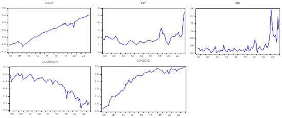
Figure 2.
Time plots of the variables (from 2006 to 2023).
We applied standard unit root tests to analyze the data-generating processes of the variables, specifically the Augmented Dickey–Fuller (ADF) [52], Phillips–Perron (PP) [53], and Kwiatkowski–Phillips–Schmidt–Shin (KPSS) [54] tests. The ADF and PP tests assume the presence of unit roots in the null hypothesis. Conversely, the KPSS test assumes stationarity (or trend stationarity) in the null hypothesis and tests it against the alternative hypothesis of non-stationarity. The results are reported in Table 5. The unit root tests in general point to unit roots in levels and stationarity in first differences. We also investigate whether non-stationarity in time series results from structural breaks rather than inherent stochastic trends [55]. The test results show that the order of integration in the variables remains unchanged even when structural breaks are considered.
Table 5.
Unit root tests (Δ denotes first difference operator).
4. Analysis and Results
4.1. Cointegration
To examine the presence of cointegration among the variables, we employed Johansen’s multivariate approach [56]. We first defined a vector autoregressive (VAR) model:
where , , p is the order (lag length) of the VAR, and are white noise residuals. Cointegration within this VAR model is modeled via associated vector error correction (VEC) representation:
where , is the loading matrix (the coefficient of the cointegrating vector in each error correction equation), and is matrix of cointegrating vectors. The rank r of the matrix represents the number of cointegrating vectors. If r = 0, then there is no cointegration among the variables, and a VAR analysis in the first differences would be appropriate. If r = 5 (the number of endogenous variables), then the variables are stationary and a VAR analysis in levels would be called for.
Before testing for cointegration, the deterministic terms, i.e., the coefficients of the intercept and the trend ( and or equivalently ) must be specified, since the critical values of the cointegration tests depend on these terms. We considered two cases:
- Restricted intercept with no time trend (Case 2): It assumes no linear trends in the data and a zero mean for the first-differenced series.
- Unrestricted intercept with no time trend (Case 3): It allows for linear trends in the data, and non-zero intercept in the cointegrating relations.
Economic theory suggests that first differences in interest rates, inflation, and real effective exchange rates should have zero unconditional means in the steady state, while the first differences of the log of real GDP and log of digital payments should have non-zero means. Thus, Case 2 appears more appropriate for the first three variables, while Case 3 is more appropriate for the latter two. We deferred the final model selection to the Johansen test results as described later.
To ensure a correctly specified system, we selected the lag order using the Schwarz Information Criterion (SIC), which favors more parsimonious models compared to the Akaike Information Criterion (AIC). This is particularly important given our relatively small sample size since AIC tends to overfit, i.e., it selects models with too many parameters. The SIC suggests a lag length of 2.
We then assessed the adequacy of the unrestricted VAR (2) model by conducting diagnostic tests on the residuals, including:
- LM tests for autocorrelation up to 1st, 4th, and 8th lags.
- The Doornik and Hansen multivariate test for normality.
- A White-type test for heteroskedasticity.
The diagnostic statistics on the system residuals, reported in Table 6, indicate that our VAR model with k = 2 performs reasonably well over the estimation sample, despite the presence of some non-normality in the residuals. This non-normality is primarily driven by excess skewness and kurtosis in the residuals of the interest rate and inflation equations, which in turn may be caused by high inflation and high interest rates in recent years in Turkey.
Table 6.
Diagnostic tests on the VAR model.
We applied the Johansen [56] integration tests procedure, which sequentially tests from the most to the least restrictive model, comparing the trace test statistic to its critical value at each stage and stopping when the null hypothesis is not rejected. The trace statistic is typically preferred to the maximal eigenvalue statistic since the latter is generally less robust to the presence of skewness and excess kurtosis in the errors [57]. Given that we have evidence of non-normality in the residuals of the VAR model, we relied on the trace statistics in our analysis.
The results for cointegration tests are presented in Table 7, from the most restrictive alternative (r = 0 and Model (i)) to the least restrictive alternative (r = n − 1 and Model (ii), where n is the number of endogenous variables). The first instance where the null hypothesis is not rejected is highlighted in bold. Accordingly, the procedure suggests one cointegration vector (r = 1) and that there are deterministic trends in the levels of the data but no trend in the cointegrating vector (Model (ii)).
Table 7.
Johansen cointegration test results.
Table 8 presents the estimation results for the cointegrating vector when normalized with respect to the GDP.
Table 8.
Estimation results for the single cointegrating vector.
The results imply that:
- A 1% increase in interest rates is associated with a 0.4% decrease in real GDP. This aligns with conventional monetary theory—in periods when interest rates are higher, economic activity may slow down due to a rise in borrowing costs. However, the insignificance of the coefficient suggests that interest rates may not be the primary driver of GDP growth (or vice versa) in the long term.
- A 1% increase in inflation is associated with a 3.1% decrease in real GDP. High inflation and low economic growth may coincide for several reasons. For example, low growth may lead to higher inflation through supply problems or inflation may reduce growth through lower purchasing power, increased uncertainty, and potential distortions in savings and investment behavior.
- A 1% increase in real effective exchange rates (appreciation of the domestic currency) is associated with a 0.8% increase in real GDP, i.e., a stronger domestic currency goes hand in hand with higher growth in Turkey. This result is not surprising since Turkey is a chronic current account deficit country, and the economy heavily relies on the inflow of foreign capital for investment and economic growth. When capital inflows intensify, economic growth accelerates together with stronger domestic currency.
- A 1% increase in the volume of digital payments is associated with a 0.2% increase in real GDP. This highlights the positive correlation between digitalization and economic growth.
We investigated the weak exogeneity of the endogenous variables by testing the exclusion of the cointegration vector from each of the five error-correction equations (one for each endogenous variables) [56,58]. Weak exogeneity refers to a situation where a variable is exogenous with respect to the parameters of interest in a model, but not necessarily with respect to the full system of equations. A weakly exogenous variable may still be influenced by other factors, but it does not affect the estimation of parameters in the cointegrating vector.
According to the test results reported in Table 9, weak exogeneity is rejected for real GDP (), inflation (), and digital payments (). This means that any long-run disequilibrium in the cointegrating relationship is corrected through adjustments in these variables. Weak exogeneity cannot be rejected for the other two endogenous variables (interest rates, , and exchange rates, ). Hence, interest rates and exchange rates are long-term forcing variables for real GDP, inflation, and digital payments, but not vice-versa. Note that this does not preclude short-run Granger causality. Real GDP, inflation, and digital payments may still affect interest rates or exchange rates in the short run. However, there is no feedback from the cointegrating vector into these two variables.
Table 9.
Weak exogeneity test on regressors.
4.2. Estimation of Vector Error Correction Model (VECM)
The existence of cointegration reveals a long-run relationship among the endogenous variables but does not point out the direction of causality. One way to address this issue is Granger causality tests. Pairwise tests (unconditional test) are more convenient but fail to control the impact of other variables. Multivariate tests (conditional test) enable the estimation of both “short-run” causality (through the coefficient of lagged first-differenced variables in the vector error-correction model) and the “long-run” causality (through the coefficient of the error-correction term), but the results may be misleading as it is not possible to determine which explanatory variable drives causality through the error correction term [59]. Nevertheless, both tests provide valuable insights into potential linkage among the variables. As a preliminary step, we applied Granger tests, first pairwise and then in a multivariate setting. The results are reported in Table 10. The evidence is mixed. In the pairwise tests, GDP Granger-causes interest rates and exchange rates, whereas in the multivariate setting, the direction of causality is reversed. In pairwise tests, digital payments and GDP do not Granger-cause each other, but the multivariate tests suggest a bidirectional relationship.
Table 10.
Granger causality tests on endogenous variables.
To better understand causal relationships, we estimated the dynamic model in first differences (the so-called short-term parameters) via a VECM and relied on impulse response analysis. Our system of equations consisted of three conditional models for the endogenous variables, (, , ) and two marginal models for the weakly exogenous variables (, ). While parameters of the endogenous variables can be estimated independently of the weakly exogenous variables, impulse response analysis requires specifying the processes that drive the weakly exogenous variables.
We used the following VECM:
Equation (4) corresponds to the conditional error correction models for the endogenous variables , whereas Equation (5) corresponds to the marginal error correction models for the weakly exogenous variables . Note that , where represents the error-correction term and equals to the cointegrating vector. The parameter of the cointegrating vector is restricted to zero in the marginal model by definition of weak exogeneity. The two models are correlated via .
A dynamic model must consider the country specific shocks and the global environment, such as global economic activity and global financial conditions, which are critical for a small, open economy like Turkey. For that reason, we included a set of exogenous variables, in our VECM, which are as follows:
- : Quarterly percentage change in the federal funds rate.
- : Quarterly change in the log of real GDP of the Euro area.
- and : Dummy variables capturing the impact of two non-economic shocks. One is the failed coup attempt in Turkey in July 2016 and the other is the Covid19 epidemic in March 2020. is equal to one in 2016Q3, minus one in 2016Q4, and zero otherwise. is equal to one in 2020Q2, minus one in 2020Q3, and zero otherwise.
We used the GDP of the Euro area as a proxy for global economic activity since Europe is Turkey’s major destination of exports. Likewise, our use of the federal funds rate stemmed from the fact that the financial conditions in the USA are the major driver of global funds destined for emerging markets [60,61]. We checked the order of integration in these variables via unit-root tests (ADF, PP, and KPSS) and confirmed that they are stationary in their first differences.
In addition to non-economic shocks, Turkey has also experienced a number of macroeconomic shocks, most notably the 2008 Global Financial Crisis, and the local 2018 exchange rate shock. We also created dummy variables for these macroeconomic shocks, but the estimated coefficients were insignificant in the model (most importantly in the GDP equation), suggesting that these shocks lead to adjustments within the system and do not cause any “unexplained” shock to the GDP.
The estimation results are reported in Table 11. The coefficient of the error correction term () illustrates how quickly the long-run relationships will be re-established if the system is hit by a shock. Its value in the GDP growth rate () equation is 0.041. The corresponding half-life of the adjustment is approximately 17 quarters, i.e., following a one-time deviation from the long-run equilibrium, it takes about 4 years for real GDP to adjust halfway to its equilibrium. This demonstrates a quite slow convergence to the long-run steady state, suggesting the presence of structural rigidities. Half-life is 10 quarters in the case of inflation () and only 2 quarters in the case of digital payments (). Hence, digital payments adjust to shocks significantly faster than GDP and inflation, indicating a high level of responsiveness in financial technology adoption.
Table 11.
Estimation of the VECM.
Analyzing each equation in the VECM separately, we observed that:
- Digital banking has a positive and significant coefficient, supporting the view that financial digitalization facilitates economic growth. A 1% increase in the quarterly growth of digital banking usage raises the quarterly growth rate of the GDP by 0.05 percentage points. The short-term impact of interest rates is significant but negative, reflecting the contractionary impact of monetary tightening. Exchange rate (appreciation of the domestic currency) has a significant and positive effect on economic growth as stronger currency cheapens imports, reduces costs for businesses and consumers, and lowers the external debt burden. Out of two exogenous factors, the change in federal funds rate is not significant, possibly due to the presence of exchange rates in the model that captures the influence of global financial conditions. The growth rate of the Euro area, on the other hand, has a significant and positive coefficient, showing the importance of global demand conditions. Finally, the dummy variable, , is significant and negative, reflecting the adverse effect of the failed coup attempt that is not captured by regular variables, whereas is negative but not significant, which suggests that its impact on GDP is already captured by other regressors. The model explains over 81% of the variation in .
- In the (quarterly change in the inflation rate) equation, the coefficients of most variables have expected signs, but only the growth rate, the change in exchange rates, and the change in the federal funds rate are statistically significant. The positive link between growth and inflation in Turkey reflects the boom-and-bust cycles experienced since 1980s. The negative effect of tightening in global financial conditions and the positive effect of currency depreciation on inflation are common themes in emerging market economies. The explanatory power of the model is modest: R2 is 0.520.
- In the (quarterly change in the growth rate of digital payments) equation, the coefficients of the error correction term and the growth rate are significant, reflecting the positive link between the growth rate and digital payments. The explanatory power of the model is also modest: R2 is 0.349.
- Plotting the recursive estimates and confidence intervals provides useful information on possible structural breaks. For that purpose, we dropped the dummy variables and and analyzed the recursive residuals, CUSUM and CUSUM-of-squares, of the equation. The corresponding figures are presented in Figure 3. A visual inspection on recursive residuals shows one structural break in 2016, which coincides with the failed coup attempt in July 2016 and justifies the use of the dummy variable in our analysis. The CUSUM line stays within the critical bounds. Hence, the null hypothesis of parameter stability cannot be rejected, indicating a stable model. Similarly, the CUSUM-of-squares plot suggests stable variance.
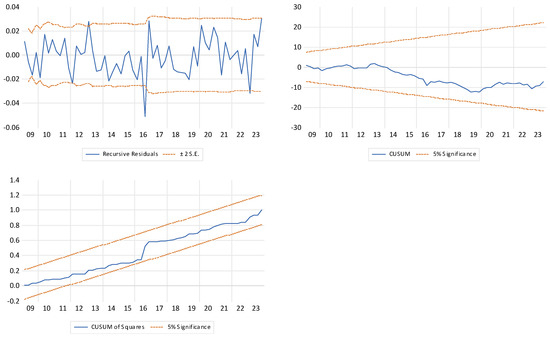 Figure 3. Stability analysis for the real GDP (logy) of Turkey (X-axis shows years). The first figure shows the recursive residuals over time, along with ±2 standard error bands. The CUSUM plot illustrates the cumulative sum of recursive residuals over time, along with the 5% significance bounds. The CUSUM-of-squares plot shows the cumulative sum of squared recursive residuals, along with the 5% significance bounds.
4.3. Generalized Impulse Response Functions and Variance Decomposition Analysis
Interpreting the estimated coefficients of a VAR or VECM model can be difficult due to the complex interdependence between variables. Notably, a shock to an endogenous variable not only directly affects that variable but is also transmitted to other endogenous variables through the dynamic (lag) structure of the VAR. The primary method of examining the properties of a dynamic system of equations is impulse response function (IRF) analysis, which traces the impact of a shock to a single variable on the current and future values of all the endogenous variables. However, in a VECM framework, shocks are typically correlated contemporaneously, unless the error covariance matrix is diagonal. In our case, the residual correlation matrix reveals significant contemporaneous correlations among the shocks, which makes it difficult to attribute forecast errors to a single equation:
Some off-diagonal elements are relatively sizable. For example, the correlation between the residuals of and is 0.36; that of and is 0.34; that of and is −0.34. If these contemporaneous correlations are not addressed and modeled adequately, the dynamic interactions among variables may be misinterpreted.
The conventional practice in the VAR literature is to impose some restrictions to identify the shocks, such as the Cholosky decomposition, long-run restrictions, etc. However, the imposed structure is mostly arbitrary. To avoid such subjectivity, we employed the generalized impulse response function (GIRF) approach proposed by Pesaran and Shin [62]. This method accounts for the correlation structure of the errors and offers a theoretically neutral way to derive impulse responses.
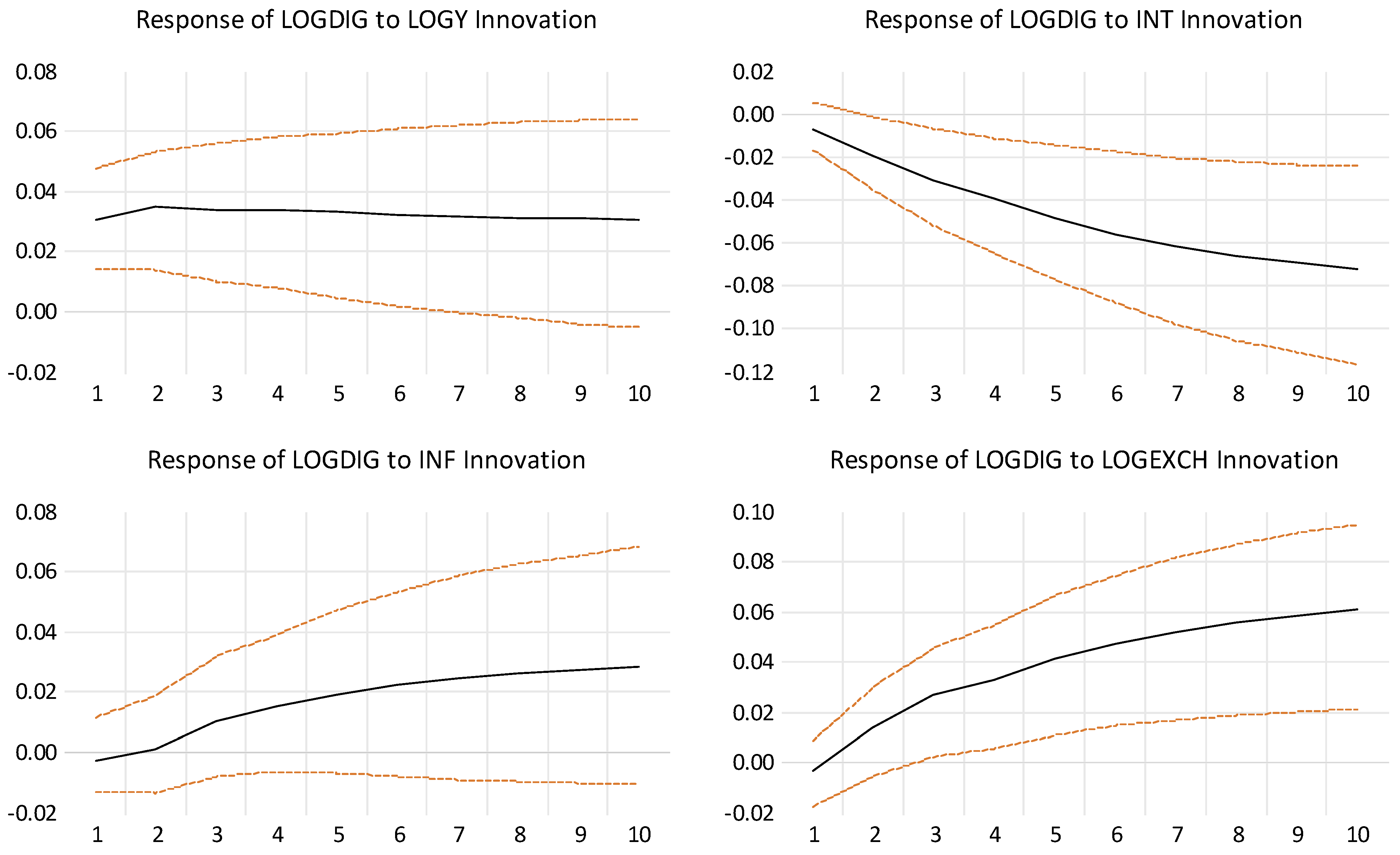
The generalized impulse responses, illustrated in Figure 4, reveal the following key patterns on the determinants of the real GDP in Turkey, :
- A one standard error rise in interest rates, , leads to a persistent downward revision in the growth rate of GDP, with the effect remaining statistically significant at the 95% confidence interval. The result confirms the conventional wisdom that higher borrowing costs dampen economic activity.
- A similar shock in inflation, , would also result in a permanent reduction in GDP growth. This highlights the role played by inflation as a major constraint on long-term growth, emphasizing the importance of maintaining price stability.
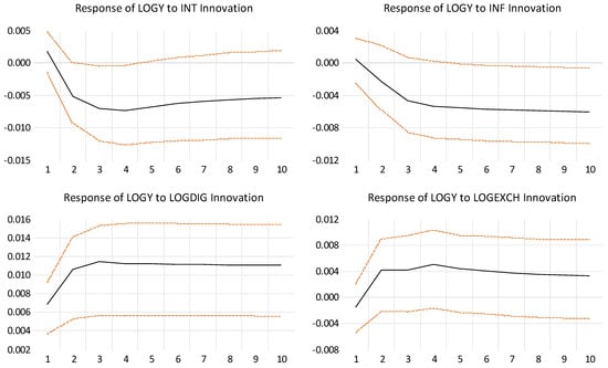
Figure 4.
Impulse response of logy (real GDP) to one standard deviation innovations in int (interest rates), inf (inflation), logexch (real exchange rate), and logdig (digital payment) with ±2 standard bands (dotted lines). The X-axis shows the number of quarters after the shock. The Y-axis shows the percentage change in the response variable. The responses are derived from the coefficient estimates of the VECM model in Table 11.
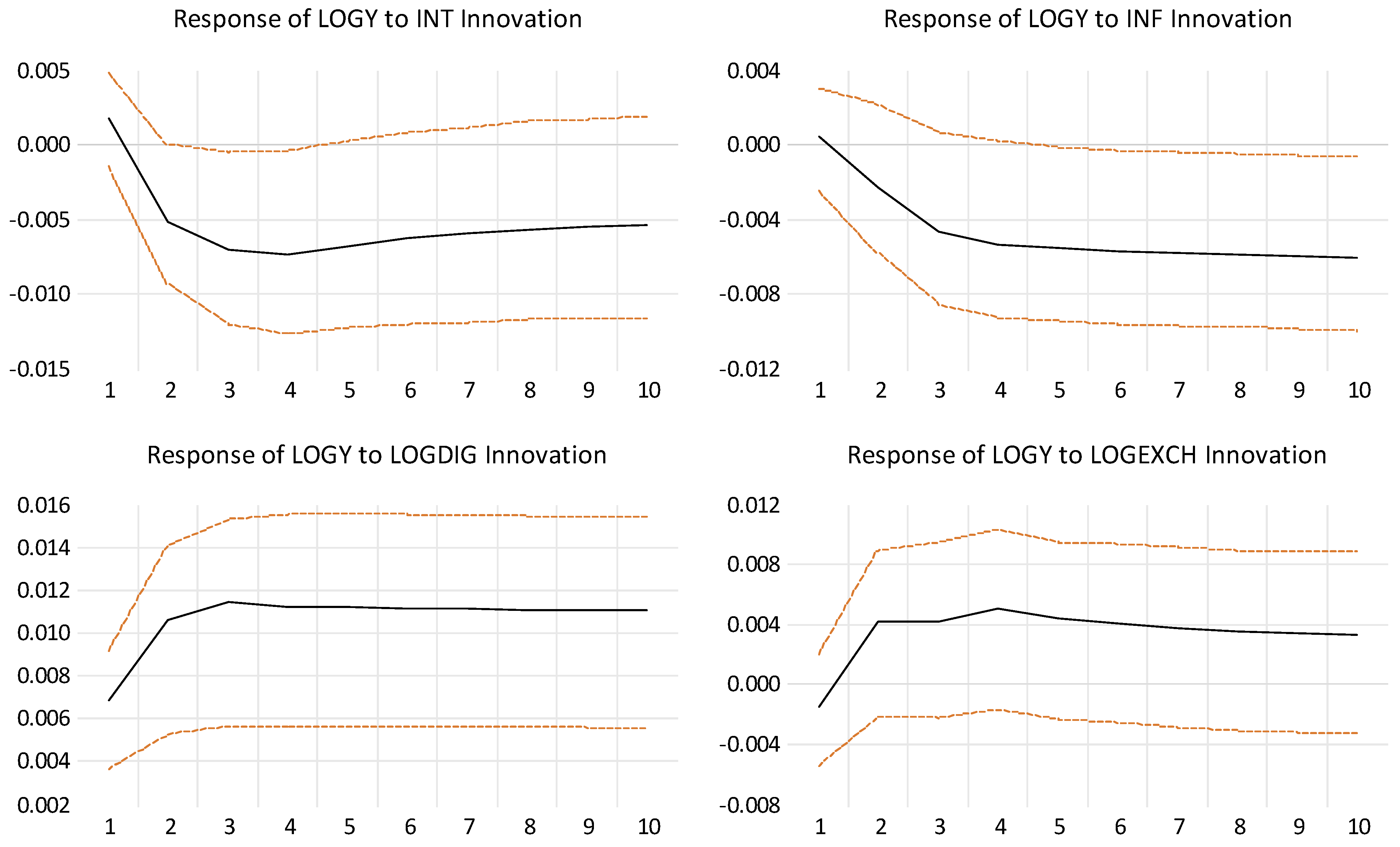
- An appreciation of the domestic currency (a rise in the real effective exchange rate, ) leads to a rise in the growth rate of GDP. This suggests that the domestic economy benefits from stronger currency, possibly through improved capital inflows or reduced import costs and foreign debt. However, this is not a permanent effect as the economy returns to its long-run equilibrium over time.
- Finally, a positive shock to the volume of digital payment, , leads to a permanent rise in the growth rate of GDP, which is significantly different than zero. This finding supports the argument that digitalization promoted economic activity.
We also analyzed the generalized impulse responses of the digital payment, , to understand its determinants. The results are presented in Figure 5. We found that:
- A positive shock to the real GDP, , leads to a permanent rise in the use of digital payments. Hence, digitalization is in harmony with the size of the economy. Larger economies naturally drive the shift to digital payments because of increased consumer demand, business needs, and technological advancements.
- A positive shock to the interest rates, , lowers the use of digital payments. The negative effect of financial conditions on digital payments is quite intuitive, since consumers and businesses reduce spending as financial conditions tighten.
- Interestingly, a positive shock in inflation, , raises the use of digital payments. As inflation rises, agents would be reluctant to hold cash, prompting people to adopt digital payments for speed and convenience.
- An appreciation of domestic currency (a rise in exchange rate, ) leads to a rise in the use of digital payments. A stronger currency boosts consumer confidence and purchasing power, encouraging more transactions.

Figure 5.
Impulse response of logdig (real volume of digital payments) to one standard deviation innovation in logy (real GDP), int (interest rates), inf (inflation), and logexch (real exchange rate) with ±2 standard bands (dotted lines). The X-axis shows the number of quarters after the shock. The Y-axis shows the percentage change in the response variable. The responses are derived from the coefficient estimates of the VECM model in Table 11.
Although IRF is valuable in understanding the causal relationship, it does not show the relative importance of each variable in explaining the dynamic behavior of the system. For that purpose, we employed a variance decomposition analysis (VCA), presented in Table 12, to quantify the proportion of the forecast error variance in each endogenous variable attributable to shocks in itself and other variables.
Table 12.
Variance decomposition analysis.
Initially, all endogenous variables are predominantly influenced by their own shock. Over time, the share of other variables increases, and, by the end of the 20th quarter, all four variables turn out to have almost the same share in explaining the forecast variance in the growth rate. This shows that interest rates, inflation, exchange rates, and digital payments are almost equally important in explaining growth dynamics of Turkey. Variation in inflation, on the other hand, is predominantly explained by shocks to itself and exchange rates, underscoring the importance of exchange rates in shaping inflation dynamics in small, open economies like Turkey. No variable, however, significantly explains the variation in exchange rates. Interest rates are mostly under the influence of inflation and exchange rates, which is also the common theme in small, open economies as well. Finally, the primary determinants of the variation in digital payment volume are exchange rates and interest rates. In comparison, GDP and inflation play a secondary role in explaining variations in digital payment usage. These findings underscore the critical impact of financial and monetary factors on digital transaction adoption, highlighting the need for stable exchange rate policies and interest rate management to support the expansion of digital financial services.
4.4. Transmission Channels
In our analysis, we examined the impact of digital payments on GDP while controlling a range of macroeconomic and financial variables. Although this approach offers valuable insights about the effect of digital payments on economic development, it does not explicitly address the mechanisms through which this relationship operates. Understanding these transmission channels is crucial, as it enables policymakers to design targeted interventions that maximize the developmental potential of digital finance.
In this section, we turn our attention to three key channels through which digital payments may plausibly affect GDP: household consumption, productivity, and financial intermediation. These channels are frequently highlighted in the literature as core pathways linking digital financial technologies to broader economic outcomes (e.g., [25,63,64]).
While a rigorous empirical identification of these channels is beyond the scope of this paper, we adopted a stepwise approach to explore their relevance using the same VAR framework employed in our analysis. Specifically, in each case, we replaced the dependent variable () with an alternative variable that proxies for one of the three hypothesized transmission channels. This approach allows us to assess whether digital payment usage is systematically associated with movements in these intermediary outcomes over time.
The first channel through which digital payments may stimulate economic activity is household consumption. To investigate this channel, we used data on total household consumption expenditure, in both aggregate terms and its subcomponents:
- Durables: Including items such as vehicles and household appliances.
- Semi-durables: Items with a medium lifespan, such as clothing and electronics.
- Non-durables: Consumption goods such as food and fuel.
- Services: Including education, healthcare, transportation, and recreation, etc.
This breakdown allowed us to assess whether digital payment usage disproportionately affects specific types of consumption, which may in turn reflect differences in liquidity constraints or transaction costs. We used the seasonally adjusted data obtained from TURKSTAT on a quarterly basis.
The second channel through which digital payments may enhance economic performance is by improving productivity. As a proxy for (labor) productivity, we constructed three separate measures:
- Aggregate productivity.
- Sectoral productivity for industry.
- Sectoral productivity for services.
Each productivity measure was calculated as total value added divided by total hours worked, with data sourced from TURKSTAT’s labor and national accounts statistics.
The third channel is related to the access and efficiency of financial services. To capture this channel, we used two measures:
- Value added in the financial sector.
- Credit to GDP ratio.
The seasonally adjusted quarterly data for value added in the financial sector was obtained from TURKSTAT, while the credit to GDP ratio was calculated using total banking credit data reported by the Central Bank of Turkey.
The results are reported in three sections in Table 13.
Table 13.
(a) Transmission mechanism—consumption: estimates of the cointegrating vector. (b) Transmission mechanism—productivity: estimates of the cointegrating vector. (c) Transmission mechanism—financial services: estimates of the cointegrating vector.
We begin with the consumption channel in Part A of Table 13. The coefficient of the digital payments (logdig) in the cointegrating vector is consistently positive and statistically significant across all consumption measures. The results suggest that digital payments facilitate smoother and potentially more frequent transactions, thereby stimulating consumption. We also found considerable heterogeneity in the magnitude of this effect across consumption categories. The coefficient is higher for durable goods and lower for nondurable goods. One plausible explanation is that consumers are more likely to engage in digital transactions when making significant financial commitments, possibly due to the added convenience, security, and transparency associated with electronic payments for larger amounts. When the transaction value is low and/or more frequent, the perceived benefits of digital payments may be less pronounced. For everyday low-cost items, consumers might still prefer using cash.
In Part B of Table 13, we examined the link between digital payments and productivity. Although the coefficient for digital payments remains positive across all three productivity measures (aggregate, industrial, and services), it fails to reach statistical significance. This suggests that there is no strong or conclusive evidence supporting the hypothesis that digital payments enhance productivity at the macroeconomic level. A possible explanation is that the productivity measures employed may be too broad or rudimentary to capture the nuanced and potentially sector-specific effects of digital financial technologies.
Lastly, Part C of Table 13 investigates the role of financial intermediation as a potential transmission channel. We employed two indicators: (1) the value added in the financial sector and (2) the size of bank credit relative to the overall economy. In both cases, the coefficient for digital payments is statistically significant. These findings suggest that the widespread adoption of digital payment methods may be contributing to the deepening of financial markets by facilitating smoother and more efficient transactions, thus potentially increasing the volume of financial activity. Moreover, digital payments may provide greater access to financial services, especially in previously underserved or unbanked populations. This could lead to an expansion in the volume of financial transactions, thus boosting the overall contribution of the financial sector to economic output.
4.5. Robustness
In this section, we studied the robustness of the results to alternative estimation techniques for cointegration and alternative measures for digital payments. We also considered whether common factors, such as technological advances in digital technology that have the potential to impact both digital banking and economic growth, may bias the estimation results. Lastly, we investigated the presence of nonlinearities and threshold effects.
Our preferred method for estimating cointegration was VAR, since it addresses the endogeneity of all variables in question capturing dynamic interdependencies without imposing structural restrictions. There are several single equation methods, such as ARDL with the bounds testing approach, dynamic least squares (DOLS), or fully modified least squares (FMOLS), that assume one variable to be endogenous and others to be (weakly) exogenous. Single estimation methods are more efficient due to there being fewer parameters to be estimated and are typically preferred when one variable is the primary focus of the study. ARDL, in particular, can be applied to a mix of I(0) and I(1) variables, making it a more flexible approach. Single estimation methods, however, would yield biased estimates if structural restrictions (i.e., weak exogeneity of the other variables) were not valid.
To understand the sensitivity of our results to estimation methods, we estimated the cointegrating vector by ARDL, DOLS, and FMOLS. The results are reported in Table 14. The first column shows the estimates of our preferred method, the Johansen’s approach. The estimates based on ARDL, DOLS, and FMOLS are in the second, third, and fourth columns, respectively. Interest rates, which were insignificant in the Johansen’s method, turn out to be significant in DOLS and FMOLS, whereas inflation loses its significance. Digital payments, on the other hand, are significant and positive in all four models. Overall, we conclude that the cointegrating relation between economic growth and digital payment is robust to alternative estimation methods.
Table 14.
Estimates of the cointegrating vector using alternative estimation methods.
Digital transactions can be measured in different ways. While digital payments might arguably be the most accurate indicator of digital transactions, we explored the robustness of our results to alternative measures. These measures were:
- : volume of money transfers over mobile (smart phone) banking.
- : volume of money transfers over internet banking.
- : volume of credit card transactions over internet banking.
All variables were seasonally adjusted and in real log terms. The use of digital banking for money transfers may be an unreliable measure of digital transactions, as they often involve personal, non-commercial transactions and exclude other digital methods like mobile wallets, QR codes, or app-based payments. Credit card transactions may not be a good measure either, since they are just substitute in-person card transactions.
To apply Johansen’s method, we first constructed the appropriate VAR model for each alternative measure. The lag length was specified with SIC provided that the model satisfies diagnostic tests, in particular the absence of serial correlation. Next, we re-estimated the cointegrating vector expressed in Table 8 using these alternative measures for . The results are reported in Table 15.
Table 15.
Estimates of the cointegrating vector using alternative measures for logdig.
For comparison, we present the results of our preferred measure in the first column. The coefficients of all alternative measures are positive and statistically significant at 1%, possibly due to high correlation across alternative methods of digital banking. However, the magnitude of the coefficient is low with respect to the coefficient of our baseline model when the alternative measure is the volume of online transfers via mobile phone or internet banking. The coefficient is much higher when the alternative measure is the volume credit card transactions over the internet. Regardless of the magnitude of the estimated coefficients, the statistical significance of the results suggests that the link between digital transactions and GDP is robust to alternative measures.
Although several macroeconomic and financial variables were included as control variables in our model, there may exist some unobserved common factors that simultaneously influence both digital banking and GDP, potentially leading to biased estimates if omitted. One such factor is technological advances, which may independently contribute to economic growth, beyond its indirect effects through digital payment. To account for this concern, we incorporated two proxy measures of technological progress:
- : the number of internet users per 100 people.
- : the number of mobile cellular subscriptions per 100 people.
Both variables were obtained from TURKSTAT and were incorporated sequentially into the VAR model to assess their impact on the cointegrating relationship. The estimation results are presented in Table 16.
Table 16.
Estimates of the cointegrating vector controlling common factors (technological progress).
In both cases, the Johansen cointegration test indicates the presence of a single cointegrating vector. When internet usage is introduced into the model, the coefficient associated with digital payments declines in magnitude but remains statistically significant. Concurrently, the coefficient on internet usage is both positive and statistically significant, suggesting that part of the explanatory power attributed to digital payments may, in fact, be captured by internet usage. In contrast, when the second measure of technological advances, mobile cellular subscriptions, is added to the model, its coefficient is statistically insignificant, whereas the coefficient on digital payments remains significant and slightly higher in magnitude.
Another robustness issue pertains to potential nonlinearities and threshold effects in the relationship under investigation. While the baseline model assumes a linear cointegrating relationship among variables, it is plausible that this link may, in fact, be nonlinear implying that distinct cointegrating vectors may characterize different regimes. For instance, the positive impact of digital payments on growth may only materialize under certain macroeconomic conditions such as positive economic growth, low inflation or interest rates, or currency appreciation.
To address this issue, we re-estimated the cointegrating vector using the threshold cointegration methodology proposed by Balke and Fomby (1997) for univariate models and extended by Hansen and Seo (2002) for multivariate models. This approach allows for the identification of regime-dependent dynamics by employing an indicator function that determines regime transitions based on threshold behavior. For example, a two-regime VECM with a single cointegrating vector can be expressed in the following form:
where is the vector of endogenous variables, is the coefficient matrix with corresponding loading matrix and cointegrating matrix at regime I, I(.) is the indicator function, is the threshold variable that determines the regime, and is the threshold value. The threshold variable can be the error-correction term or any stationary transformation of the predetermined variables.
As threshold variables, we considered both quarterly and one-year lagged differences of the endogenous variables. Since the threshold values were not known, the model was estimated for all possible values within the sample that the threshold indicator may take. To mitigate the risk of overfitting, the set of admissible threshold values was restricted such that each regime contained at least 15% of the sample, in addition to the number of estimated coefficients. The optimal threshold and associated coefficient matrices were those that maximize the log-likelihood function, under the assumption of independently and identically distributed Gaussian errors. To test the null hypothesis of linear cointegration against the alternative of threshold cointegration, we employed Lagrange multiplier statistics. p-values were computed using a parametric bootstrap procedure with 5000 replications.
The linear VAR model was rejected with p-value = 0.039 in favor of the threshold VAR model in only one instance: when the one quarter lagged change in interest rates was employed as the stationary threshold variable with a threshold value of 0.002. The corresponding estimation results from the TVAR model are presented in Table 17, with the baseline linear VAR estimates reported in the first column for comparative purposes.
Table 17.
Estimates of the cointegrating vector: comparison of VAR and threshold VAR models.
The TVAR model delineates two distinct regimes based on prevailing monetary conditions. Specifically, when the quarterly change in interest rates is below 0.2%—interpreted as a period of “monetary loosening”—the long-run impact of digital payments on GDP is estimated at 0.266. In contrast, during periods of “monetary tightening,” defined by a quarterly interest rate change exceeding 0.2%, the long-run effect is comparatively lower at 0.158. For reference, the linear VAR model—which does not account for regime shifts—yields a single long-run estimate of 0.227 for the cointegrating vector associated with digital payments. The results suggest that, even in the presence of threshold effects, the positive link between digital payments and growth persists.
5. Conclusions
This study investigates the dynamic relationship between digital payments and sustainable economic growth in Turkey, utilizing quarterly data from 2006 to 2023 and a VAR framework. A positive and statistically significant cointegrating relationship is estimated between GDP and digital payments, suggesting that financial digitalization and macroeconomic growth are closely linked over time. Granger causality tests and impulse response analysis indicate a bidirectional association between digital payments and GDP growth, suggesting that policies fostering both economic resilience and digital adoption may generate mutually reinforcing benefits.
We also explore key transmission mechanisms through which digital payments may affect economic activity. We found that digital payments are associated with increased consumer expenditure, particularly for durable goods, reflecting the role of convenience and security in encouraging higher value transactions. While the effect on labor productivity is positive, it does not reach statistical significance, indicating that productivity gains may depend on broader structural or technological factors. Furthermore, digital payments significantly enhance financial intermediation by increasing financial sector value added and expanding bank credit, highlighting their role in deepening financial markets and improving financial access.
The analysis further identifies the determinants of digital transactions. GDP, inflation, and real exchange rates are positively associated with digital payment usage, while higher interest rates appear to deter adoption. The variance decomposition analysis indicates that exchange rates and interest rates contribute to the most to variations in digital payments, with GDP and inflation playing a secondary role.
A key contribution of this paper lies in its context-specific approach. By focusing on Turkey—an economy characterized by persistent inflation, structural reforms, and a rapidly evolving digital banking ecosystem—the findings offer a compelling case for understanding financial digitalization in emerging markets. The macro-level VAR/VECM framework demonstrates how digital payments can serve as both an outcome and a driver of economic growth, particularly during periods of economic instability. This research underscores the importance of tailoring digital payment strategies to regional and macroeconomic realities.
Despite its contributions, this study has several limitations. First, the analysis was conducted at the aggregate macroeconomic level, which may obscure heterogeneity across regions, income groups, or sectors. Furthermore, unobserved factors such as informal economic activity, trust in financial institutions, or user behavior dynamics were not directly captured. Future research could address these gaps by incorporating micro-level data, or exploring mediating factors such as financial literacy, institutional trust, and technological readiness. Additionally, integrating datasets on informality, financial inclusion, and digital literacy could enrich the analysis and provide a more comprehensive understanding of how digital payments influence economic growth. Finally, a detailed investigation of transmission channels would enhance our understanding of the nuanced role of digital finance in emerging economies.
6. Policy Implications
Given Turkey’s unique macroeconomic environment characterized by persistent inflation, currency volatility, and a large informal economy, the results of this study offer several important policy recommendations. First, strengthening digital infrastructure in rural and underbanked areas is crucial to ensure economic growth. Initiatives such as subsidized mobile internet, QR-code-based payment systems, and mobile wallet integration can promote broader adoption. Second, government-led programs incentivizing SMEs to transition to digital payments—through tax rebates, access to micro-financing, and digital certification—could improve financial transparency and support formalization. Third, enhancing digital financial literacy among the population, especially youth and low-income groups, will help build user trust and boost adoption. Lastly, to sustain trust in digital financial systems, it is essential to implement strong cybersecurity measures, ensure the reliability of payment platforms, and build a sound regulatory environment that balances innovation with consumer protection. Establishing a secure and transparent digital payments ecosystem is essential for sustaining confidence in financial technology and preventing risks associated with cyber threats and fraud.
Author Contributions
Conceptualization, E.K. and T.G.; methodology, T.G.; software, T.G.; validation, T.G.; formal analysis, T.G.; resources, E.K. and T.G.; data curation, T.G.; writing—original draft preparation, E.K.; writing—review and editing, T.G.; visualization, T.G.; supervision, T.G. All authors have read and agreed to the published version of the manuscript.
Funding
This research received no external funding.
Institutional Review Board Statement
Not applicable.
Data Availability Statement
Conflicts of Interest
The authors declare no conflicts of interest.
Abbreviations
The following abbreviations are used in this manuscript:
| ADF | Augmented Dickey–Fuller |
| AIC | Akaike information criterion |
| ARDL | Autoregressive distributive lag |
| DOLS | Dynamic least squares |
| e-money | Electronic money |
| ECT | Error-correction term |
| FMOLS | Fully modified least squares |
| GDP | Gross domestic product |
| GIRF | Generalized impulse response function |
| IRF | Impulse response function |
| KPSS | Kwiatkowski–Phillips–Schmidt–Shin |
| OIC | Organization of Islamic Cooperation |
| PP | Phillips–Perron |
| SIC | Schwarz information criterion |
| TURKSTAT | Turkish Statistical Institute |
| VAR | Vector autoregressive |
| VCA | Variance decomposition analysis |
| VECM | Vector error correction model |
References
- Cull, R.J.; Foster, V.; Jolliffe, D.M.; Lederman, D.; Mare, D.S.; Veerappan, M. Digital Payments and the COVID-19 Shock: The Role of Preexisting Conditions in Banking, Infrastructure, Human Capabilities, and Digital Regulation; World Bank Group: Washington, DC, USA, 2023; Available online: http://documents.worldbank.org/curated/en/099454311132327828/IDU08c76166f0dda20435909e82051f6aa962419 (accessed on 12 December 2024).
- Anwar, C.J.; Ayunda, V.T.; Suhendra, I.; Ginanjar, R.A.F.; Kholishoh, L.N. Estimating the effects of electronic money on the income velocity of money in Indonesia. Int. J. Innov. Res. Sci. Stud. 2024, 7, 390–397. [Google Scholar] [CrossRef]
- Liu, X.; Liu, Q. Study on the Influence of Internet Payment on the Velocity of Money Circulation in China. In Business Intelligence and Information Technology; Hassanien, A.E., Xu, Y., Zhao, Z., Mohammed, S., Fan, Z., Eds.; Lecture Notes on Data Engineering and Communications Technologies; Springer International Publishing: Cham, Switzerland, 2022; Volume 107, pp. 577–593. [Google Scholar] [CrossRef]
- Putra, H.S.; Huljannah, M.; Putri, M. Analysis of the Demand for Money and the Velocity of Money in the Digital Economy Era: A Case Study in Indonesia. Jurnal REP 2021, 6, 110–125. [Google Scholar] [CrossRef]
- Ujunwa, A.; Onah, E.; Ujunwa, A.I.; Okoyeuzu, C.R.; Kalu, E.U. Financial innovation and the stability of money demand in Nigeria. Afr. Dev. Rev. 2022, 34, 215–231. [Google Scholar] [CrossRef]
- Prabheesh, K.P.; Affandi, Y.; Gunadi, I.; Kumar, S. Impact of Public Debt, Cashless Transactions on Inflation in Emerging Market Economies: Evidence from the COVID-19 Period. Emerg. Mark. Financ. Trade 2024, 60, 557–575. [Google Scholar] [CrossRef]
- Aguilar, A.; Frost, J.; Guerra, R.; Kamin, S.; Tombini, A. Digital Payments, Informality and Economic Growth. Bank for International Settlements 2. 2024. Available online: https://www.bis.org/publ/work1196.pdf (accessed on 30 January 2025).
- Marmora, P.; Mason, B.J. Does the shadow economy mitigate the effect of cashless payment technology on currency demand? dynamic panel evidence. Appl. Econ. 2021, 53, 703–718. [Google Scholar] [CrossRef]
- Setor, T.K.; Senyo, P.K.; Addo, A. Do digital payment transactions reduce corruption? Evidence from developing countries. Telemat. Inform. 2021, 60, 101577. [Google Scholar] [CrossRef]
- Kasri, R.A.; Indrastomo, B.S.; Hendranastiti, N.D.; Prasetyo, M.B. Digital payment and banking stability in emerging economy with dual banking system. Heliyon 2022, 8, e11198. [Google Scholar] [CrossRef]
- Li, J.; Wu, Y.; Xiao, J.J. The impact of digital finance on household consumption: Evidence from China. Econ. Model. 2020, 86, 317–326. [Google Scholar] [CrossRef]
- Zhou, R. Sustainable Economic Development, Digital Payment, and Consumer Demand: Evidence from China. Int. J. Environ. Res. Public Health 2022, 19, 8819. [Google Scholar] [CrossRef]
- Birigozzi, A.; De Silva, C.; Luitel, P. Digital payments and GDP growth: A behavioural quantitative analysis. Res. Int. Bus. Financ. 2025, 75, 102768. [Google Scholar] [CrossRef]
- Hasan, I.; De Renzis, T.; Schmiedel, H. Retail Payments and Economic Growth. Bank of Finland, Research Paper 19. 2012. Available online: https://ideas.repec.org//p/zbw/bofrdp/rdp2012_019.html (accessed on 1 February 2025).
- Patra, B.; Sethi, N. Does digital payment induce economic growth in emerging economies? The mediating role of institutional quality, consumption expenditure, and bank credit. Inf. Technol. Dev. 2024, 30, 57–75. [Google Scholar] [CrossRef]
- Tee, H.-H.; Ong, H.-B. Cashless payment and economic growth. Financ. Innov. 2016, 2, 4. [Google Scholar] [CrossRef]
- Wong, T.-L.; Lau, W.-Y.; Yip, T.-M. Cashless Payments and Economic Growth: Evidence from Selected OECD Countries. J. Cent. Bank. Theory Pract. 2020, 9, 189–213. [Google Scholar] [CrossRef]
- Zhang, Y.; Zhang, G.; Liu, L.; De Renzis, T.; Schmiedel, H. Retail payments and the real economy. J. Financ. Stab. 2019, 44, 100690. [Google Scholar] [CrossRef]
- PwC. Digital Banking Overview and Potential in Turkey. 2021. Available online: https://www.strategyand.pwc.com/tr/digital-banking-overview-and-potential-in-turkey (accessed on 12 February 2025).
- Etï, H.S. Effect of the COVID-19 Pandemic on Electronic Payment Systems in Turkey. Sos. Bilim. Metinleri 2022, 2022, 142–165. [Google Scholar] [CrossRef]
- Kahveci, E.; Avunduk, Z.B.; Daim, T.; Zaim, S. The role of flexibility, digitalization, and crisis response strategy for SMEs: Case of COVID-19. J. Small Bus. Manag. 2024, 63, 1198–1235. [Google Scholar] [CrossRef]
- Yadav, V.; Das, A. Digital payments in India—How demonetization and COVID-19 shaped adoption? Econ. Lett. 2025, 246, 112074. [Google Scholar] [CrossRef]
- Bai, B.; Um, K.-H.; Lee, H. The strategic role of firm agility in the relationship between IT capability and firm performance under the COVID-19 outbreak. J. Bus. Ind. Mark. 2023, 38, 1041–1054. [Google Scholar] [CrossRef]
- Humphrey, D.; Willesson, M.; Bergendahl, G.; Lindblom, T. Benefits from a Changing Payment Technology in European Banking. J. Bank. Financ. 2006, 30, 1631–1652. [Google Scholar] [CrossRef]
- Demirguc-Kunt, A.; Klapper, L.; Singer, D.; Ansar, S.; Hess, J. The Global Findex Database 2017: Measuring Financial Inclusion and the Fintech Revolution; World Bank Publications: Washington, DC, USA, 2018. [Google Scholar]
- Zins, A.; Weill, L. The determinants of financial inclusion in Africa. Rev. Dev. Financ. 2016, 6, 46–57. [Google Scholar] [CrossRef]
- Chen, H.; Liu, Y.; Wang, Z. Can Industrial Digitalization Boost a Consumption-Driven Economy? An Empirical Study Based on Provincial Data in China. J. Theor. Appl. Electron. Commer. Res. 2024, 19, 2377–2399. [Google Scholar] [CrossRef]
- Demirgüç-Kunt, A.; Klapper, L. Measuring Financial Inclusion: Explaining Variation in Use of Financial Services across and within Countries. Econ. Act. 2013, 2013, 279–340. [Google Scholar] [CrossRef]
- Ozili, P.K. Impact of digital finance on financial inclusion and stability. Borsa Istanb. Rev. 2018, 18, 329–340. [Google Scholar] [CrossRef]
- Romer, P.M. Endogenous Technological Change. J. Political Econ. 1990, 98, 71–102. [Google Scholar] [CrossRef]
- Beck, T.; Pamuk, H.; Ramrattan, R.; Uras, B.R. Payment instruments, finance and development. J. Dev. Econ. 2018, 133, 162–186. [Google Scholar] [CrossRef]
- Szabó, I.; Ternai, K.; Prosser, A.; Kovács, T. The impact of digitalization on SMEs GDP contribution. Procedia Comput. Sci. 2024, 239, 1807–1814. [Google Scholar] [CrossRef]
- Daud, S.; Mohd, N.; Ahmad, A.H. Financial inclusion, economic growth and the role of digital technology. Financ. Res. Lett. 2023, 53, 103602. [Google Scholar] [CrossRef]
- Kim, D.-W.; Yu, J.-S.; Hassan, M.K. Financial inclusion and economic growth in OIC countries. Res. Int. Bus. Financ. 2018, 43, 1–14. [Google Scholar] [CrossRef]
- Lo Prete, A. Digital and Financial Literacy as Determinants of Digital Payments and Personal Finance. Econ. Lett. 2022, 213, 110378. [Google Scholar] [CrossRef]
- Fernández-Portillo, A.; Almodóvar-González, M.; Hernández-Mogollón, R. Impact of ICT development on economic growth. A study of OECD European union countries. Technol. Soc. 2020, 63, 101420. [Google Scholar] [CrossRef]
- Prabheesh, K.; Rahman, R.E. Monetary Policy Transmission and Credit Cards: Evidence from Indonesia. Bull. Monet. Econ. Bank. 2019, 22, 137–162. [Google Scholar] [CrossRef]
- Tran, L.; Wang, W. Cashless Payments Impact to Economic Growth: Evidence in G20 Countries and Vietnam—Vietnamese Government with a Policy to Support Cashless Payments. Am. J. Ind. Bus. Manag. 2023, 13, 247–269. [Google Scholar] [CrossRef]
- Ravikumar, T.; Suresha, B.; Sriram, M.; Rajesh, R. Impact of Digital Payments on Economic Growth: Evidence from India. Int. J. Innov. Technol. Explor. Eng. 2019, 8, 553–557. [Google Scholar] [CrossRef]
- Reddy, K.S.; Kumarasamy, D. Is There Any Nexus between Electronic Based Payments in Banking and Inflation? Evidence from India. Int. J. Econ. Financ. 2015, 7, 85–95. [Google Scholar] [CrossRef]
- Mamudu, Z.U.; Gayovwi, G.O. Cashless Policy and Its Impact on The Nigerian Economy. Int. J. Educ. Res. 2019, 7, 111–132. [Google Scholar]
- Azeez, N.P.A.; Imdadul Haque, M.; Akhtar, S.M.J. Digital Payment and Economic Growth: Evidence from India. Appl. Econ. Q. 2022, 68, 79–93. [Google Scholar] [CrossRef]
- Givelyn, I.; Rohima, S.; Mardalena, M.; Widyanata, F. The Impact of Cashless Payment on Indonesian Economy: Before and During COVID-19 Pandemic. J. Ekon. Pembang. 2022, 20, 89–104. [Google Scholar] [CrossRef]
- Okoh, D.; Olopade, B.C.; Eseyin, O.S. Digital Payment And Economic Growth: Evidence From Nigeria. Int. J. Manag. Soc. Sci. Peace Confl. Stud. 2023, 6, 225–238. [Google Scholar]
- Bulut, E.; Çizgici Akyüz, G. Türkiye’de Dijital Bankacilik ve Ekonomik Büyüme İlişkisi. Marmara Üniversitesi İktisadi İdari Bilim. Derg. 2020, 42, 223–246. [Google Scholar] [CrossRef]
- Flores Segovia, M.A.; Torre Cepeda, L.E. Financial development and economic growth: New evidence from Mexican States. Reg. Sci. Policy Pract. 2024, 16, 100028. [Google Scholar] [CrossRef]
- Kahveci, E. Digital Transformation in SMEs: Enablers, Interconnections, and a Framework for Sustainable Competitive Advantage. Adm. Sci. 2025, 15, 107. [Google Scholar] [CrossRef]
- Kahveci, E. Digitalization, and Digital Transformation in MSMEs in Turkey. Int. J. Small Medium Enterp. Bus. Sustain. 2023, 8, 2. [Google Scholar]
- Sayar Özkan, G.; Çelik, H. Bilgi İletişim Teknolojileri İle Ekonomik Büyüme Arasindaki İlişki: Türkiye İçin Bir Uygulama. Uluslararası Ticaret Ekon. Araştırmaları Derg. 2018, 2, 1–15. [Google Scholar] [CrossRef]
- Bozkurt, V. Pandemi Döneminde Çalışma: Ekonomik Kaygılar, Dijitalleşme ve Verimlilik. In COVID-19 Pandemisinin Ekonomik, Toplumsal ve Siyasal Etkileri; Istanbul University Press: Istanbul, Turkey, 2020; pp. 115–136. [Google Scholar] [CrossRef]
- TURKSTAT. Survey on Information and Communication Technology (ICT) Usage in Households and by Individuals; Turkish Statistical Institute: Ankara, Turkey, 2022. Available online: https://data.tuik.gov.tr/Bulten/Index?p=Survey-on-Information-and-Communication-Technology-(ICT)-Usage-in-Households-and-by-Individuals-2022-45587 (accessed on 17 April 2025).
- Dickey, D.A.; Fuller, W.A. Distribution of the Estimators for Autoregressive Time Series With a Unit Root. J. Am. Stat. Assoc. 1979, 74, 427. [Google Scholar] [CrossRef]
- Phillips, P.C.B.; Perron, P. Testing for a unit root in time series regression. Biometrika 1988, 75, 335–346. [Google Scholar] [CrossRef]
- Kwiatkowski, D.; Phillips, P.C.B.; Schmidt, P.; Shin, Y. Testing the null hypothesis of stationarity against the alternative of a unit root. J. Econom. 1992, 54, 159–178. [Google Scholar] [CrossRef]
- Zivot, E.; Andrews, D.W.K. Further Evidence on the Great Crash, the Oil-Price Shock, and the Unit-Root Hypothesis. J. Bus. Econ. Stat. 1992, 10, 251–270. [Google Scholar] [CrossRef]
- Johansen, S. Estimation and Hypothesis Testing of Cointegration Vectors in Gaussian Vector Autoregressive Models. Econometrica 1991, 59, 1551. [Google Scholar] [CrossRef]
- Cheung, Y.; Lai, K.S. Finite-Sample Sizes Of Johansen’s Likelihood Ratio Tests For Cointegration. Oxf. Bull. Econ. Stat. 1993, 55, 313–328. [Google Scholar] [CrossRef]
- Harbo, I.; Johansen, S.; Nielsen, B.; Rahbek, A. Asymptotic Inference on Cointegrating Rank in Partial Systems. J. Bus. Econ. Stat. 1998, 16, 388–399. [Google Scholar] [CrossRef]
- Lütkepohl, H. Vector autoregressive models. In Handbook of Research Methods and Applications in Empirical Macroeconomics; Hashimzade, N., Thornton, M.A., Eds.; Edward Elgar Publishing: Melbourne, VIC, Canada, 2013. [Google Scholar] [CrossRef]
- Kahveci, E.; Odabaş, A. Central Banks’ Communication Strategy and Content Analysis of Monetary Policy Statements: The Case of Fed, ECB and CBRT. Procedia Soc. Behav. Sci. 2016, 235, 618–629. [Google Scholar] [CrossRef]
- Kahveci, E. Monetary Policy Strategies after The Global Financial Crisis: Comparison of Developed and Developing Country Experiences. In Economic Crises: A Review and Directions for Research; Economic Issues, Problems and Perspectives; Nova Science Publishers: New York, NY, USA, 2022; pp. 169–204. [Google Scholar] [CrossRef]
- Pesaran, H.H.; Shin, Y. Generalized impulse response analysis in linear multivariate models. Econ. Lett. 1998, 58, 17–29. [Google Scholar] [CrossRef]
- BIS. Annual Economic Report 2021. Available online: https://www.bis.org/publ/arpdf/ar2021e.htm (accessed on 28 April 2025).
- Suri, T.; Jack, W. The long-run poverty and gender impacts of mobile money. Science 2016, 354, 1288–1292. [Google Scholar] [CrossRef]
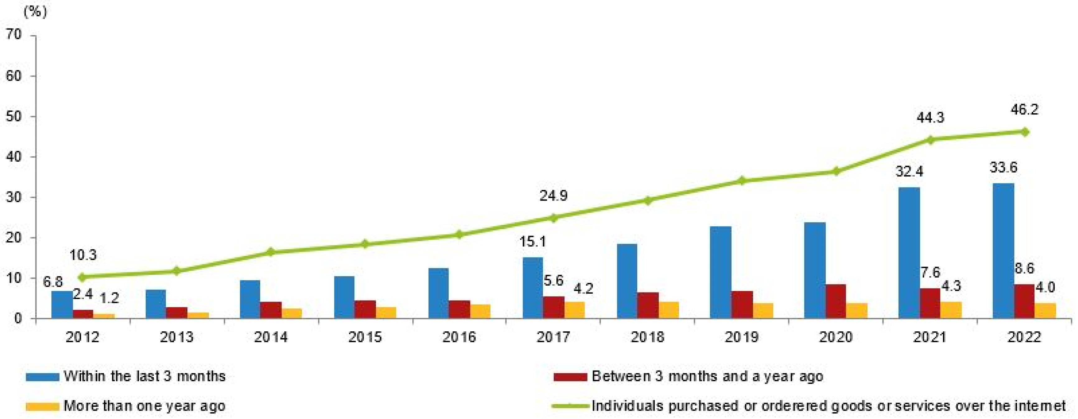
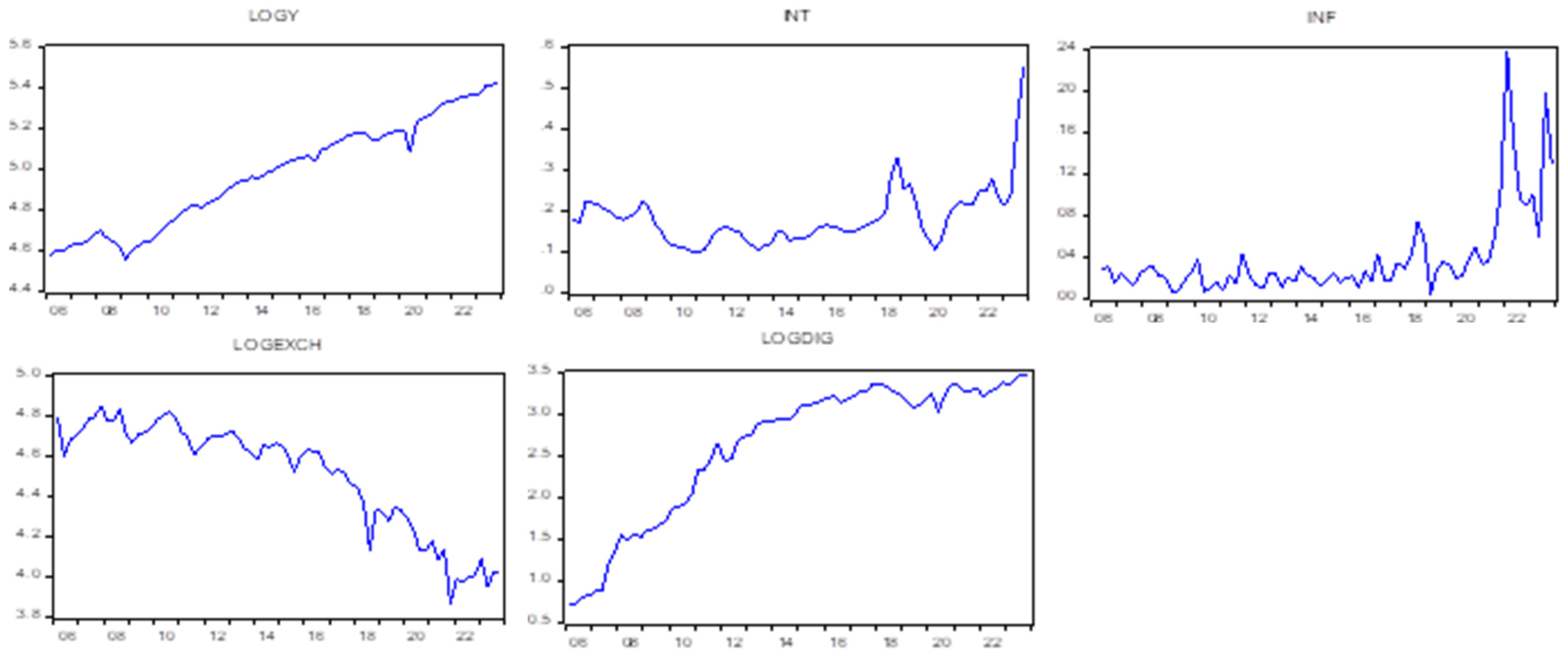
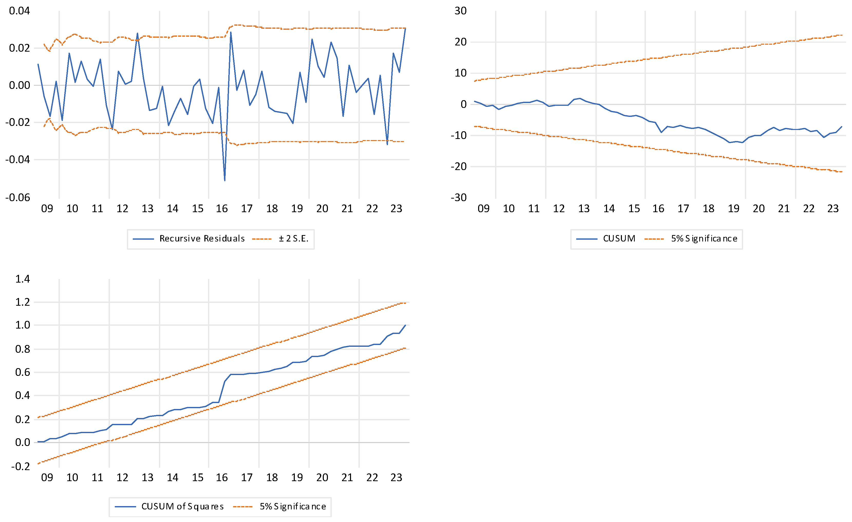
Disclaimer/Publisher’s Note: The statements, opinions and data contained in all publications are solely those of the individual author(s) and contributor(s) and not of MDPI and/or the editor(s). MDPI and/or the editor(s) disclaim responsibility for any injury to people or property resulting from any ideas, methods, instructions or products referred to in the content. |
© 2025 by the authors. Licensee MDPI, Basel, Switzerland. This article is an open access article distributed under the terms and conditions of the Creative Commons Attribution (CC BY) license (https://creativecommons.org/licenses/by/4.0/).