Article

Application of a Small Unmanned Aerial System to Measure Ammonia Emissions from a Pilot Amine-CO2 Capture System

1
Department of Chemistry, University of Kentucky, Lexington, KY 40506, USA
2
Center for Applied Energy Research, University of Kentucky, Lexington, KY 40511, USA
3
Department of Mechanical Engineering, University of Kentucky, Lexington, KY 40506, USA
*
Author to whom correspondence should be addressed.
Sensors 2020, 20(23), 6974; https://doi.org/10.3390/s20236974
Submission received: 17 October 2020 / Revised: 1 December 2020 / Accepted: 4 December 2020 / Published: 6 December 2020
(This article belongs to the Special Issue Sensors for Unmanned Aircraft Systems and Related Technologies)

Abstract

:
The quantification of atmospheric gases with small unmanned aerial systems (sUAS) is expanding the ability to safely perform environmental monitoring tasks and quickly evaluate the impact of technologies. In this work, a calibrated sUAS is used to quantify the emissions of ammonia (NH3) gas from the exit stack a 0.1 MWth pilot-scale carbon capture system (CCS) employing a 5 M monoethanolamine (MEA) solvent to scrub CO2 from coal combustion flue gas. A comparison of the results using the sUAS against the ion chromatography technique with the EPA CTM-027 method for the standard emission sampling of NH3 shows good agreement. Therefore, the work demonstrates the usefulness of sUAS as an alternative method of emission measurement, supporting its application in lieu of traditional sampling techniques to collect real time emission data.

1. Introduction

The use of small unmanned aerial systems (sUAS) has expanded significantly in the scientific community over the last few years. Recent studies have demonstrated the usefulness of sUAS for providing novel measurements in the boundary layer that were previously infeasible with existing methods (i.e., ground stations, towers, weather balloons, manned aircraft, satellites) [1,2,3]. These studies illustrate several advantages that motivate the incorporation of sUAS for atmospheric research. The ability to provide nearly instant real-time emission estimates without the traditional lead times that accompany wet-lab analysis, such as ion chromatography (IC), is desirable in environmental and industrial applications. Furthermore, from the operational cost perspective, the total investment needed for the sUAS is far cheaper than that for costly instrumentation with its associated consumables and periodic services [1]. Additionally, from the safety viewpoint, there is considerable risk associated with sampling gases from hard-to-access stacks for off-line analysis, which also require continuous human checks. Thus, through a systematic flight plan sUAS can easily mitigate the previous sampling hazards. The occasional replacement of batteries is the primary upkeep cost of the sUAS, therefore it is a cost-effective technology to purchase and maintain. Because of the widespread pollution of anthropogenic carbon dioxide (CO2), coal-burning powerplants are a relevant case study for the industrial applications of sUAS for the quantification of point source pollution.
Coal burning power plants emit 4.90 × 10³ Tg of carbon dioxide (CO2) a year, accounting for ~21% of all CO2 emitted throughout the United States of America (U.S.A.) in the year 2017 [4]. It is well-known that CO2 gas absorbs infrared radiation and traps heat in the Earth’s atmosphere, working as a greenhouse gas [5]. As a result, continued anthropogenic CO2 pollution increases radiative forcing, leading to an increase in the average global surface temperature [5]. Thus, practical technologies that counteract the projected increase in CO2 emitted are needed, which should not significantly change the existing methods of energy production [6]. There are numerous strategies to mitigate the effect of fossil fuel-burning power plants and counteract pollution due to the constantly amplifying demand for energy in the last few decades [6,7]. An effective way to reduce emissions in existing coal burning power plants is to retroactively fit (retrofit) them with carbon capture systems (CCS) [8,9] which trap and remove CO2 from the flue gas [10]. One successful solution employs a post-combustion treatment of the flue gas via the absorption of the CO2 with a circulating amine solvent, with a potential emission reduction of up to 90% [11,12,13,14,15,16,17]. Many of the 359 coal burning power plants that operate across the U.S.A. [18] can potentially be fitted with CCS technology. Currently, 65 large-scale projects have started retrofitting carbon capture technologies in the U.S.A. [19].
Ammonia (NH3) gas can be produced from a variety of sources, and has been identified in low quantities as a byproduct from amine-based CCS as a result of the oxidative degradation of the absorbing solvent [20,21,22,23,24]. NH3 is a pollutant with undesirable chemical effects in the atmosphere [25], where large levels can promote aerosol chemistry [26], which affects air quality and climate by forming particulates that are detrimental to public health and scatter solar radiation, respectively [27,28]. For example, the presence of NH3 above background levels can change nitrate aerosol chemistry [29]. Therefore, accurately measuring the emissions of NH3(g) from reported sources is of significant importance. Herein, we quantify NH3(g) emissions from a small pilot-scale CCS with a coal-fired flue gas generator using a 5 M (30.0 wt.%) monoethanolamine (MEA) solvent. For this study, we used the UKySonde, a sUAS [1] equipped with a calibrated NH3(g) sensor [2], along with standard gas emission sampling methodology for comparison.

2. Materials and Methods

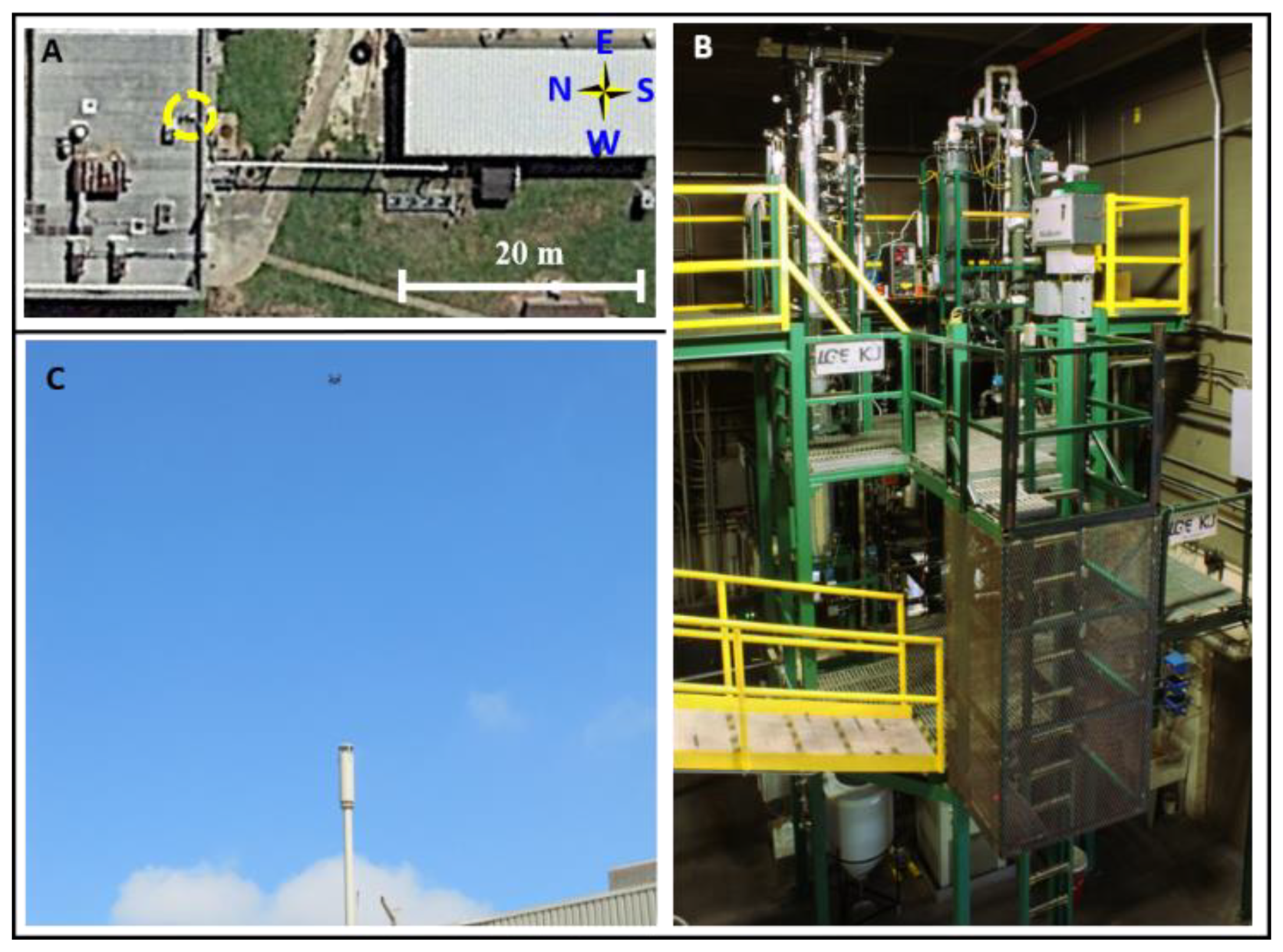
2.1. CO2 Capture System

The University of Kentucky Center for Applied Energy (UKy-CAER) built and operates a bench scale 0.1-megawatt thermal (MWth) CO2 capture system using a coal burning flue gas generator (FGG) to provide representative coal-derived flue gas to the CCS (10–14% CO2, 8–10% O2, other trace gases, and balanced with N2). The UKy-CAER CSS is typically operated during normal working hours in a manner to replicate extreme operation conditions (e.g., high temperatures and contaminate levels) to accelerate solvent degradation and obtain meaningful data form a short operational number of hours. The produced flue gas is transported to the building housing the CCS in the left-hand side of Figure 1a, where 5 M of MEA solvent (in water) is used in a typical aqueous amine-based CCS absorber/regeneration configuration (Figure 1b) to separate the CO2 from the flue gas. Finally, the treated flue gas is released out of a stack (0.194 m diameter), which is in the center of the yellow circle in Figure 1a. All the NH3 concentrations reported from the sUAS readings are measured in close proximity to the stack (as explained below) to model the source point. The scrubbed flue gas typically contains > 2% CO2, along with NH3(g) from the degradation of the amine solvent. The NH3(g) concentration is solvent- and regeneration temperature-dependent. The total emissions from this CCS are relatively small and well below thresholds considered significant from an air permitting perspective [30]. The NH3(g) emissions in the scrubbed flue gas were quantified using an sUAS (Figure 1c), with comparison to the daily emission average values collected using a standard stack sampling methodology based on ion chromatography with the method EPA CTM-027 [20,30]. The experiments with the sUAS took place between September 10 and 14, 2018, above the stack exhaust. The measurements of the background NH3(g) mixing ratio, defined in this work as the mole fraction in air [27], were completed at the ground level (away from the coal burning FGG and CCS) on September 10. The NH3(g) mixing ratios above the stack were registered from September 11 to 14, 2018. The bench facility was fully operational on September 10, 11, and 13, 2018. The standard EPA CTM-027 method was used to compare the sUAS measurements and demonstrate the ability of the sUAS to replace conventional measurement techniques.

2.2. Quantification of NH3(g) with the UKySonde

In the sUAS, called the UKySonde, an analytical sensor (MICS-6814 sensor) is integrated to measure the mixing ratio of NH3 with a 3DR Solo quadcopter from 1 to 2 m above from the stack located at 20 m above ground level (AGL). A 10-bit Arduino UNO microcontroller (Somerville, MA, USA) with a V2 Base Shield (SEEED Studio, Nanshan, China) and an Arduino Wireless SD Shield operating at 5.0 V were used to control the sensing package [2]. Thunder Power batteries with 1350 mA h capacity (RC 2S, Las Vegas, NV, USA) provided the power for data collection, which was set at a rate of 1 Hz, recorded in a SanDisk Ultra Class 10 microSD card with 8 GB capacity (Milpitas, CA, USA). The sensor was calibrated in a custom environmental chamber using standards from 5.00 ppbv to 90.00 ppmv, as described previously [2]. The corresponding linear regression through the origin for this calibration curve is described by Equation (1):
Mixing Ratio of NH3 (ppmv) = 1.0085 × Sensor Response (ppmv).
The performed calibration expanded the operating range of the sensor (from factory specification) to sub-ppmv levels, with an accuracy within ±0.20% of the measured value and a precision of 30 ppbv. Programed flights with Mission Planner Autopilot software were used to monitor the NH3(g) levels at a rate of 1 Hz during operation every 1 h starting at 9 AM (UTC-5). The flights were designed to measure NH3(g) directly from 1 to 2 m above the exhaust stack, corresponding to the maximum mixing ratio in the flue gas after the CCS. The mixing ratios of NH3 reported below for measurements from 1 to 2 m above the stack were corrected after subtracting the average background measured when the fired furnace (located ~60 m downwind) was not operating. Previous work with a tethered balloon equipped with the same sensor package discarded any prop-wash effect by the quadcopter simultaneously measuring NH3 for altitudes between 10 and 120 m above the ground level [2]. The sensor was allowed to warm-up and equilibrate for at least 1 h before take-off operation of programed flights with Mission Planner Autopilot. The flight plan was programed to reach an altitude of 140 m AGL, travel horizontally to the top of the stack position, descend to an altitude of 21 m AGL, and registering data for reporting during the ascent from 21 to 22 m AGL (from 1 to 2 m above the top of the exhaust stack). For data recovery, the device was powered down before removing the SD card.

2.3. Conventional Ammonia Emission Sampling

Ammonia emissions were collected by adapting the methodology from U.S.A. EPA CTM-027 to the facilities 7.62 cm diameter flue gas exit pipe, designed for this purpose, within the CCS. In this method, gaseous ammonia is withdrawn from the CCS exit stack and collected in an aqueous dilute sulfuric acid solution inside a four impinger train connected to a pump (flow rate of 4 L min−1) and metering console. Sulfuric acid was purchased (VWR, Wayne, PA, USA) pre-diluted to the target concentration of 0.05 M. The impinger solutions were combined and stored at 4 °C prior analysis. The method typically samples > 500 L of gas for each sample, with an average of around 600 L of gas and a collection time of 2 h. Field blanks were collected in parallel during the sample collection period as a measure of quality control and ambient ammonia levels and were always below the analytical detection limit. Ammonia absorbed into the sulfuric acid impinger solutions was analyzed by ion chromatography (IC). The samples were diluted with 18.2 MΩ cm−1 water and analyzed by cation ion chromatography using a Dionex ICS-3000 system with an AS autosampler (Dionex-Thermo Scientific, Sunnyvale, CA, USA). The cation IC system consisted of a CSRS 300 suppressor, EGC III MSA (methanesulfonic acid, MSA) eluent generator, IonPac CS17 analytical column and a CG17 guard column operated at 30 °C. The conductivity detector was maintained at 35 °C with a sample injection volume of 20 μL. An isocratic mobile phase of MSA (2.5 mM) at a flow rate of 0.8 mL min−1 was used. Ammonia quantitation used a calibration curve made from a stock ammonium (NH4+) solution (Environmental Express, Charleston, SC, USA). Peak identification and integration was performed manually using the Dionex Chromeleon chromatography management system software version 6.80. Each sample was analyzed in triplicate and the average value was used to calculate the gas phase analyte concentration in ppmv [30]. The method typically requires ~2 h for sample collection and ~1 h for actual analysis per sample.

2.4. Emission Estimates of NH3(g)

The mixing ratio of NH3 (in ppmv), measured immediately above the exhaust stack, were integrated over time and combined with the flow rate of the treated flue gas at the exhaust of ~14.7 actual cubic feet per minute (acfm) to obtain the mass flow of emissions with the industry standard of pounds of NH3 per day (lbs day−1). The average mass flow measured for each flight 1 m above the exhaust stack was fed into a Gaussian plume model to retrieve the mixing ratio inside the stack prior to diffusion. For this model, the atmospheric conditions were neutral, and the exit velocity and temperature of the flue gas were 0.232 m s−1 and 40 °C, respectively. The specific wind inputs for each flight were provided by the nearest weather station (KKYGEORG28) at Horse Country, ~3.2 km away [31].

3. Results and Discussion

The UKySonde flew every ~1 h during 8 h from 11 to 14 September 2018, measuring the NH3(g) levels from the flue gas after treatment with MEA in the CCS on September 11 and 13, and the background levels (with the furnace off) on September 12 and 14. The NH3(g) mixing ratio attributed to the UKy-CAER CCS can be retrieved from the average mixing ratio of NH3 measured in close proximity to the stack throughout the day. The measurement of NH3(g) in the flue gas using the standard stack sampling method took place under generally the same CCS operating conditions, but not in parallel with sUAS sampling. Daily averages of NH3(g) emissions were quantified and used to compare with the sUAS measurements.

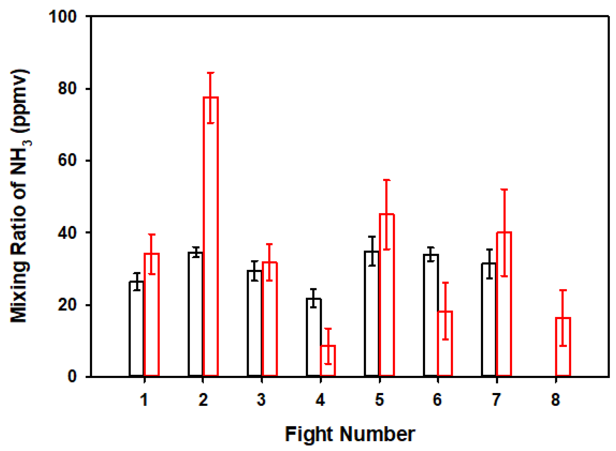
3.1. Ammonia Measurements

The background mixing ratio determined between 12 and 4 pm on September 10th, was 7.26 (±0.35) ppbv. Figure 2 shows the measurements of NH3(g) on 11 and 13 September, which took place every 1 h. The average mixing ratios of NH3 1 m above the stack (at the virtual point source) was 28.90 (±7.60) ppmv on September 11 (black columns in Figure 2). Similarly, during September 13 (red columns in Figure 2), the average 26.70 (±8.80) ppmv NH3(g). On 12 and 14 September, the CCS was not operational, and the flights completed with the UKySonde measured a background mixing ratio 1 m above the exhaust stack, near the low calibration limit of 6.93 (±2.28) and 6.95 (±1.57) ppbv NH3(g), respectively.

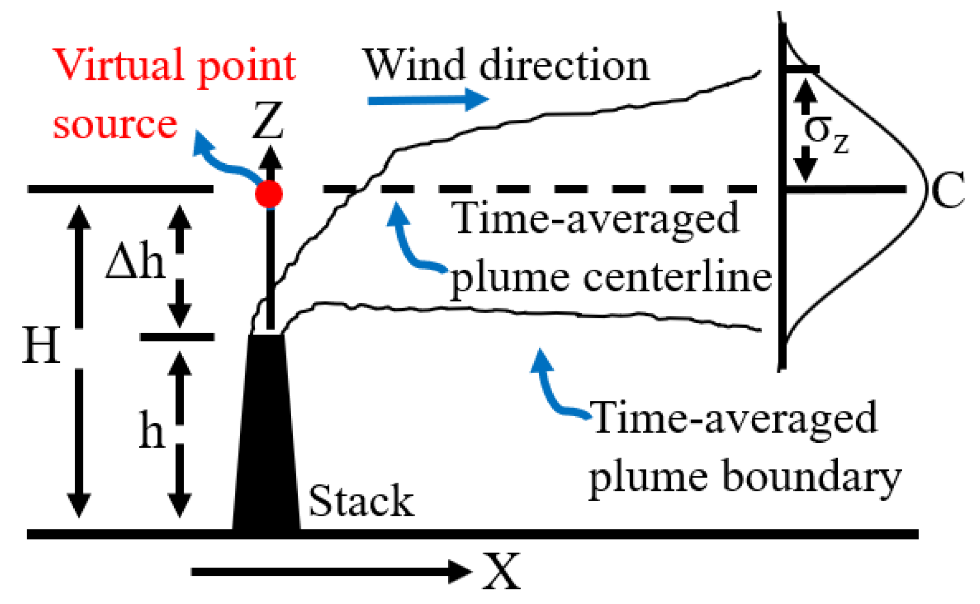
3.2. Gaussian Modeling of the Point Source

The average mixing ratio measured in each flight (Figure 2) was fed into a Gaussian plume model to retrieve the mixing ratio inside the stack prior to diffusion. The Gaussian plume model was chosen to estimate the concentration inside the stack based on measurements taken by the sUAS ~1 m above the stack exit [32,33,34,35]. The model was chosen due to its proven performance over small distances. In other words, this model has been used on small scales on many occasions and successfully modeled the dispersion of gas molecules [36,37,38]. The model was effectively applied to NH3(g), as the measurements of this pollutant were completed under stable meteorological conditions for a short distance in less than 1 h, which is much shorter than its atmospheric lifetime, τ NH 3 ( g ) = 1 day [28,39].
The diffusion of flue gas from the exhaust stack to the NH3(g) sensor depends on many factors, including the emission rate, distance from source, and atmospheric conditions that influence plume characteristics. The most significant atmospheric conditions considered are wind speed, wind direction, and boundary layer stability, all parametrized in the Gaussian plume model to analytically retrieve the original point source concentration. The estimated NH3(g) emission uncertainly is propagated through the sUAS measurements and carried into the model. The overall uncertainty of the measurements is propagated to the final output of the model.
The Gaussian plume model makes the following five assumptions: (1) continuous emission with negligible background pollution; (2) chemical stability, mass conservation after surface contact and negligible deposition; (3) steady-state meteorological conditions, negligible change in wind speed and direction with time and altitude; (4) dispersion parameters are a function of horizontal distance, negligible diffusion in the direction of travel; and (5) the topography does not alter the plume.
The Gaussian dispersion Equation (2) provides the concentration, qe, which depends mainly on the initial flux determined by the UKySonde, Fe, the wind speed oriented along the x-axis, u, and CCS flow rates, and the dispersion coefficients, σy and σz in the respective directions y (horizontal and perpendicular to x) and z (vertical to x), which define the spread of the plume. As for any normal distribution, a 67% of the emitted plume of NH3(g) falls within ±σy and ±σz in each direction. The stable atmospheric conditions during all measurements are properly fit with small dispersion coefficient values. Thus, as the x-axis is defined in the direction of the wind associated with the diffusion coefficient σx, the horizontal σy is largely dependent on crosswinds of variable speed and direction in the y-axis. The vertical distance from the source, relative to the point source height, represented in the z direction in Figure 3, is associated with a vertical diffusion coefficient, σz, which varies with temperature gradients. Stable atmospheric conditions reduce diffusion, resulting in small σz values.
q e = F e 2 π σ y σ z u exp ( ( y ) 2 2 σ y 2 ) { exp ( ( z     H ) 2 2 σ z 2 ) + exp ( ( z   +   H ) 2 2 σ z 2 ) } .
Table 1 shows the input parameters used in the model for each flight, where the indicated input NH3 (ppmv) was used to retrieve the flux of the emitted NH3 (µg/s) needed at the point source to create the measured amounts at the virtual point (1 m above). The flux emitted was finally converted into a model mixing ratio in ppmv units. For the previous purpose, the exit gas velocity transported through the fixed stack surface area at the exhaust was needed. As an example of the data treatment for the flights, the model ran with atmospheric conditions that were neutral, and the exit velocity and temperature of the flue gas were 0.232 m s−1 and 40 °C, respectively. The stack diameter was 0.194 m. The specific wind inputs and ambient air temperatures for each flight were provided by the nearest weather station (KKYGEORG28) at Horse Country, ~3.2 km away. The wind speed for each flight was constant (e.g., for the first flight on September 11 it was consistently at 7 mph NE, with a temperature of 20.0 °C (Table 1)). The Gaussian plume model run as a function of distance from the stack (~ 1 m) was used to estimate the typical σy and σz values. The wind speed on September 11 was consistent for all flights, except for flight 4, which slowed down by less than 5%. Instead, the windspeeds on September 13, although lower than for September 11, varied by 52% among the eight flights. This variance in wind speed affecting plume dispersion contributed the most significant source of uncertainty introduced by the model. Table 1 also sows the results of converting the output mixing ratio in ppmv units into an emission flux with units of lbs/day.
The quantification of the NH3(g) in air above the exhaust stack is not affected by any chemical transformations during the short distance from the exit orifice and the time scale of measurements. However, in addition to physical variability—i.e., provided by wind speed and temperature—the sensor registers any fluctuations in the NH3(g) emitted due to changes in the chemical composition of the treated flue gas due to dynamic MEA decomposition reactions. Thus, although the exit gas velocity from the exhaust stack in Table 1 remains constant, the composition of gas varies as recorded by the UKySonde measurements combined with the Gaussian plume model.

3.3. Comparison of NH3(g) Emissions Measurement Techniques

Table 1 also displays the model output data for each flight in Figure 1, which indicate that the average mixing ratios of NH3 measured at the virtual point during September 11 and 13, 28.90 (±7.60) ppmv and 26.70 (±8.80) ppmv, correspond to the mixing ratios at the point source (inside the stack) of 80.30 (±10.10) ppmv and 82.00 (±13.30) ppmv, respectively. The retrieved mixing ratios from the modeled UKySonde measurements are in close agreement with the ion chromatography results of seven samples collected in the exhaust from the CCS, which were in the range from 11.90 to 120.0 ppmv, with an average of 84.40 (±18.00) ppmv. In addition, the retrieved point source mixing ratios can be easily converted to emission rates of 7.20 (±0.93) × 10−3 and 7.55 (±1.23) × 10−3 lbs day−1 of NH3(g) on September 11 and 13, respectively.
The mixing ratio of NH3 was measured with two independent analytical methods, providing quality assurance of the similar NH3(g) emission reported by the UKySonde and the standard stack sampling method during the operation of the CCS. The combined sUAS method with the Gaussian plume model determined an average NH3 mixing ratio of 81.20 (±16.70) ppmv in the flue gas, while conventional gas sampling measured an average of 84.40 (±18.00) ppmv. Both values agreed reasonably well within the experimental errors expected from two different analytical techniques. These measured values are also comparable to published ammonia emission values from the MEA testing campaigns at other CCS units of variable size and flue gas composition [30]. The overlapping results of the emission estimates from the traditional sampling methods and the sUAS further supports their use in quantifying industrial point source pollution. This work demonstrates that the integration of sUAS into routine emission sampling can provide accurate, real-time results and can be a valid alternative to wet-lab techniques.

4. Conclusions

Several advantages and disadvantages can be considered for applying the sUAS method in this work for determining NH3(g) emissions as compared to the traditional offline EPA ion chromatography sampling method. The new method is cheap and easy to implement while providing a faster measurement and sampling frequency than ion chromatography. In addition, the use of a sUAS eliminates the risk to human life associated with sample collection requiring the climbing of hard-to-access exhaust stacks emitting toxic pollutants. However, the use of a sUAS requires access to meteorological information or the ability to register it. In this context and as a disadvantage, other atmospheric regimes than the one studied here would require the implementation of alternative dispersion models and in situ wind measurements. The implementation of the technique also requires a licensed sUAS pilot and appropriate flying authorizations. A final potential advantage of the sUAS is to allow for the simultaneous sampling of other pollutants with appropriate sensor probes and emission parameters by including sonic anemometers for determining wind speed and direction and physical parameters (temperature, pressure, and relative humidity).
Currently, the total annual NH3(g) emissions in the U.S.A. is 3.0 (± 0.2) Tg year−1, with 70–80% attributed to agriculture (e.g., fertilizer and manure) and the remaining 20–30% originating from industry and other anthropogenic sources [40]. Having the ability to quickly measure NH3(g) emissions from a point source, such as this amine-based CCS, has broad implications and is a potential application of this technique. The ability to record essentially real-time emission data is of significant interest to utility and industrial locations, in addition to regulatory agencies. Overall, this work demonstrates that NH3(g) emissions can be estimated with confidence using sUAS and are a viable option to replace existing sampling methods. The use of sUAS as an analytical tool to quantify point source anthropogenic pollution NH3(g) can find application also in natural settings. In this regard, future work could be expanded by performing horizontal flight patterns with in situ wind measurements to characterize the plume completely as it traverses the boundary layer and undergoes atmospheric ageing. Possible interesting efforts in this field could also include numerical simulations to compare with present or new measured results. Particularly, the recent development of computational fluid dynamics (CFD) numerical simulations can contribute to improve the analysis of pollutant emissions and their spread [41,42]. Finally, this work also serves as an example for future applications of sUAS to monitor pollution emissions—i.e., in the case of agriculture and ammonia contributed by livestock or from rice paddies.

Author Contributions

M.I.G. proposed the idea for this work; M.I.G., J.G.T., and K.L. provided the materials and made suggestions throughout the process; T.J.S. assembled the sensor systems, performed all the flights, and analyzed the data; B.I. operated the CCS system; K.A. collected the emission samples and performed IC analyses; M.I.G. and T.J.S. wrote the original draft. All the authors revised and approved the manuscript. All authors have read and agreed to the published version of the manuscript.

Funding

NASA funding through an R3 EPSCoR award (80NSSC19M0032) and a Kentucky Space Grant Graduate Fellowship award (NNX15AR69H) provided partial support for this research. The APC was funded by MDPI Sensors.

Acknowledgments

M.I.G. thanks NASA for funding through an R3 EPSCoR award (80NSSC19M0032) and a Kentucky Space Grant Graduate Fellowship award (NNX15AR69H) to partially support T.J.S. UK-CAER acknowledges the Carbon Management Research Group (CMRG) members, including Louisville Gas & Electric (LG&E) and Kentucky Utilities (KU), Duke Energy, American Electric Power (AEP), and Electric Power Research Institute (EPRI) for their financial support in constructing the pilot CCS. We thank the three anonymous reviewers whose comments and suggestions helped improve and clarify the manuscript.

Conflicts of Interest

The authors declare no conflict of interest. The funders had no role in the design of the study, or interpretation of data; in the writing of the manuscript, or in the decision to publish this material.

References

  1. Schuyler, T.J.; Guzman, M.I. Unmanned aerial systems for monitoring trace tropospheric gases. Atmosphere 2017, 8, 206. [Google Scholar] [CrossRef] [Green Version]
  2. Schuyler, T.J.; Bailey, S.C.; Guzman, M.I. Monitoring Tropospheric Gases with Small Unmanned Aerial Systems (sUAS) during the Second CLOUDMAP Flight Campaign. Atmosphere 2019, 10, 434. [Google Scholar] [CrossRef] [Green Version]
  3. Schuyler, T.J.; Gohari, S.M.I.; Pundsack, G.; Berchoff, D.; Guzman, M.I. Using a Balloon-Launched Unmanned Glider to Validate Real-Time WRF Modeling. Sensors 2019, 19, 1914. [Google Scholar] [CrossRef] [PubMed]
  4. Environmental Protection Agency. Inventory of U.S. Greenhouse Gas Sinks; Environmental Protection Agency: Washington, DC, USA, 2019; pp. 71–86.
  5. Environmental Protection Agency. Climate Change Indicators in The United States, 4th ed.; Environmental Protection Agency: Washington, DC, USA, 2016; pp. 12–20.
  6. Environmental Protection Agency. Energy Efficienty as a Low-Cost Resource for Achieving Carbon Emissions Reductions; Environmental Protection Agency: Washington, DC, USA, 2009.
  7. Davies, K.; Malik, A.; Li, J.; Aung, T.N. A meta-study on the feasibility of the implementation of new clean coal technologies to existing coal-fired power plants in an effort to decrease carbon emissions. Energy Sci. Technol. 2017, 4, 30–45. [Google Scholar] [CrossRef] [Green Version]
  8. Zhao, M.; Minett, A.I.; Harris, A.T. A review of techno-economic models for the retrofitting of conventional pulverised-coal power plants for post-combustion capture (PCC) of CO2. Energy Environ. Sci. 2013, 6, 25–40. [Google Scholar] [CrossRef]
  9. Chung, T.S.; Patiño-Echeverri, D.; Johnson, T.L. Expert assessments of retrofitting coal-fired power plants with carbon dioxide capture technologies. Energy Policy 2011, 39, 5609–5620. [Google Scholar] [CrossRef]
  10. Mondal, M.K.; Balsora, H.K.; Varshney, P. Progress and trends in CO2 capture/separation technologies: A review. Energy 2012, 46, 431–441. [Google Scholar] [CrossRef]
  11. Wang, M.; Lawal, A.; Stephenson, P.; Sidders, J.; Ramshaw, C. Post-combustion CO2 capture with chemical absorption: A state-of-the-art review. Chem. Eng. Res. Des. 2011, 89, 1609–1624. [Google Scholar] [CrossRef] [Green Version]
  12. Singh, B.; Strømman, A.H.; Hertwich, E. Life cycle assessment of natural gas combined cycle power plant with post-combustion carbon capture, transport and storage. Int. J. Greenh. Gas Control 2011, 5, 457–466. [Google Scholar] [CrossRef]
  13. Conway, W.; Wang, X.; Fernandes, D.; Burns, R.; Lawrance, G.; Puxty, G.; Maeder, M. Comprehensive kinetic and thermodynamic study of the reactions of CO2 (aq) and HCO3 with monoethanolamine (MEA) in aqueous solution. J. Phys. Chem. A 2011, 115, 14340–14349. [Google Scholar] [CrossRef]
  14. Lv, B.; Guo, B.; Zhou, Z.; Jing, G. Mechanisms of CO2 capture into monoethanolamine solution with different CO2 loading during the absorption/desorption processes. Environ. Sci. Technol. 2015, 49, 10728–10735. [Google Scholar] [CrossRef] [PubMed]
  15. Puxty, G.; Rowland, R.; Attalla, M. Comparison of the rate of CO2 absorption into aqueous ammonia and monoethanolamine. Chem. Eng. Sci. 2010, 65, 915–922. [Google Scholar] [CrossRef]
  16. Qin, F.; Wang, S.; Hartono, A.; Svendsen, H.F.; Chen, C. Kinetics of CO2 absorption in aqueous ammonia solution. Int. J. Greenh. Gas Control 2010, 4, 729–738. [Google Scholar] [CrossRef]
  17. Rao, A.B.; Rubin, E.S. A technical, economic, and environmental assessment of amine-based CO2 capture technology for power plant greenhouse gas control. Environ. Sci. Technol. 2002, 36, 4467–4475. [Google Scholar] [CrossRef] [PubMed] [Green Version]
  18. U.S. Energy Information Administration. Electric Power Annual 2017; U.S. Energy Information Administration: Washington, DC, USA, 2019.
  19. Scott, V.; Gilfillan, S.; Markusson, N.; Chalmers, H.; Haszeldine, R.S. Last chance for carbon capture and storage. Nat. Clim. Chang. 2013, 3, 105. [Google Scholar] [CrossRef] [Green Version]
  20. Thompson, J.G.; Bhatnagar, S.; Combs, M.; Abad, K.; Onneweer, F.; Pelgen, J.; Link, D.; Figueroa, J.; Nikolic, H.; Liu, K. Pilot testing of a heat integrated 0.7 MWe CO2 capture system with two-stage air-stripping: Amine degradation and metal accumulation. Int. J. Greenh. Gas Control 2017, 64, 23–33. [Google Scholar] [CrossRef]
  21. Chi, S.; Rochelle, G.T. Oxidative degradation of monoethanolamine. Ind. Eng. Chem. Res. 2002, 41, 4178–4186. [Google Scholar] [CrossRef]
  22. da Silva, E.F.; Lepaumier, H.; Grimstvedt, A.; Vevelstad, S.J.; Einbu, A.; Vernstad, K.; Svendsen, H.F.; Zahlsen, K. Understanding 2-ethanolamine degradation in postcombustion CO2 capture. Ind. Eng. Chem. Res. 2012, 51, 13329–13338. [Google Scholar] [CrossRef]
  23. Goff, G.S.; Rochelle, G.T. Monoethanolamine degradation: O2 mass transfer effects under CO2 capture conditions. Ind. Eng. Chem. Res. 2004, 43, 6400–6408. [Google Scholar] [CrossRef]
  24. Ma, S.; Song, H.; Wang, M.; Yang, J.; Zang, B. Research on mechanism of ammonia escaping and control in the process of CO2 capture using ammonia solution. Chem. Eng. Res. Des. 2013, 91, 1327–1334. [Google Scholar] [CrossRef]
  25. Kirkby, J.; Curtius, J.; Almeida, J.; Dunne, E.; Duplissy, J.; Ehrhart, S.; Franchin, A.; Gagné, S.; Ickes, L.; Kürten, A. Role of sulphuric acid, ammonia and galactic cosmic rays in atmospheric aerosol nucleation. Nature 2011, 476, 429. [Google Scholar] [CrossRef] [PubMed]
  26. Luo, C.; Zender, C.S.; Bian, H.; Metzger, S. Role of ammonia chemistry and coarse mode aerosols in global climatological inorganic aerosol distributions. Atmos. Environ. 2007, 41, 2510–2533. [Google Scholar] [CrossRef] [Green Version]
  27. Jacob, D.J. Introduction to Atmospheric Chemistry; Princeton University Press: Princeton, NJ, USA, 1999. [Google Scholar]
  28. Seinfeld, J.H.; Pandis, S.N. Atmospheric Chemistry and Physics: From Air Pollution to Climate Change, 3rd ed.; John Wiley & Sons: Hoboken, NJ, USA, 2016; p. 1152. [Google Scholar]
  29. Paulot, F.; Ginoux, P.; Cooke, W.; Donner, L.; Fan, S.; Lin, M.-Y.; Mao, J.; Naik, V.; Horowitz, L. Sensitivity of nitrate aerosols to ammonia emissions and to nitrate chemistry: Implications for present and future nitrate optical depth. Atmos. Chem. Phys. 2016, 16, 1459–1477. [Google Scholar] [CrossRef] [Green Version]
  30. Thompson, J.G.; Combs, M.; Abad, K.; Bhatnagar, S.; Pelgen, J.; Beaudry, M.; Rochelle, G.; Hume, S.; Link, D.; Figueroa, J. Pilot testing of a heat integrated 0.7 MWe CO2 capture system with two-stage air-stripping: Emission. Int. J. Greenh. Gas Control 2017, 64, 267–275. [Google Scholar] [CrossRef]
  31. Weather Underground Inc. Horse Country Weather Station (KKyLEXIN183). Available online: https://www.wunderground.com/dashboard/pws/KKYGEORG28/graph/2018-09-16/2018-09-16/weekly (accessed on 20 September 2018).
  32. Brusca, S.; Famoso, F.; Lanzafame, R.; Mauro, S.; Garrano, A.M.C.; Monforte, P. Theoretical and Experimental Study of Gaussian Plume Model in Small Scale System. Energy Procedia 2016, 101, 58–65. [Google Scholar] [CrossRef]
  33. De Nevers, N. Air Pollution Control Engineering, 2nd ed.; Waveland Press Inc.: Long Grove, IL, USA, 2010. [Google Scholar]
  34. Stockie, J.M. The Mathematics of Atmospheric Dispersion Modeling. Siam Rev. 2011, 53, 349–372. [Google Scholar] [CrossRef]
  35. Turner, B.D. Workbook of Atmospheric Dispersion Estimates: An Introduction to Dispersion Modeling; CRC Press: Boca Raton, FL, USA, 1994. [Google Scholar]
  36. Marjovi, A.; Marques, L. Multi-Robot Odor Distribution Mapping in Realistic Time-Variant Conditions. In Proceedings of the 2014 IEEE International Conference on Robotics and Automation, Hong Kong, China, 31 May–7 June 2014; IEEE: Piscataway, NJ, USA, 2014; pp. 3720–3727. [Google Scholar]
  37. Murlis, J.; Elkinton, J.S.; Carde, R.T. Odor Plumes and How Insects Use Them. Rev. Entomol. 1992, 37, 505–532. [Google Scholar] [CrossRef]
  38. Sánchez-Sosa, J.E.; Castillo-Mixcóatl, J.; Beltrán-Pérez, G.; Muñoz-Aguirre, S. An Application of the Gaussian Plume Model to Localization of an Indoor Gas Source with a Mobile Robot. Sensors 2018, 18, 4375. [Google Scholar] [CrossRef] [Green Version]
  39. Pinder, R.W.; Gilliland, A.B.; Dennis, R.L. Environmental impact of atmospheric NH3 emissions under present and future conditions in the eastern United States. Geophys. Res. Lett. 2008, 35, L12808. [Google Scholar] [CrossRef]
  40. Paulot, F.; Jacob, D.J.; Pinder, R.W.; Bash, J.O.; Travis, K.; Henze, D.K. Ammonia emissions in the United States, European Union, and China derived by high-resolution inversion of ammonium wet deposition data: Interpretation with a new agricultural emissions inventory (MASAGE_NH3). J. Geophys. Res. Atmos. 2014, 119, 4343–4364. [Google Scholar] [CrossRef]
  41. El Bahlouli, A.; Leukauf, D.; Platis, A.; zum Berge, K.; Bange, J.; Knaus, H. Validating CFD Predictions of Flow over an Escarpment Using Ground-Based and Airborne Measurement Devices. Energies 2020, 13, 4688. [Google Scholar] [CrossRef]
  42. El Bahlouli, A.; Rautenberg, A.; Schön, M.; zum Berge, K.; Bange, J.; Knaus, H. Comparison of CFD Simulation to UAS Measurements for Wind Flows in Complex Terrain: Application to the WINSENT Test Site. Energies 2019, 12, 1992. [Google Scholar] [CrossRef] [Green Version]
Figure 1. (A) Aerial view of the facilities employed in the University of Kentucky Center for Applied Energy (UKy-CAER). The coal flue gas generator is located to the right side and the gas flows through a polyvinyl chloride (PVC) pipe (from right to left) to the building on the left-hand side for amine treatment in the carbon capture system (CCS) before the scrubbed flue gas emissions are released out the stack at the top (yellow dashed circle). (B) Image of the amine-based CCS at UKy-CAER. (C) Perspective view of the small unmanned aerial system (sUAS) flying above the stack.
Sensors 20 06974 g001
Figure 2. Mixing ratio of NH3(g) measured 1 m above the exhaust stack every 1 h (from 9:00 AM, UTC-5) by the UKySonde on September 11 (black) and 13 (red) of 2018.
Sensors 20 06974 g002
Figure 3. Schematic representation of the Gaussian plume model utilized to retrieve the mixing ratio of NH3(g) in the exhaust stack from the values measured 1 m above.
Sensors 20 06974 g003
Table 1. Input parameters for the Gaussian plume modeling and results.
DateFlight #Mixing Ratio of NH3(g) (ppmv)Stack Radius (m)Exit Gas Velocity (m/s)Exit Gas Temp (°C)Air Temp (°C)Wind Speed (m/s)Emitted NH3 (µg/s)Model Output NH3(g) (ppmv)NH3(g) Emission
(lbs day−1)
9/11/2018126.28 (±2.40)0.0970.2324020.03.1667686.27 (±0.59) × 10−3
234.54 (±1.43)0.0970.2324020.03.1877908.29 (±0.35) × 10−3
329.38 (±2.81)0.0970.2324020.63.1746777.10 (±0.69) × 10−3
421.73 (±2.58)0.0970.2324021.12.7552655.99 (±0.63) × 10−3
534.82 (±4.07)0.0970.2324021.73.1884918.39 (±1.00) × 10−3
633.96 (±1.81)0.0970.2324021.73.1863898.20 (±0.44) × 10−3
731.34 (±3.97)0.0970.2324020.63.1796827.56 (±0.97) × 10−3
9/13/2018134.09 (±5.50)0.0970.2324028.91.02471059.66 (±0.31) × 10−3
277.50 (±6.94)0.0970.2324030.01.08782382.19 (±0.39) × 10−3
331.67 (±5.00)0.0970.2324031.11.3230756.90 (±0.28) × 10−3
48.53 (±4.91)0.0970.2324031.13.6552100.92 (±0.27) × 10−3
545.00 (±9.57)0.0970.2324031.11.032613812.69 (±0.55) × 10−3
618.18 (±7.89)0.0970.2324031.12.7132211.93 (±0.44) × 10−3
740.00 (±12.08)0.0970.2324029.42.7290464.23 (±0.67) × 10−3
816.28 (±7.71)0.0970.2324026.72.2118232.12 (±0.43) × 10−3
Publisher’s Note: MDPI stays neutral with regard to jurisdictional claims in published maps and institutional affiliations.

