Performance Evaluation of Bluetooth Low Energy: A Systematic Review

 ,
, 

Abstract
:1. Introduction
- Firstly, in Section 2, we describe the main frames and functions of the BLE protocol stack, analyzing in detail how the communication works, how a packet is structured and how the possible network typologies are.
- Then, in Section 3, we systematically review the works available in the literature about the use of BLE, providing a common theoretical framework to discuss in detail the main remarks observed in these studies and defining guidelines for the BLE setting in different conditions of use.
- Finally, in Section 4, we summarize studies on the main characteristics, uses and limits of BLE, trying to define guidelines on what is already consolidated in the literature, what are the open issues and suggesting what could be the next utile investigations on this technology.
2. BLE Functioning
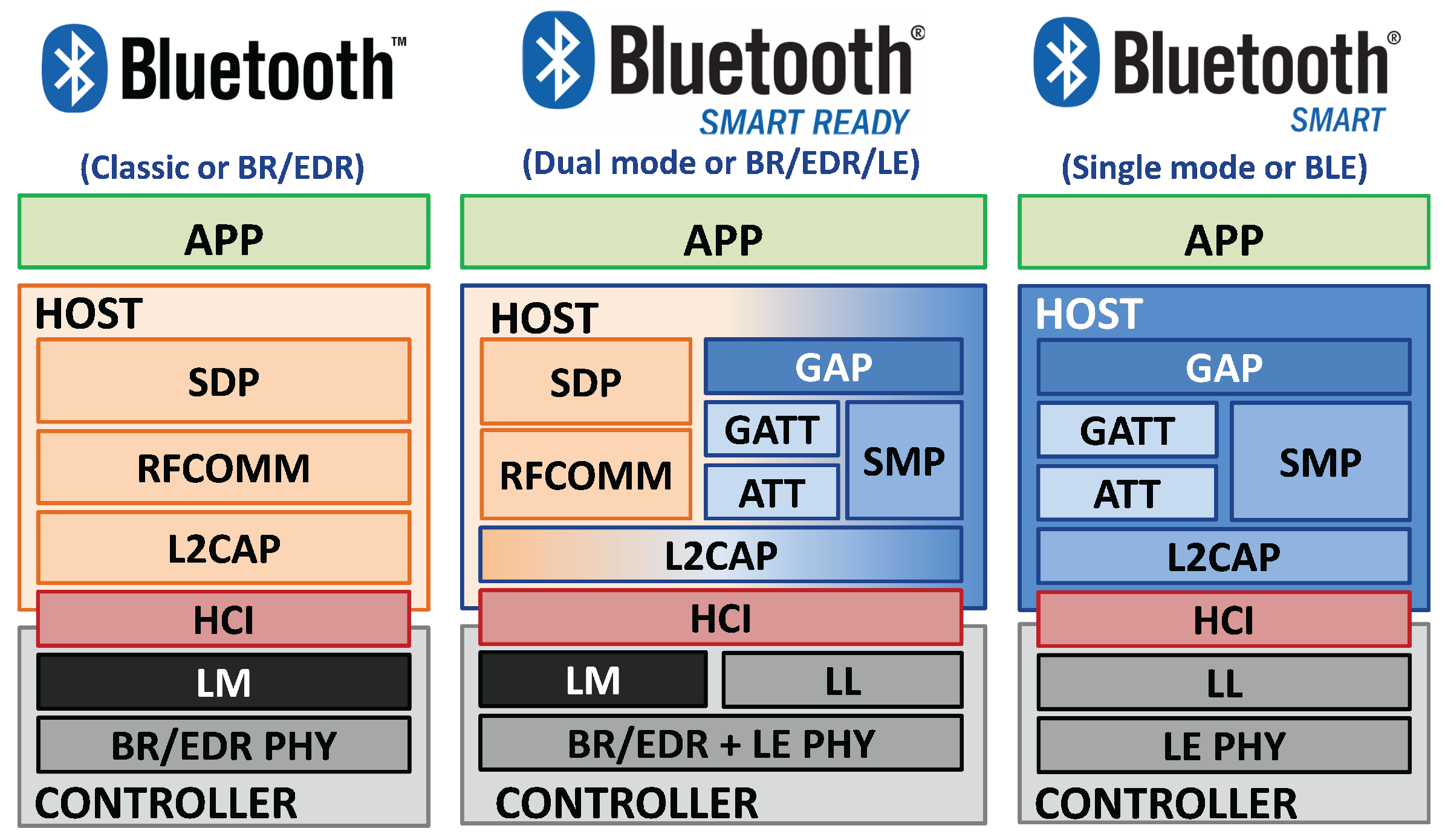
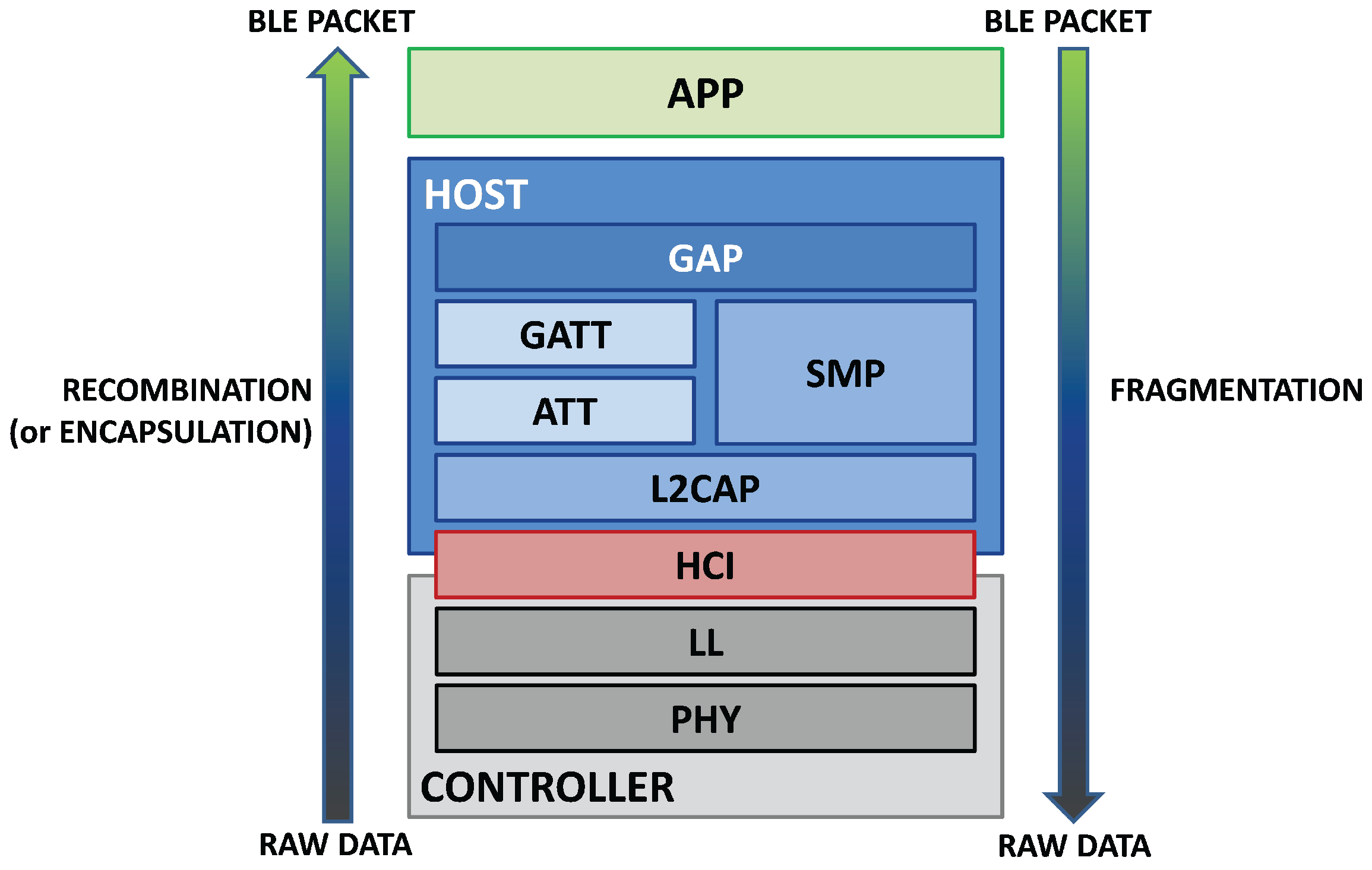
2.1. BLE Protocol Stack
- The Application (App) is the highest block of the stack, and it represents the direct interface with the user. It defines some profiles thanks to which different applications, which reuse common functionality, are able to interoperate. These application profiles are specified by the Bluetooth SIG and encourage interoperability between devices from different manufacturers. Bluetooth specification allows also defining vendor-specific profiles for use cases not covered by the SIG-defined profiles.
- The Host includes the following layers:
- -
- Generic Access Profile (GAP)
- -
- Generic Attribute Profile (GATT)
- -
- Logical Link Control and Adaptation Protocol (L2CAP)
- -
- Attribute Protocol (ATT)
- -
- Security Manager Protocol (SMP)
- -
- Host Controller Interface (HCI), Host side
- The Controller is structured in the following layers:
- -
- Host Controller Interface (HCI), Controller side
- -
- Link Layer (LL)
- -
- Physical Layer (PHY)
2.1.1. Physical Layer
2.1.2. Link Layer
- Preamble, Access Address and air protocol framing.
- Cyclic Redundancy Check (CRC) generation and verification.
- Data whitening.
- Random number generation.
- Advanced Encryption Standard (AES).
2.1.3. Host Controller Interface
2.1.4. Logical Link Control and Adaptation Protocol
2.1.5. Security Manager Protocol
2.1.6. Attribute Protocol
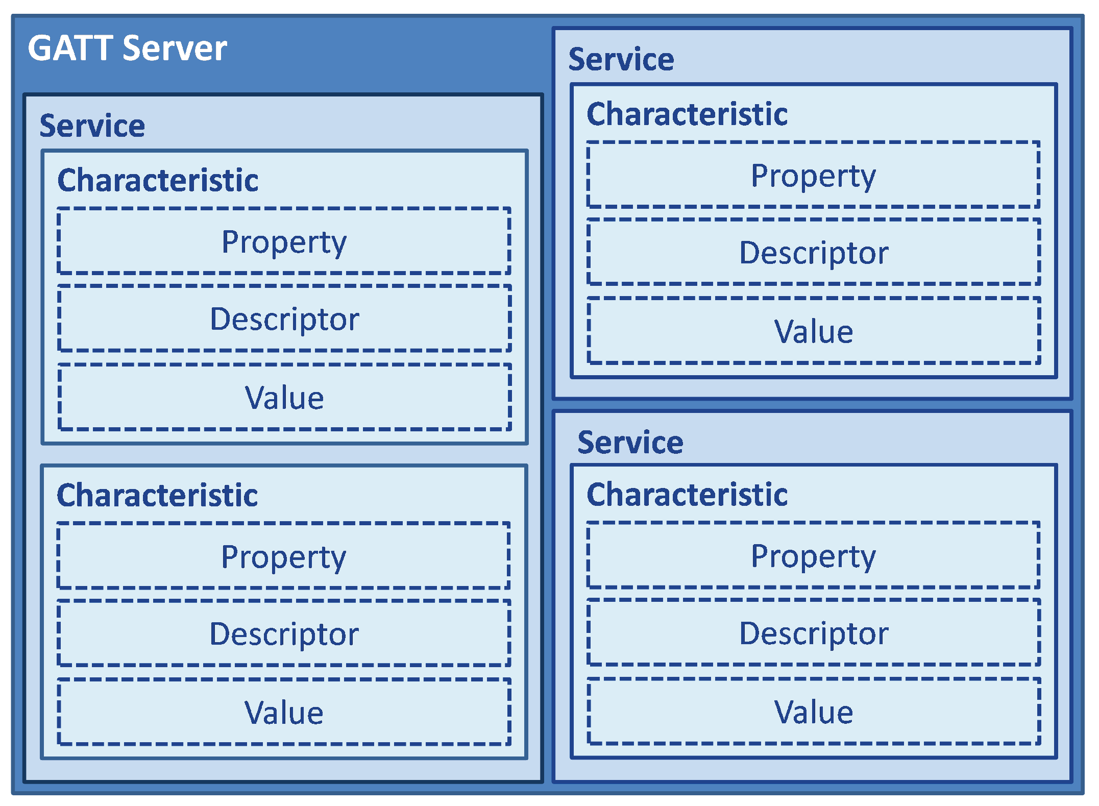
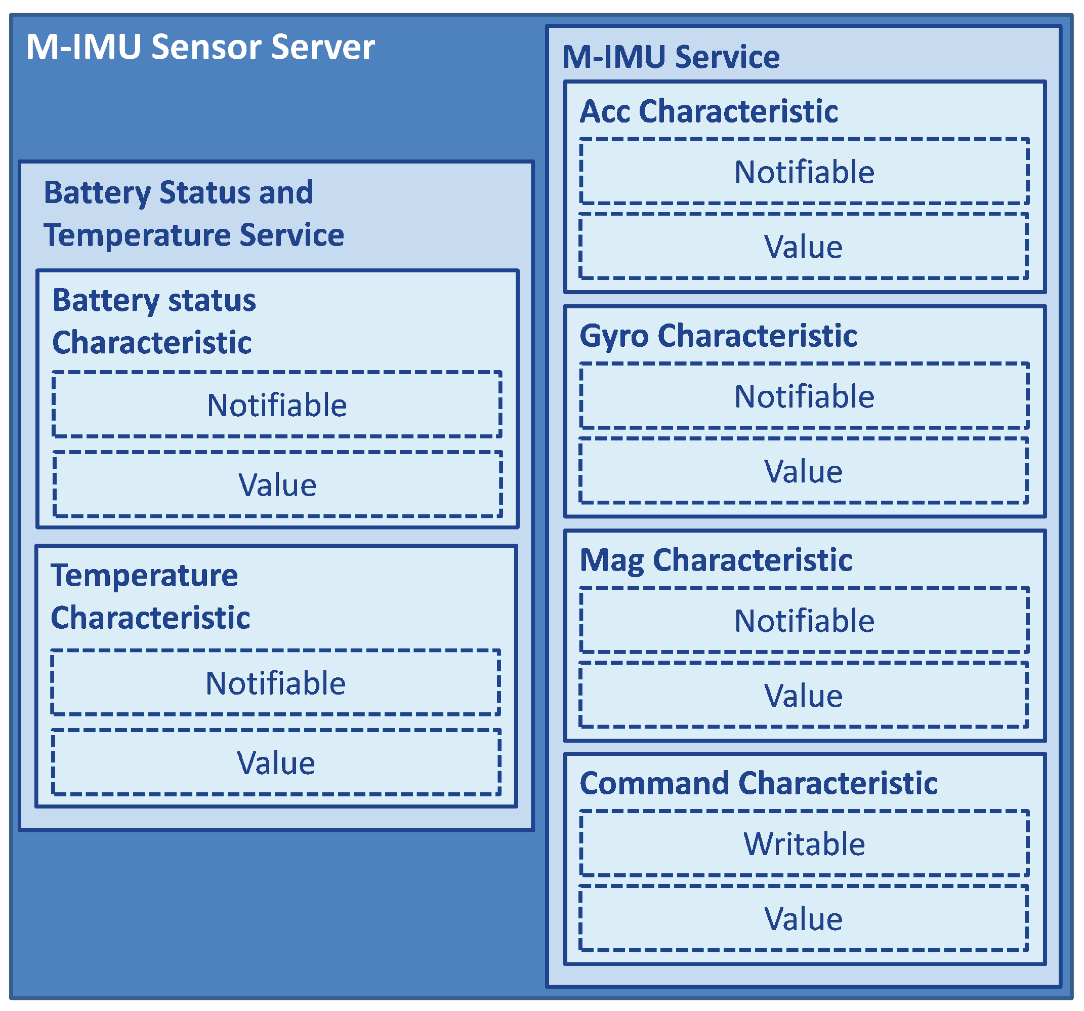
2.1.7. Generic Attribute Profile
- Broadcast: this allows sending data to BLE devices using advertising packets, as described in Section 2.2.1.
- Readable: if set, the client can only read the characteristic value.
- Writable: with this property, the client can only write a new value on the characteristic.
- Notifiable: when it is set, the client receives a notification if the server updates the characteristic, so that it can read the new value.
- M-IMU service: This manages all the data referred to the M-IMU, and it is structured into four different characteristics. Three notifiable characteristics perform the task to send data from the sensor to the central device; one is referred to the accelerometer data, one for the gyroscope and the last one for the magnetometer. The last characteristic is writable so that the central node can modify some properties of the M-IMU, for example the sampling frequency or how many of the three sensors are transmitting.
- Battery Status and Temperature service: This has two notifiable characteristics, used to send data relative to the remaining battery charge and the temperature. In order to preserve energy, it could send data with a rate lower than the one of the service previously described. This is another reason why it is better to correctly manage the GATT logical structure; in this way, it is possible to separate data transmission depending on the specific use.
2.1.8. Generic Access Profile
2.2. BLE Communication
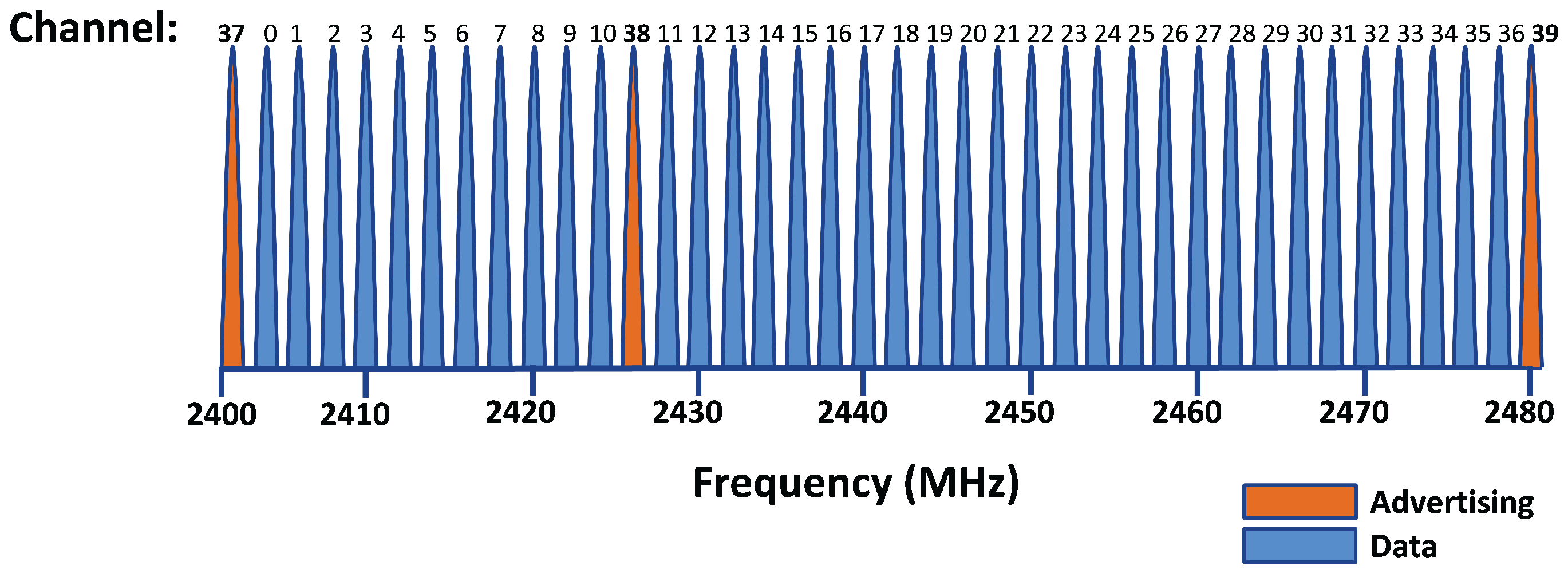
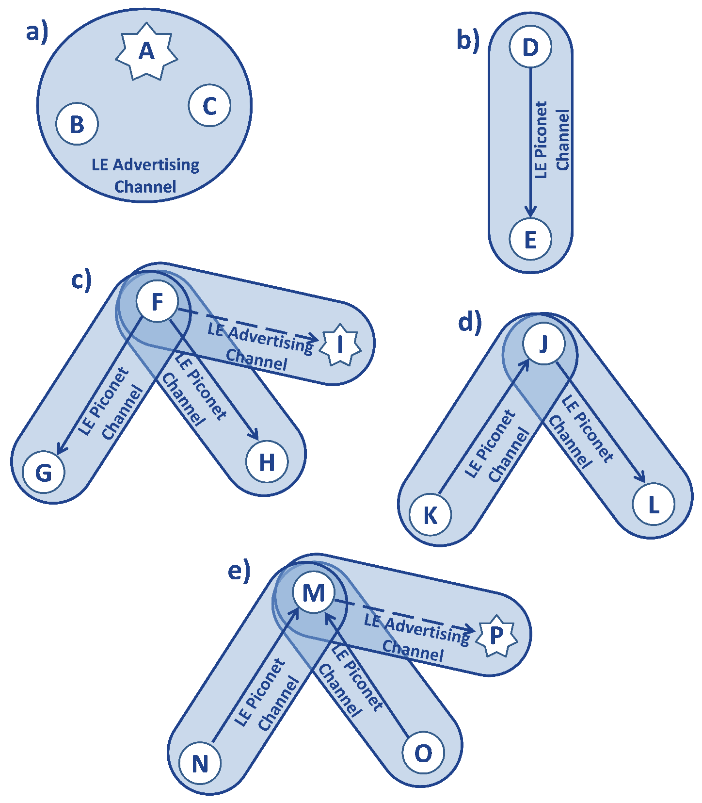
2.2.1. Broadcasting
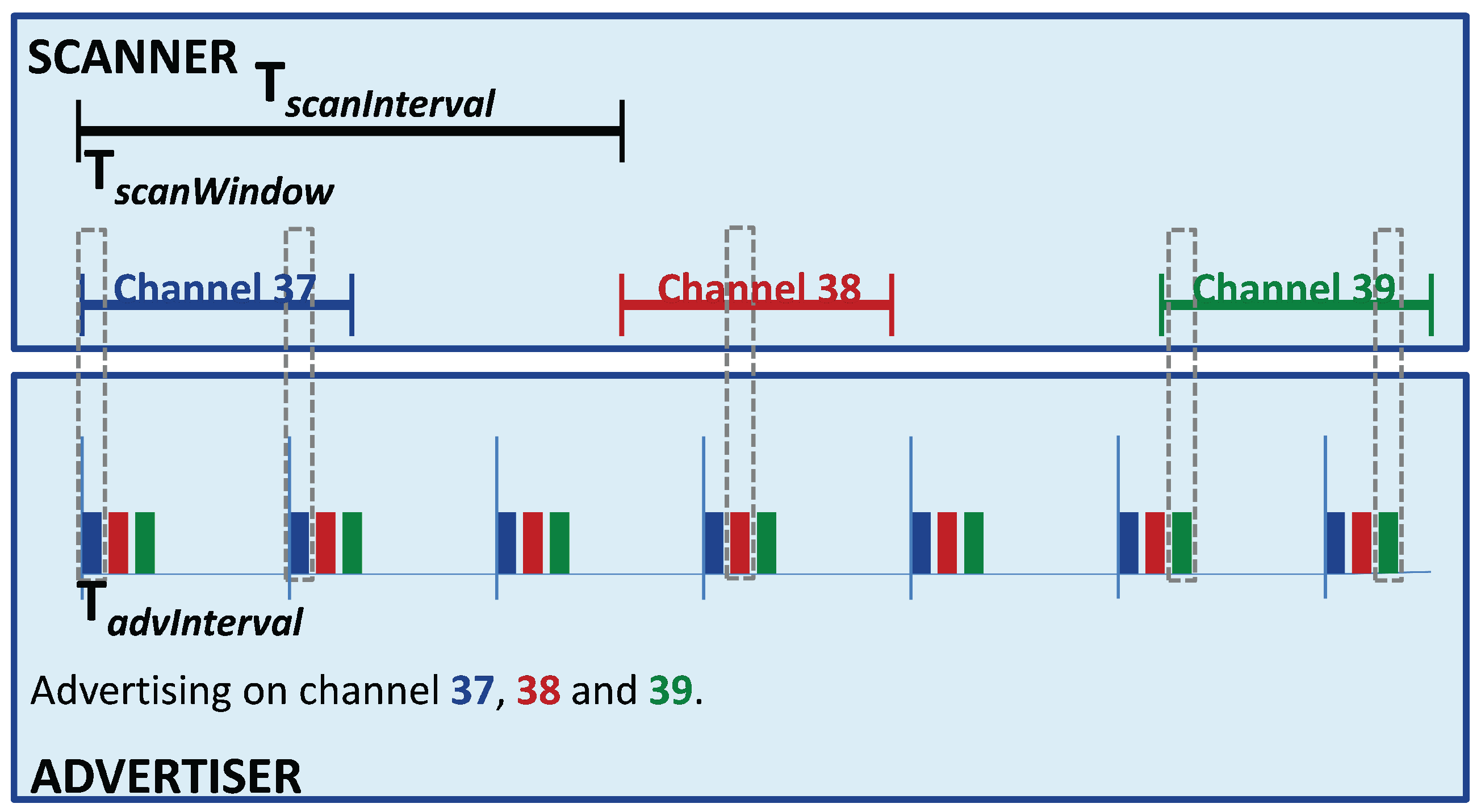
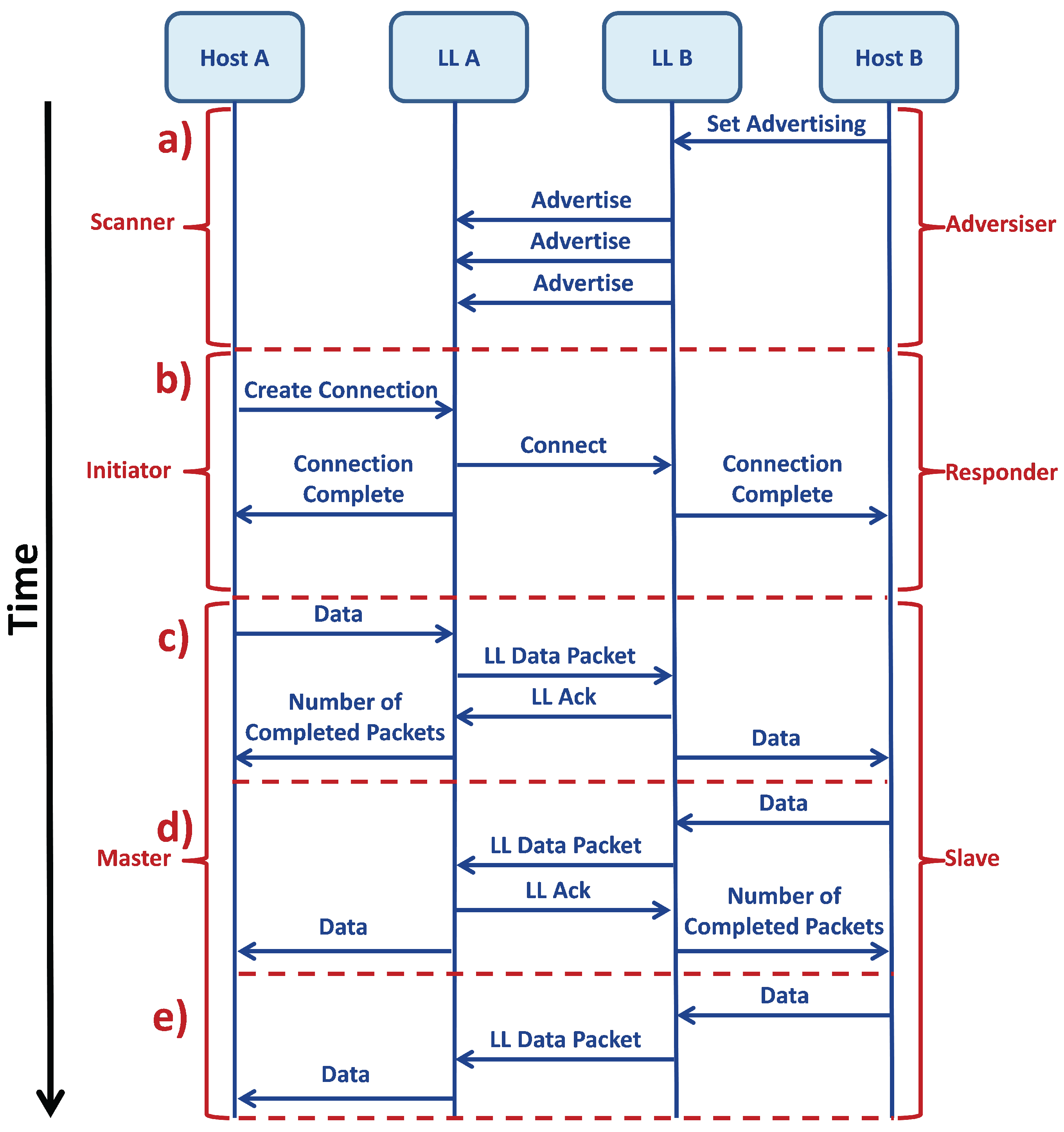
- Broadcaster (Advertiser) periodically sends advertising packets to any device able to receive them.
- Observer (Scanner) continuously scans, at periodic intervals, if there are available advertising packets to receive from a broadcaster.
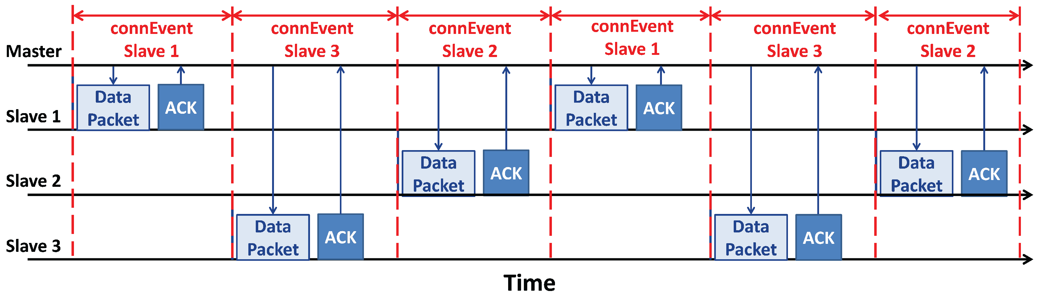
2.2.2. Connections
- The Central (master) scans for connectable advertising packets and initiates the connection. When the connection is active, the central manages all the setting and starts a periodical packet exchanges.
- The Peripheral (slave) periodically sends connectable advertising packets and accepts connections initiated by the master. When the connection is established, it follows the settings exposed by the central and exchanges data with it.
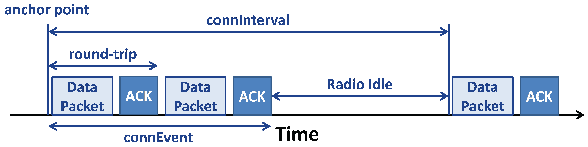
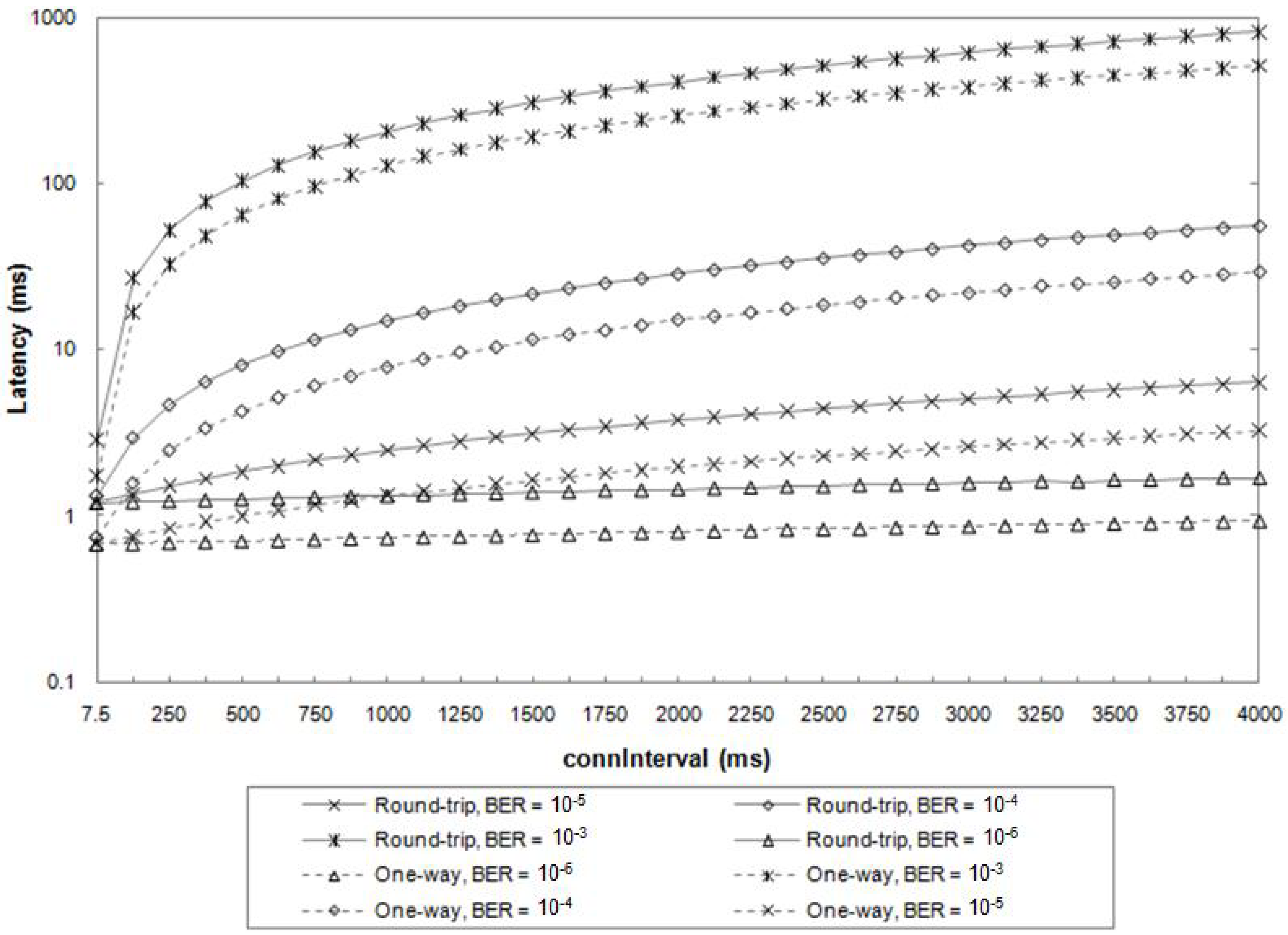
- Connection Interval (connInterval) is the time between the beginning of two consecutive connEvents; in other words, it is the sum of connEvent and Radio Idle. The connInterval shall be a multiple of 1.25 ms in the range of 7.5 ms to 4.0 s.
- Connection Supervision Timeout (connSupervisionTimeout) is the maximum time that can flow without receiving two valid packets, before the connection is lost. The connSupervisionTimeout should be a multiple of 10 in the range of 100 ms to 32,000 ms.
- Connection Slave Latency (connSlaveLatency) is the amount of connEvents that can be skipped without the risk of a disconnection. The value of connSlaveLatency should not cause a connSupervisionTimeout, and it shall be an integer in the range of zero to ((connSupervisionTimeout/(connInterval × 2)) − 1). Moreover, connSlaveLatency shall not be less than 500, and when it is set to zero, the slave device shall listen at every anchor point, without loosing the connection.
- In one-way ATT communication, the slave sends a simple notification in response to a poll from the master. This is typical of the communication through notifiable characteristics.
- In round-trip ATT communication, the master firstly asks for data to the slave, then this one transmits a response. The difference is that both messages, the request and the response, generate an ACK. The interval of time between the beginning of two consecutive data packet, including the ACK, is called .
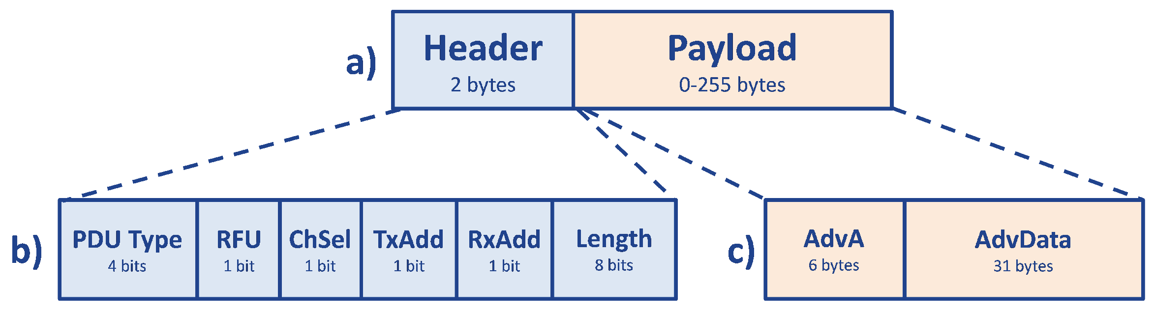
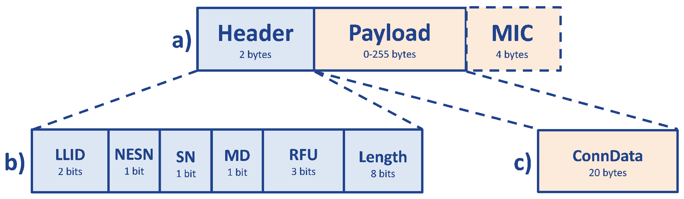
2.3. BLE Packet
- The Preamble (PRE) length depends on the radio data rate, and it is equal to one or two bytes, respectively, if the connection works on LE 1M PHY or on LE 2M PHY, described in Section 2.1.1. It is a very simple sequence of bits used by the receiver to set its automatic gain control and determine the frequency corresponding to the radio data rate itself.
- The Access Address (AA) is the group that includes the four following bytes and identifies the communication on a physical link, and it is used to exclude packets directed to different receivers.
- The Protocol Data Unit (PDU) range is from two to 257 bytes, and its length is strictly dependent on the type of communication used; it is described more in detail below.
- The CRC is a subsection of three bytes, which checks the presence of errors, analyzing the PDU only, which could have been generated during packet transmission. A detailed analysis of error correction techniques, with a specific focus on BLE CRC, has been proposed in [60].
2.4. BLE Network Topology
3. BLE Performance
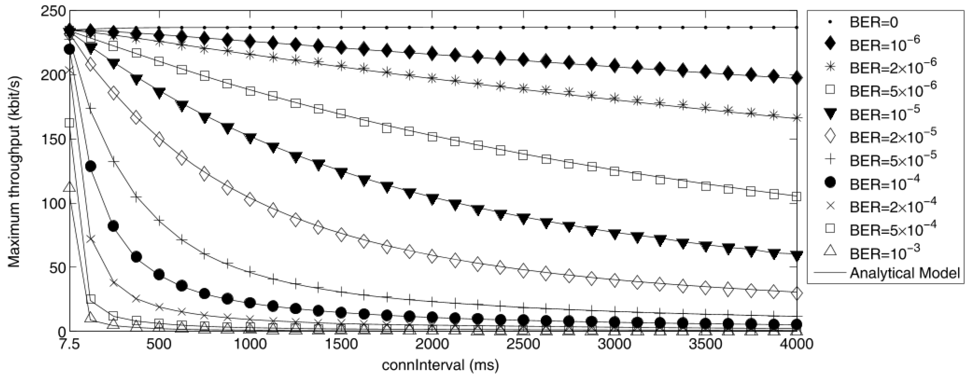
3.1. Throughput
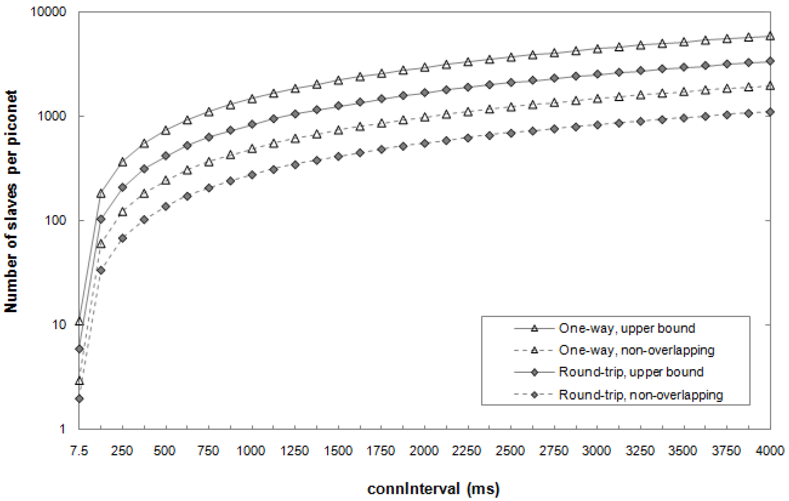
3.2. Piconet Size
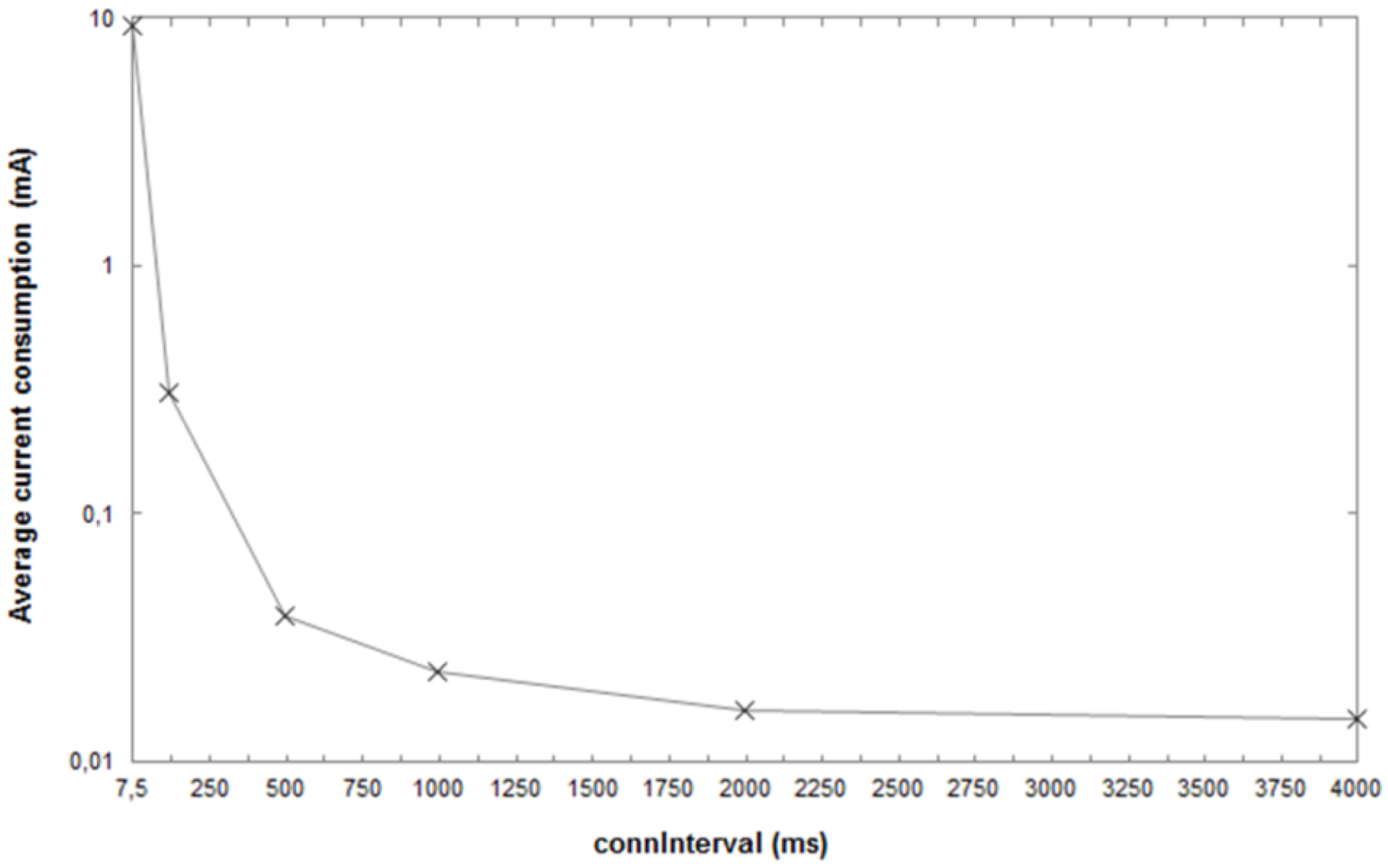
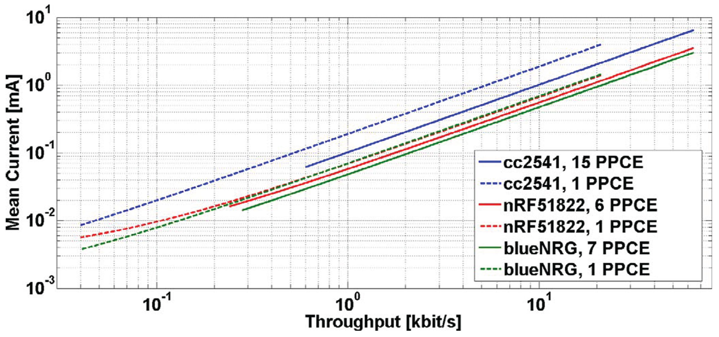
3.3. Power Consumption
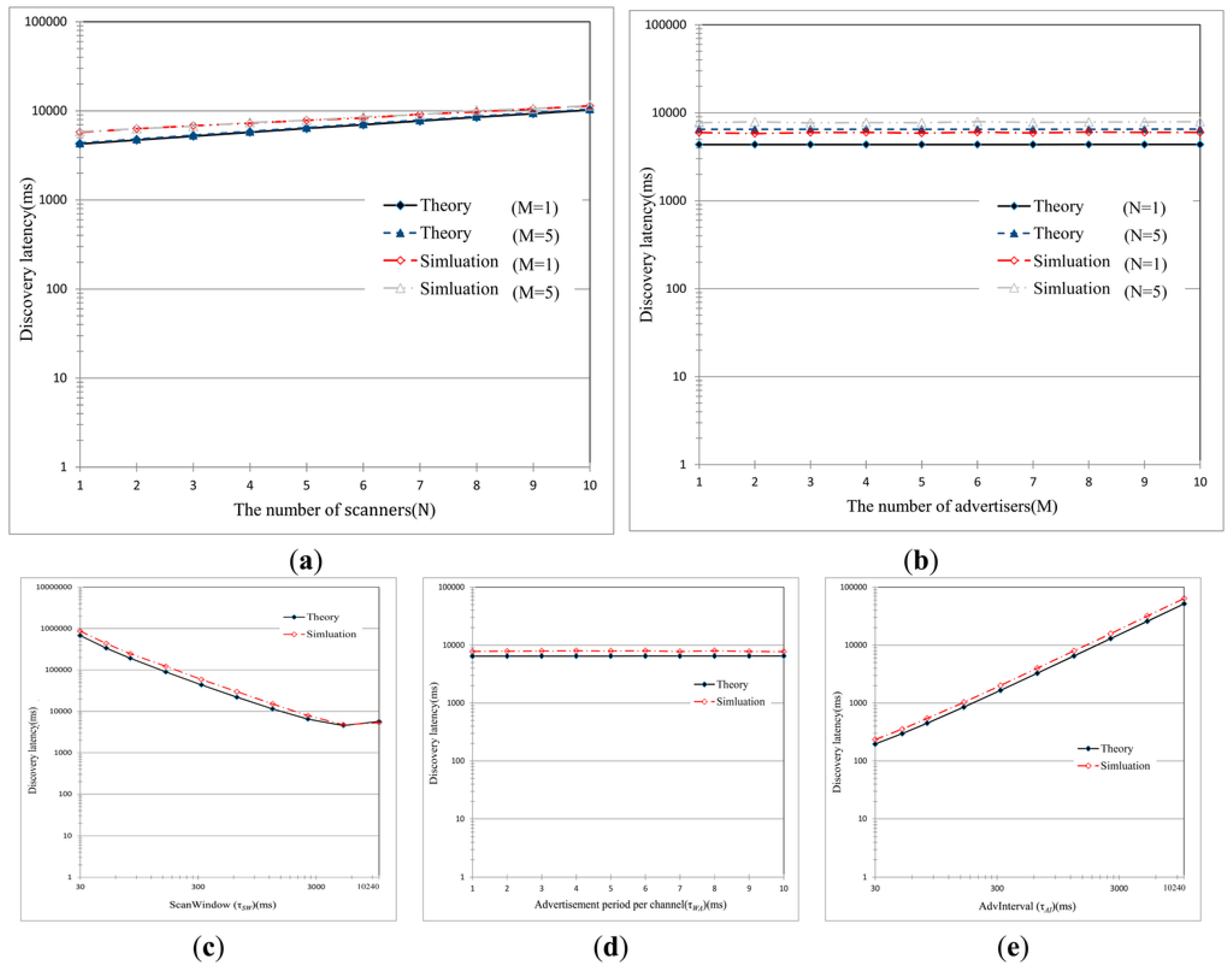
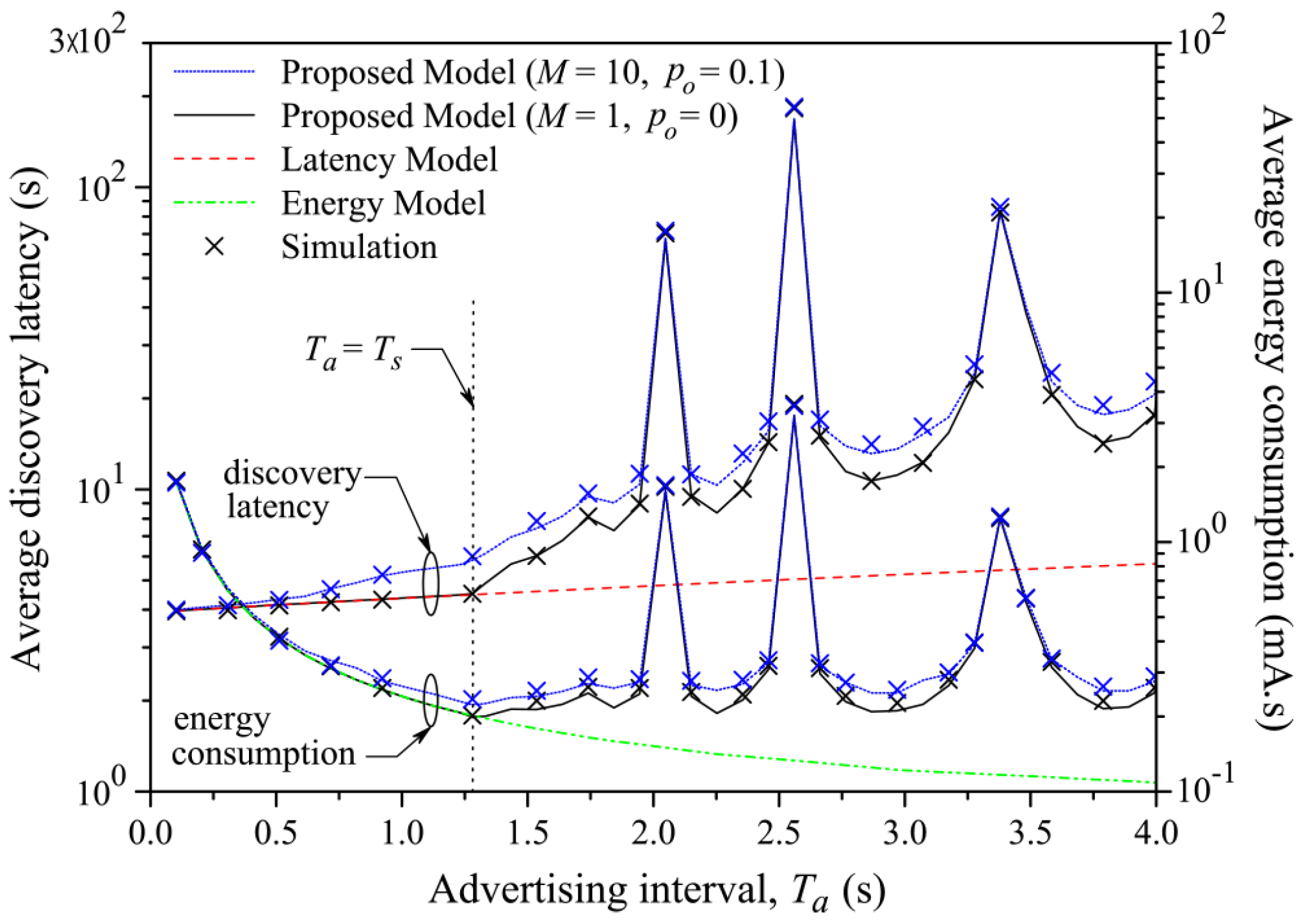
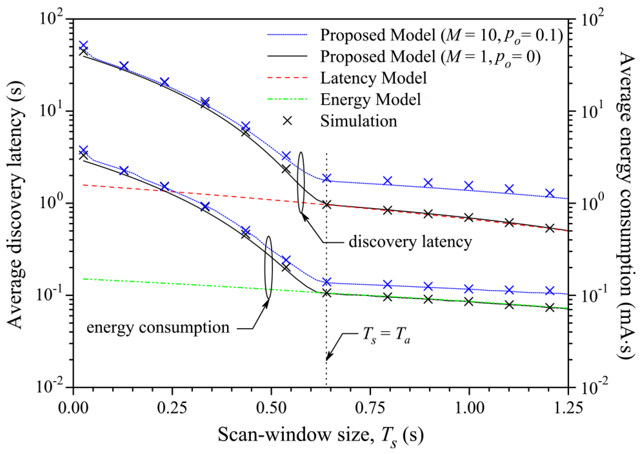
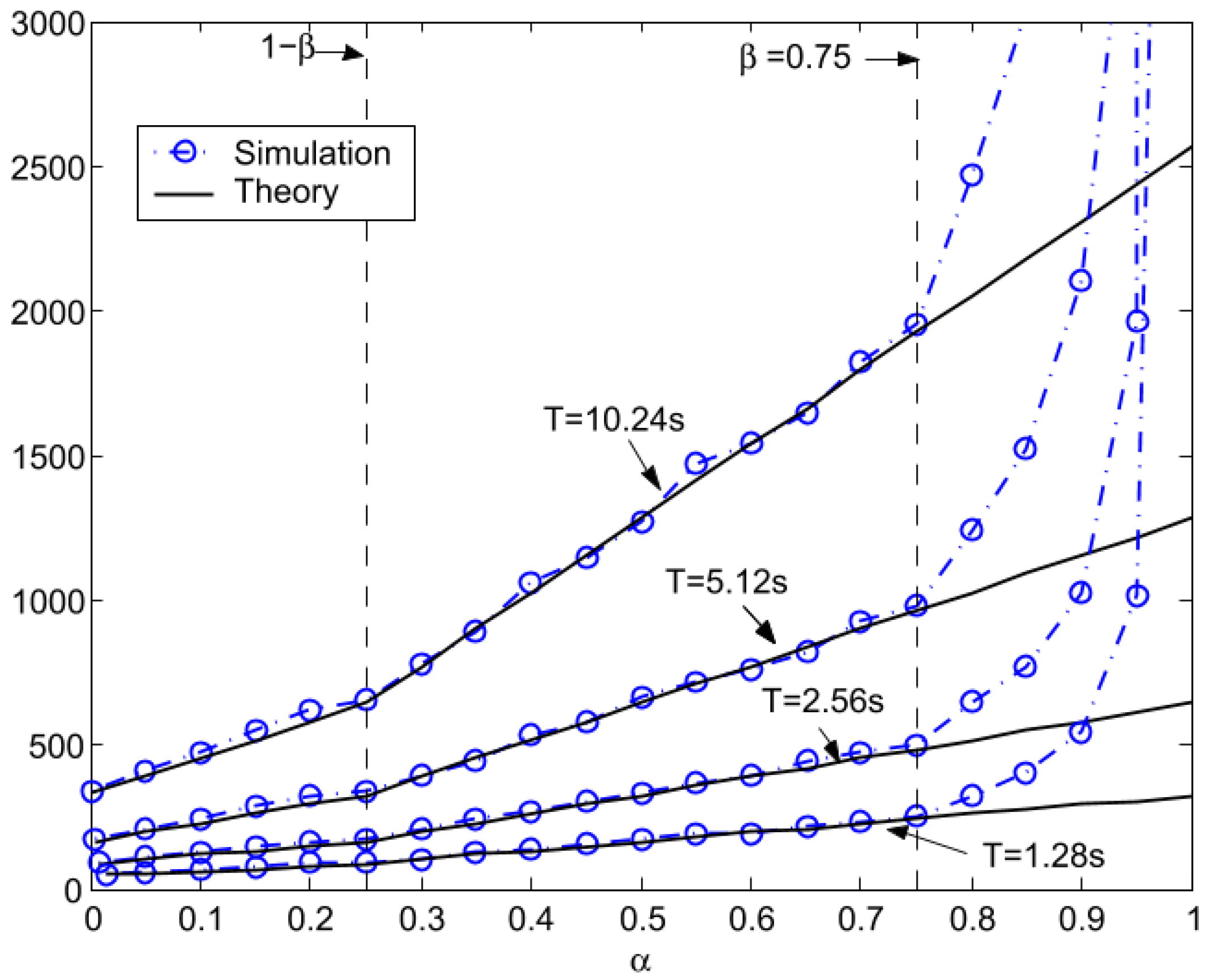
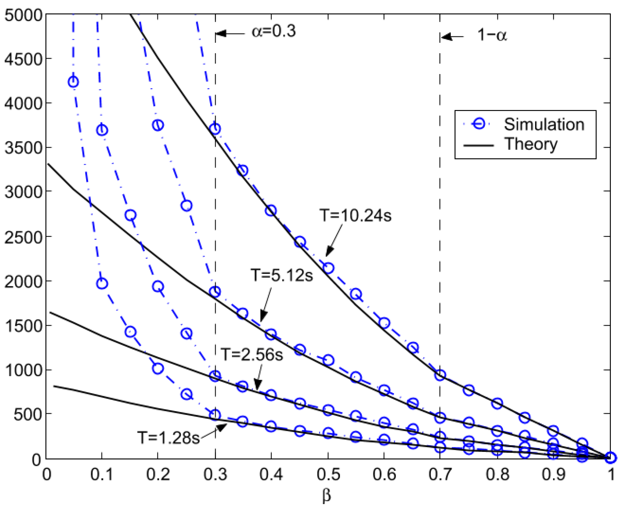
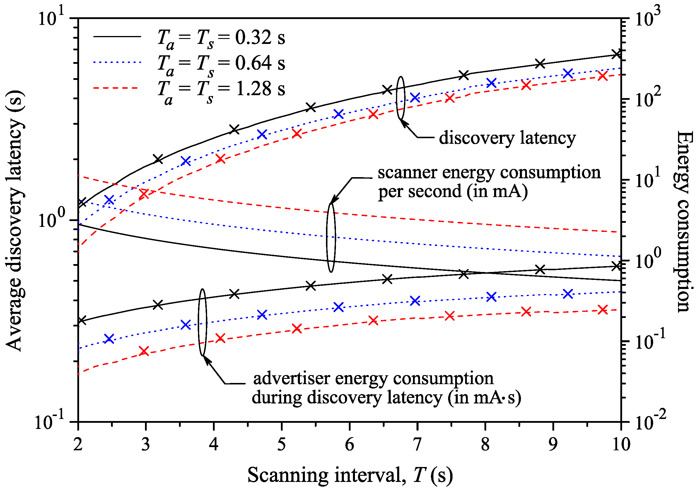
3.4. Latency
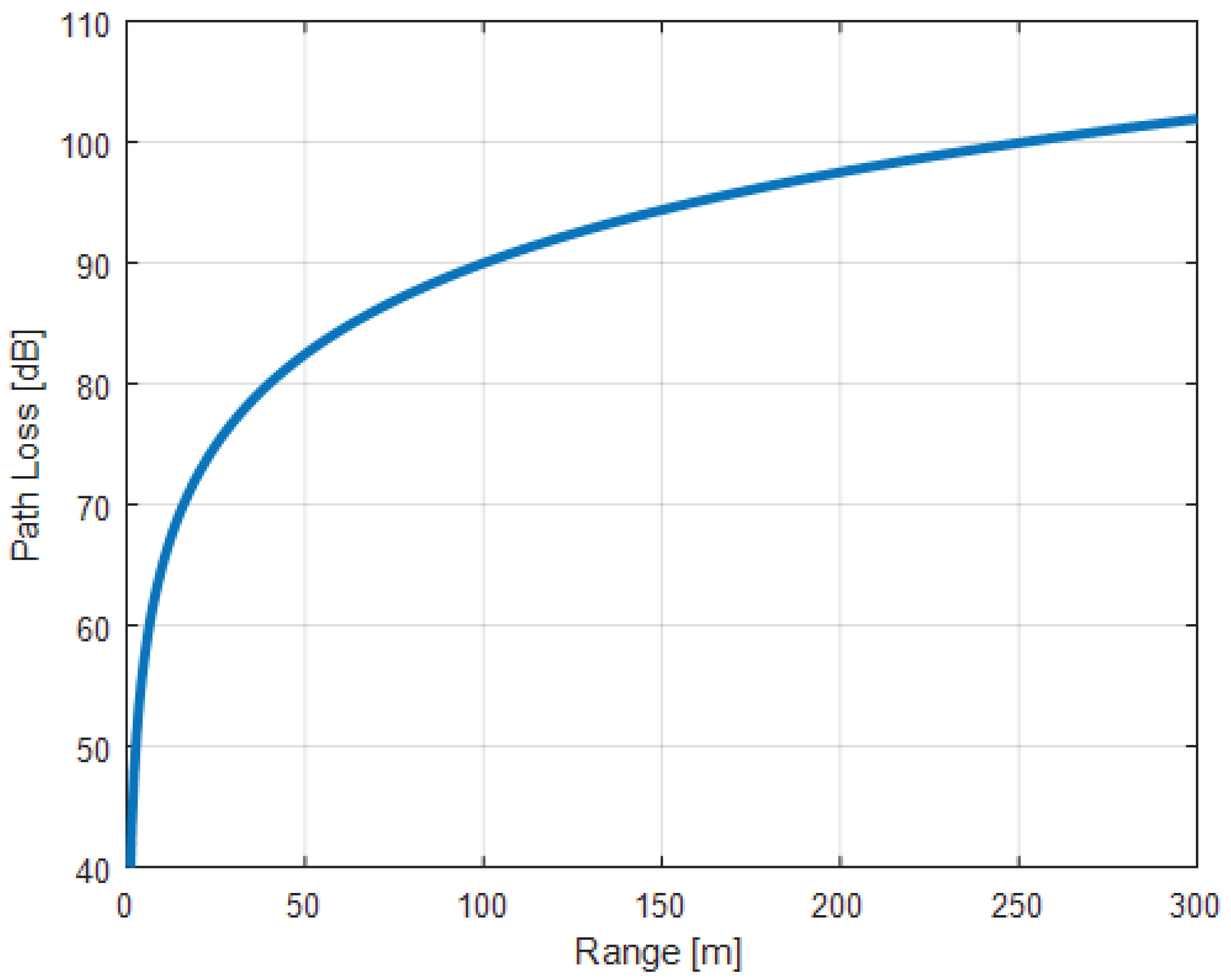
3.5. Range
4. Discussion
Acknowledgments
Conflicts of Interest
Abbreviations
| 6LoWPAN | IPv6 over Low power Wireless Personal Area Networks |
| AA | Access Address |
| ACK | Acknowledgment |
| AdvA | Advertiser’s device Address |
| AdvData | Advertising Data |
| AdvInterval | Advertising Interval |
| AES | Advanced Encryption Standard |
| App | Application Layer |
| ATT | Attribute Protocol |
| BER | Bit Error Rate |
| BLE | Bluetooth Low Energy |
| BR/EDR | Bluetooth Basic Rate/Enhanced Data Rate or Classic Bluetooth |
| ChSel | Channel Selection |
| ConnData | Connection Data |
| ConnEvent | Connection Event |
| ConnInterval | Connection Interval |
| ConnSlaveLatency | Connection Slave Latency |
| ConnSupervisionTimeout | Connection Supervision Timeout |
| CRC | Cyclic Redundancy Check |
| CPU | Central Process Unit |
| FW | Firmware |
| GAP | Generic Access Profile |
| GATT | Generic Attribute Profile |
| HCI | Host Control Interface |
| HW | Hardware |
| IC | Integrated Circuit |
| IETF | Internet Engineering Task Force |
| IoT | Internet of Things |
| IPv6 | Internet Protocol version 6 |
| ISM | Industrial Scientific and Medical |
| L2CAP | Logical Link Control and Adaptation Protocol |
| LE | Low Energy |
| LE 1M PHY | Low Energy 1 Mbps Physical Layer data rate |
| LE 2M PHY | Low Energy 2 Mbps Physical Layer data rate |
| LL | Link Layer |
| LLID | Logical Link Identifier |
| LM | Link Manager |
| MANET | Mobile Ad hoc Networks |
| MD | More Data |
| MIC | Maximum Transmission Unit |
| M-IMU | Magneto-Inertial Measurement Unit |
| MTU | Maximum Transmission Unit |
| NESN | Next Expected Sequence Number |
| OS | Operative Systems |
| PDU | Protocol Data Unit |
| PHY | Physical Layer |
| PPCE | Packets Per Connection Event |
| PRE | Preamble |
| RFCOMM | Radio Frequency Communication |
| RFU | Reserved for Future Use |
| RSSI | Received Signal Strength Indicator |
| RxAdd | Receiver Address |
| ScanInterval | Scanning interval |
| SDP | Service Discovery Protocol |
| SIG | Special Interest Group |
| SMP | Security Manager Protocol |
| SN | Sequence Number |
| SW | Software |
| TxAdd | Transmitter Address |
| UUID | Universal Unique Identifier |
References
- Omre, A.H.; Keeping, S. Bluetooth Low Energy: Wireless Connectivity for Medical Monitoring. J. Diabetes Sci. Technol. 2010, 4, 457–463. [Google Scholar] [PubMed]
- Fekr, A.R.; Radecka, K.; Zilic, Z. Design and Evaluation of an Intelligent Remote Tidal Volume Variability Monitoring System in E-Health Applications. IEEE J. Biomed. Health Inform. 2015, 19, 1532–1548. [Google Scholar] [CrossRef] [PubMed]
- Fafoutis, X.; Vafeas, A.; Janko, B.; Sherratt, R.S.; Pope, J.; Elsts, A.; Mellios, E.; Hilton, G.; Oikonomou, G.; Piechocki, R.; et al. Designing Wearable Sensing Platforms for Healthcare in a Residential Environment. EAI Endorsed Trans. Pervasive Health Technol. 2017, 3. [Google Scholar] [CrossRef]
- Contaldo, M.; Banerjee, B.; Ruffieux, D.; Chabloz, J.; Roux, E.L.; Enz, C.C. A 2.4-GHz BAW-Based Transceiver for Wireless Body Area Networks. IEEE Trans. Biomed. Circuits Syst. 2010, 4, 391–399. [Google Scholar] [CrossRef] [PubMed]
- Park, Y.J.; Cho, H.S. Transmission of ECG data with the patch-type ECG sensor system using Bluetooth Low Energy. In Proceedings of the 2013 International Conference on ICT Convergence (ICTC), Jeju, Korea, 14–16 October 2013; pp. 289–294. [Google Scholar]
- Rachim, V.P.; Chung, W.Y. Wearable Noncontact Armband for Mobile ECG Monitoring System. IEEE Trans. Biomed. Circuits Syst. 2016, 10, 1112–1118. [Google Scholar] [CrossRef] [PubMed]
- Liu, G.; Yang, H.Y. Design and implementation of a Bluetooth 4.0-based heart rate monitor system on iOS platform. In Proceedings of the 2013 International Conference on Communications, Circuits and Systems (ICCCAS), Chengdu, China, 15–17 November 2013; Volume 2, pp. 112–115. [Google Scholar]
- Chan, A.M.; Selvaraj, N.; Ferdosi, N.; Narasimhan, R. Wireless patch sensor for remote monitoring of heart rate, respiration, activity, and falls. In Proceedings of the 2013 35th Annual International Conference of the IEEE Engineering in Medicine and Biology Society (EMBC), Osaka, Japan, 3–7 July 2013; pp. 6115–6118. [Google Scholar]
- Kuwabara, K.; Higuchi, Y.; Ogasawara, T.; Koizumi, H.; Haga, T. Wearable blood flowmeter appcessory with low-power laser Doppler signal processing for daily-life healthcare monitoring. In Proceedings of the 2014 36th Annual International Conference of the IEEE Engineering in Medicine and Biology Society, Chicago, IL, USA, 26–30 August 2014; pp. 6274–6277. [Google Scholar]
- Brunelli, D.; Farella, E.; Giovanelli, D.; Milosevic, B.; Minakov, I. Design Considerations for Wireless Acquisition of Multichannel sEMG Signals in Prosthetic Hand Control. IEEE Sens. J. 2016, 16, 8338–8347. [Google Scholar] [CrossRef]
- Amaro, J.P.; Patrão, S.; Moita, F.; Roseiro, L. Bluetooth low energy profile for MPU9150 IMU data transfers. In Proceedings of the 2017 IEEE 5th Portuguese Meeting on Bioengineering (ENBENG), Coimbra, Portugal, 16–18 February 2017; pp. 1–4. [Google Scholar]
- Lin, J.-R.; Talty, T.; Tonguz, O.K. On the potential of bluetooth low energy technology for vehicular applications. IEEE Commun. Mag. 2015, 53, 267–275. [Google Scholar] [CrossRef]
- Xia, K.; Wang, H.; Wang, N.; Yu, W.; Zhou, T. Design of automobile intelligence control platform based on Bluetooth low energy. In Proceedings of the 2016 IEEE Region 10 Conference (TENCON), Singapore, 22–25 November 2016; pp. 2801–2805. [Google Scholar]
- Gentili, M.; Sannino, R.; Petracca, M. BlueVoice: Voice communications over Bluetooth Low Energy in the Internet of Things scenario. Comput. Commun. 2016, 89–90, 51–59. [Google Scholar] [CrossRef]
- Luan, S.; Gude, D.; Prakash, P.; Warren, S. A paraeducator glove for counting disabled-child behaviors that incorporates a Bluetooth Low Energy wireless link to a smart phone. In Proceedings of the 2014 36th Annual International Conference of the IEEE Engineering in Medicine and Biology Society, Chicago, IL, USA, 26–30 August 2014; pp. 796–799. [Google Scholar]
- Yoon, P.K.; Zihajehzadeh, S.; Kang, B.S.; Park, E.J. Adaptive Kalman filter for indoor localization using Bluetooth Low Energy and inertial measurement unit. In Proceedings of the 2015 37th Annual International Conference of the IEEE Engineering in Medicine and Biology Society (EMBC), Milan, Italy, 25–29 August 2015; pp. 825–828. [Google Scholar]
- Sherratt, R.S.; Janko, B.; Hui, T.; Harwin, W.; Diaz-Sanchez, D. Dictionary memory based software architecture for distributed Bluetooth Low Energy host controllers enabling high coverage in consumer residential healthcare environments. In Proceedings of the 2017 IEEE International Conference on Consumer Electronics (ICCE), Las Vegas, NV, USA, 8–10 January 2017; pp. 406–407. [Google Scholar]
- Collotta, M.; Pau, G. A Novel Energy Management Approach for Smart Homes Using Bluetooth Low Energy. IEEE J. Sel. Areas Commun. 2015, 33, 2988–2996. [Google Scholar] [CrossRef]
- Collotta, M.; Pau, G. A Solution Based on Bluetooth Low Energy for Smart Home Energy Management. Energies 2015, 8, 11916–11938. [Google Scholar] [CrossRef]
- Collotta, M.; Pau, G. An Innovative Approach for Forecasting of Energy Requirements to Improve a Smart Home Management System Based on BLE. IEEE Trans. Green Commun. Netw. 2017, 1, 112–120. [Google Scholar] [CrossRef]
- Tian, J.; Liu, J.; Liang, S.; Ning, Y.; Li, H.; Zhao, G. Wireless transmission system for motion sensing game controller based on low power Bluetooth technology. In Proceedings of the 2016 IEEE 13th International Conference on Signal Processing (ICSP), Chengdu, China, 6–10 November 2016; pp. 1318–1322. [Google Scholar]
- Karani, R.; Dhote, S.; Khanduri, N.; Srinivasan, A.; Sawant, R.; Gore, G.; Joshi, J. Implementation and design issues for using Bluetooth low energy in passive keyless entry systems. In Proceedings of the 2016 IEEE Annual India Conference (INDICON), Bangalore, India, 16–18 December 2016; pp. 1–6. [Google Scholar]
- Koodtalang, W.; Sangsuwan, T. Improving motorcycle anti-theft system with the use of Bluetooth Low Energy 4.0. In Proceedings of the 2016 International Symposium on Intelligent Signal Processing and Communication Systems (ISPACS), Phuket, Thailand, 24–27 October 2016; pp. 1–5. [Google Scholar]
- Basalamah, A. Sensing the Crowds Using Bluetooth Low Energy Tags. IEEE Access 2016, 4, 4225–4233. [Google Scholar] [CrossRef]
- Alletto, S.; Cucchiara, R.; Fiore, G.D.; Mainetti, L.; Mighali, V.; Patrono, L.; Serra, G. An Indoor Location-Aware System for an IoT-Based Smart Museum. IEEE Int. Things J. 2016, 3, 244–253. [Google Scholar] [CrossRef]
- Zou, H.; Jiang, H.; Luo, Y.; Zhu, J.; Lu, X.; Xie, L. BlueDetect: An iBeacon-Enabled Scheme for Accurate and Energy-Efficient Indoor-Outdoor Detection and Seamless Location-Based Service. Sensors 2016, 16, 268. [Google Scholar] [CrossRef] [PubMed]
- Lin, X.Y.; Ho, T.W.; Fang, C.C.; Yen, Z.S.; Yang, B.J.; Lai, F. A mobile indoor positioning system based on iBeacon technology. In Proceedings of the 2015 37th Annual International Conference of the IEEE Engineering in Medicine and Biology Society (EMBC), Milan, Italy, 25–29 August 2015; pp. 4970–4973. [Google Scholar]
- Mokhtari, G.; Zhang, Q.; Karunanithi, M. Modeling of human movement monitoring using Bluetooth Low Energy technology. Conf. Proc. IEEE Eng. Med. Biol. Soc. 2015, 2015, 5066–5069. [Google Scholar] [PubMed]
- Ozer, A.; John, E. Improving the Accuracy of Bluetooth Low Energy Indoor Positioning System Using Kalman Filtering. In Proceedings of the 2016 International Conference on Computational Science and Computational Intelligence (CSCI), Las Vegas, NV, USA, 15–17 December 2016; pp. 180–185. [Google Scholar]
- Peng, Y.; Fan, W.; Dong, X.; Zhang, X. An Iterative Weighted KNN (IW-KNN) Based Indoor Localization Method in Bluetooth Low Energy (BLE) Environment. In Proceedings of the 2016 International IEEE Conferences on Ubiquitous Intelligence Computing, Advanced and Trusted Computing, Scalable Computing and Communications, Cloud and Big Data Computing, Internet of People, and Smart World Congress (UIC/ATC/ScalCom/CBDCom/IoP/SmartWorld), Toulouse, France, 18–21 July 2016; pp. 794–800. [Google Scholar]
- Viswanathan, S.; Srinivasan, S. Improved path loss prediction model for short range indoor positioning using bluetooth low energy. In Proceedings of the 2015 IEEE SENSORS, Busan, Korea, 1–4 November 2015; pp. 1–4. [Google Scholar]
- Kotanen, A.; Hannikainen, M.; Leppakoski, H.; Hamalainen, T.D. Experiments on local positioning with Bluetooth. In Proceedings of the International Conference on Information Technology: Coding and Computing, Las Vegas, NV, USA, 28–30 April 2003; pp. 297–303. [Google Scholar]
- Bae, H.; Oh, J.; Lee, K.; Oh, J.H. Low-cost indoor positioning system using BLE (bluetooth low energy) based sensor fusion with constrained extended Kalman Filter. In Proceedings of the 2016 IEEE International Conference on Robotics and Biomimetics (ROBIO), Qingdao, China, 3–7 December 2016; pp. 939–945. [Google Scholar]
- Lee, C.H. Location-Aware Speakers for the Virtual Reality Environments. IEEE Access 2017, 5, 2636–2640. [Google Scholar] [CrossRef]
- Apoorv, R.; Mathur, P. Smart attendance management using Bluetooth Low Energy and Android. In Proceedings of the 2016 IEEE Region 10 Conference (TENCON), Singapore, 22–25 November 2016; pp. 1048–1052. [Google Scholar]
- Filippoupolitis, A.; Oliff, W.; Loukas, G. Bluetooth Low Energy Based Occupancy Detection for Emergency Management. In Proceedings of the 2016 15th International Conference on Ubiquitous Computing and Communications and 2016 International Symposium on Cyberspace and Security (IUCC-CSS), Granada, Spain, 14–16 December 2016; pp. 31–38. [Google Scholar]
- Kumar, B.G.A.; Bhagyalakshmi, K.C.; Lavanya, K.; Gowranga, K.H. A Bluetooth low energy based beacon system for smart short range surveillance. In Proceedings of the 2016 IEEE International Conference on Recent Trends in Electronics, Information Communication Technology (RTEICT), Bangalore, India, 20–21 May 2016; pp. 1181–1184. [Google Scholar]
- Varela, P.M.; Ohtsuki, T.O. Discovering Co-Located Walking Groups of People Using iBeacon Technology. IEEE Access 2016, 4, 6591–6601. [Google Scholar] [CrossRef]
- Palattella, M.R.; Dohler, M.; Grieco, A.; Rizzo, G.; Torsner, J.; Engel, T.; Ladid, L. Internet of Things in the 5G Era: Enablers, Architecture, and Business Models. IEEE J. Sel. Areas Commun. 2016, 34, 510–527. [Google Scholar] [CrossRef]
- Wang, H.; Xi, M.; Liu, J.; Chen, C. Transmitting IPv6 packets over Bluetooth low energy based on BlueZ. In Proceedings of the 2013 15th International Conference on Advanced Communication Technology (ICACT), PyeongChang, Korea, 27–30 January 2013; pp. 72–77. [Google Scholar]
- Kushalnagar, N.; Montenegro, G.; Schumacher, C. IPv6 over Low-Power Wireless Personal Area Networks (6LoWPANs): Overview, Assumptions, Problem Statement, and Goals, August 2007. Available online: https://tools.ietf.org/html/rfc4919 (accessed on 12 December 2017).
- Raza, S.; Misra, P.; He, Z.; Voigt, T. Bluetooth smart: An enabling technology for the Internet of Things. In Proceedings of the 2015 IEEE 11th International Conference on Wireless and Mobile Computing, Networking and Communications (WiMob), Abu Dhabi, United Arab Emirates, 19–21 October 2015; pp. 155–162. [Google Scholar]
- Tabish, R.; Mnaouer, A.B.; Touati, F.; Ghaleb, A.M. A comparative analysis of BLE and 6LoWPAN for U-HealthCare applications. In Proceedings of the 2013 7th IEEE GCC Conference and Exhibition (GCC), Doha, Qatar, 17–20 November 2013; pp. 286–291. [Google Scholar]
- Isomaki, M.; Nieminen, J.; Gomez, C.; Shelby, Z.; Savolainen, T.; Patil, B. Transmission of IPv6 Packets over Bluetooth Low Energy, February 2013. Available online: https://tools.ietf.org/html/draft-ietf-6lowpan-btle-12 (accessed on 12 December 2017).
- STMicroelectronics. STM32 ODE function pack for connecting 6LoWPAN IoT nodes to smarphones via BLE interface. In Data Brief FP-NET-6LPBLE1 2016; STMicroelectronics: Ginevra, Svizzera, 2016; Available online: https://www.st.com/ (accessed on 12 December 2017).
- Pau, G.; Collotta, M.; Maniscalco, V. Bluetooth 5 Energy Management through a Fuzzy-PSO Solution for Mobile Devices of Internet of Things. Energies 2017, 10, 992. [Google Scholar]
- Marco, P.D.; Skillermark, P.; Larmo, A.; Arvidson, P.; Chirikov, R. Performance Evaluation of the Data Transfer Modes in Bluetooth 5. IEEE Commun. Stand. Mag. 2017, 1, 92–97. [Google Scholar] [CrossRef]
- Townsend, K.; Cufi, C.; Akiba; Davidson, R. Protocol Basics. In Getting Started with Bluetooth Low Energy: Tools and Techniques for Low-Power Networking; Sawyer, B., Loukides, M., Eds.; O’Reilly Media, Inc.: Sebastopol, CA, USA, 2014; pp. 15–34. [Google Scholar]
- Heydon, K. Architecture. In Bluetooth Low Energy—The Developer’s Handbook; Goodwin, B., Ed.; Prantice Hall-Pearson Education, Inc.: Upper Saddle River, NJ, USA, 2012; pp. 40–51. [Google Scholar]
- Gomez, C.; Oller, J.; Paradells, J. Overview and Evaluation of Bluetooth Low Energy: An Emerging Low-Power Wireless Technology. Sensors 2012, 12, 11734–11753. [Google Scholar] [CrossRef]
- Gupta, N.K. Inside Bluetooth Low Energy, 2nd ed.; Google-Books-ID: 3nCuDgAAQBAJ; Artech House; SNorwood, MA, USA, 2016. [Google Scholar]
- Townsend, K.; Cufi, C.; Wang, C.; Davidson, R. Introduction. In Getting Started with Bluetooth Low Energy: Tools and Techniques for Low-Power Networking; Sawyer, B., Loukides, M., Eds.; O’Reilly Media, Inc.: Sebastopol, CA, USA, 2014; pp. 1–14. [Google Scholar]
- BluetoothSIG. Vol 6: Core System Package [Low Energy Specification], Part A: Physical Layer Specification. In Specification of the Bluetooth® System, Covered Core Package Version: 5.0; The Bluetooth Special Interest Group: Kirkland, WA, USA, 2016; pp. 2532–2546. Available online: https://www.bluetooth.org/ (accessed on 12 December 2017).
- Heydon, K. The Host/Controller Interface. In Bluetooth Low Energy—The Developer’s Handbook; Goodwin, B., Ed.; Prantice Hall- Pearson Education, Inc.: Upper Saddle River, NJ, USA, 2012; pp. 131–163. [Google Scholar]
- Heydon, K. The Physical Layer. In Bluetooth Low Energy—The Developer’s Handbook; Goodwin, B., Ed.; Prantice Hall-Pearson Education, Inc.: Upper Saddle River, NJ, USA, 2012; pp. 59–69. [Google Scholar]
- Heydon, K. Basic Concepts. In Bluetooth Low Energy—The Developer’s Handbook; Goodwin, B., Ed.; Prantice Hall-Pearson Education, Inc.: Upper Saddle River, NJ, USA, 2012; pp. 28–39. [Google Scholar]
- Townsend, K.; Cufi, C.; Wang, C.; Davidson, R. GAP (Advertising and Connections). In Getting Started with Bluetooth Low Energy: Tools and Techniques for Low-Power Networking; Sawyer, B., Loukides, M., Eds.; O’Reilly Media, Inc.: Sebastopol, CA, USA, 2014; pp. 35–50. [Google Scholar]
- BluetoothSIG. Vol 6: Core System Package [Low Energy Specification], Part B: Link Layer Specification. In Specification of the Bluetooth® System, Covered Core Package Version: 5.0; The Bluetooth Special Interest Group: Kirkland, WA, USA, 2016; pp. 2547–2694. Available online: https://www.bluetooth.org/ (accessed on 12 December 2017).
- BluetoothSIG. Vol 1: Architecture & Terminology Overview, Part A: Architecture. In Specification of the Bluetooth® System, Covered Core Package Version: 5.0; The Bluetooth Special Interest Group: Kirkland, WA, USA, 2016; pp. 161–264. Available online: https://www.bluetooth.org/ (accessed on 12 December 2017).
- Tsimbalo, E.; Fafoutis, X.; Piechocki, R.J. CRC Error Correction in IoT Applications. IEEE Trans. Ind. Inform. 2017, 13, 361–369. [Google Scholar] [CrossRef]
- Harris, A.F., III; Khanna, V.; Tuncay, G.; Want, R.; Kravets, R. Bluetooth Low Energy in Dense IoT Environments. IEEE Commun. Mag. 2016, 54, 30–36. [Google Scholar] [CrossRef]
- BluetoothSIG. Vol 3: Core System Package [Host Volume], Part G: Generic Attribute Profile. In Specification of the Bluetooth® System, Covered Core Package Version: 5.0; The Bluetooth Special Interest Group: Kirkland, WA, USA, 2016; pp. 2217–2288. Available online: https://www.bluetooth.org/ (accessed on 12 December 2017).
- León, J.; Dueñas, A.; Iano, Y.; Makluf, C.A.; Kemper, G. A Bluetooth Low Energy mesh network auto-configuring Proactive Source Routing protocol. In Proceedings of the 2017 IEEE International Conference on Consumer Electronics (ICCE), Las Vegas, NV, USA, 8–10 January 2017; pp. 348–349. [Google Scholar]
- Darroudi, S.M.; Gomez, C. Bluetooth Low Energy Mesh Networks: A Survey. Sensors 2017, 17, 1467. [Google Scholar] [CrossRef] [PubMed]
- Gomez, C.; Demirkol, I.; Paradells, J. Modeling the Maximum Throughput of Bluetooth Low Energy in an Error-Prone Link. IEEE Commun. Lett. 2011, 15, 1187–1189. [Google Scholar] [CrossRef]
- Apple. Bluetooth Accessory Design Guidelines for Apple Products—Release R7 2013. Apple Developer-Apple Inc. Available online: https://developer.apple.com/hardwaredrivers/{BluetoothDesignGuidelines}.pdf (accessed on 12 December 2017).
- Nordic Semiconductor. nRF51822: Multiprotocol Bluetooth Low Energy and 204 GHz Proprietary System-On-Chip. In nRF51822 Product Brief Version 2.5 2013; Nordic Semiconductor: Trondheim, Oslo, Norway, 2013; Available online: infocenter.nordicsemi.com/ (accessed on 12 December 2017).
- STMicroelectronics. BlueNRG Current Consumption Estimation Tool. In STSW-BNRG001 2016; STMicroelectronics: Ginevra, Svizzera, 2016; Available online: https://www.st.com/ (accessed on 12 December 2017).
- STMicroelectronics. Upgradable Bluetooth® Low Energy Network Processor. In Datasheet-Production Data BlueNRG-MS 2016; STMicroelectronics: Ginevra, Svizzera, 2016; Available online: https://www.st.com/ (accessed on 12 December 2017).
- Tei, R.; Yamazawa, H.; Shimizu, T. BLE power consumption estimation and its applications to smart manufacturing. In Proceedings of the 2015 54th Annual Conference of the Society of Instrument and Control Engineers of Japan (SICE), Hangzhou, China, 28–30 July 2015; pp. 148–153. [Google Scholar]
- STMicroelectronics. BlueNRG-MS Bluetooth® LE Stack Application Command Interface (ACI). In UM1865 User Manual 2017; STMicroelectronics: Ginevra, Svizzera, 2016; Available online: https://www.st.com/ (accessed on 9 September 2016).
- Texas Instruments. BLE-Stack User’s Guide for Bluetooth 4.2 (V. 3.01.00.05) 2017; Texas Instruments: Dallas, TX, USA, 2010; Available online: https://www.ti.com/ (accessed on 29 August 2017).
- Rheinländer, C.C.; Wehn, N. Precise synchronization time stamp generation for Bluetooth low energy. In Proceedings of the 2016 IEEE SENSORS, Orlando, FL, USA, 30 October–3 November 2016; pp. 1–3. [Google Scholar]
- Habbal, M. Bluetooth low energy–assessment within a competing wireless world. In Proceedings of the Wireless Congress 2012-Systems & Applications, Munich, Germany, 14–15 November 2012. [Google Scholar]
- Want, R.; Schilit, B.; Laskowski, D. Bluetooth LE Finds Its Niche. IEEE Pervasive Comput. 2013, 12, 12–16. [Google Scholar] [CrossRef]
- Liu, J.; Chen, C.; Ma, Y.; Xu, Y. Energy Analysis of Device Discovery for Bluetooth Low Energy. In Proceedings of the 2013 IEEE 78th Vehicular Technology Conference (VTC Fall), Las Vegas, NV, USA, 2–5 September 2013; pp. 1–5. [Google Scholar]
- Texas Instruments. CC2541: 2.4-GHz Bluetooth® Low Energy and Proprietary System-On-Chip. In SWRS110D 2013; Texas Instruments: Dallas, TX, USA, 2010; Available online: https://www.ti.com/ (accessed on 9 September 2016).
- Jeon, W.S.; Dwijaksara, M.H.; Jeong, D.G. Performance Analysis of Neighbor Discovery Process in Bluetooth Low-Energy Networks. IEEE Trans. Veh. Technol. 2017, 66, 1865–1871. [Google Scholar] [CrossRef]
- Liu, J.; Chen, C.; Ma, Y. Modeling Neighbor Discovery in Bluetooth Low Energy Networks. IEEE Commun. Lett. 2012, 16, 1439–1441. [Google Scholar] [CrossRef]
- Kim, J.; Han, K. Backoff scheme for crowded Bluetooth low energy networks. IET Commun. 2017, 11, 548–557. [Google Scholar] [CrossRef]
- Kamath, S.; Lindh, J. Measuring bluetooth low energy power consumption. In Application Note AN092 2010; Texas Instruments: Dallas, TX, USA, 2010; Available online: https://www.ti.com/ (accessed on 9 September 2016).
- NXP Semiconductors. MKW40Z Power Consumption Analysis. In Application Note AN5272 2016; NXP Semiconductor: Eindhoven, The Netherlands; Available online: https://www.nxp.com/ (accessed on 30 August 2017).
- Texas Instruments. CC2540: 2.4-GHz Bluetooth® Low Energy and Proprietary System-On-Chip. In SWRS084F 2013; Texas Instruments: Dallas, TX, USA, 2010; Available online: https://www.ti.com/ (accessed on 9 September 2016).
- Feng, Z.; Mo, L.; Li, M. Analysis of low energy consumption wireless sensor with BLE. In Proceedings of the 2015 IEEE SENSORS, Busan, Korea, 1–4 November 2015; pp. 1–4. [Google Scholar]
- Giovanelli, D.; Milosevic, B.; Farella, E. Bluetooth Low Energy for data streaming: Application-level analysis and recommendation. In Proceedings of the 2015 6th International Workshop on Advances in Sensors and Interfaces (IWASI), Gallipoli, Italy, 18–19 June 2015; pp. 216–221. [Google Scholar]
- STMicroelectronics. BlueNRG-Upgradable Bluetooth® Low Energy network processor. In DocID025108-Datasheet 2016; STMicroelectronics: Ginevra, Svizzera, 2016; Available online: https://www.st.com/ (accessed on 31 August 2017).
- Aguilar, S.; Vidal, R.; Gomez, C. Opportunistic Sensor Data Collection with Bluetooth Low Energy. Sensors 2017, 17, 159. [Google Scholar] [CrossRef] [PubMed]
- Cho, K.; Park, W.; Hong, M.; Park, G.; Cho, W.; Seo, J.; Han, K. Analysis of Latency Performance of Bluetooth Low Energy (BLE) Networks. Sensors 2014, 15, 59–78. [Google Scholar] [CrossRef] [PubMed]
- Cho, K.; Jung, C.; Kim, J.; Yoon, Y.; Han, K. Modeling and analysis of performance based on Bluetooth Low Energy. In Proceedings of the 2015 7th IEEE Latin-American Conference on Communications (LATINCOM), Arequipa, Peru, 4–6 November 2015; pp. 1–6. [Google Scholar]
- Liu, J.; Chen, C.; Ma, Y. Modeling and performance analysis of device discovery in Bluetooth Low Energy networks. In Proceedings of the 2012 IEEE Global Communications Conference (GLOBECOM), Anaheim, CA, USA, 3–7 Decemer 2012; pp. 1538–1543. [Google Scholar]
- Contreras, D.; Castro, M.; de la Torre, D.S. Performance evaluation of bluetooth low energy in indoor positioning systems. Trans. Emerg. Telecommun. Technol. 2017, 28. [Google Scholar] [CrossRef]
- Kajikawa, N.; Minami, Y.; Kohno, E.; Kakuda, Y. On Availability and Energy Consumption of the Fast Connection Establishment Method by Using Bluetooth Classic and Bluetooth Low Energy. In Proceedings of the 2016 Fourth International Symposium on Computing and Networking (CANDAR), Hiroshima, Japan, 22–25 November 2016; pp. 286–290. [Google Scholar]
- Buckley, J.; Aherne, K.; O’Flynn, B.; Barton, J.; Murphy, A.; O’Mathuna, C. Antenna performance measurements using wireless sensor networks. In Proceedings of the 56th Electronic Components and Technology Conference 2006, San Diego, CA, USA, 30 May–2 June 2006; p. 6. [Google Scholar]
- Pattnayak, T.; Thanikachalam, G. Antenna Design and RF Layout Guidelines. In Cypress Semiconductor AN91445; Cypress Semiconductor: San Jose, CA, USA, 2015; Available online: http://www.cypress.com/ (accessed on 30 August 2017).


| Key-Parameters | Description | Characteristic Addressed |
|---|---|---|
| connEvent Section 2.2.2 | The time in which two devices exchange packets | Throughput Section 3.1, Latency Section 3.4, Power consumption Section 3.3, Piconet size Section 3.2 |
| connInterval Section 2.2.2 | The time between two consecutive connEvents | Throughput Section 3.1, Latency Section 3.4, Power consumption Section 3.3, Piconet size Section 3.2 |
| Radio Idle Section 2.2.2 | The period between two consecutive connEvents, when the communication is off | Throughput Section 3.1, Latency Section 3.4, Power consumption Section 3.3, Piconet size Section 3.2 |
| connSlaveLatency Section 2.2.2 | Amount of connEvents which can be skipped avoiding the risk of disconnections | Piconet size Section 3.2, Latency Section 3.4 |
| advInterval Section 2.2.1 | The rate at which advertising packets are sent | Power consumption Section 3.3, Latency Section 3.4 |
| scanInterval Section 2.2.1 | The rate at which the scanner’s radio turns on | Power consumption Section 3.3, Latency Section 3.4 |
| scanWindow Section 2.2.1 | The amount of time the radio keeps on scanning | Latency Section 3.4 |
| round-trip Section 2.2.2 | The time to send a data packet and an ACK. | Throughput Section 3.1, Latency Section 3.4 |
| one-way Section 2.2.2 | The time to send a packet in notification mode | Throughput Section 3.1, Latency Section 3.4 |
| payload Section 2.3 | Number of bytes per each data packet, that is 20 bytes | Throughput Section 3.1 |
| piconet Section 2.4 | A basic BLE network, composed by a master and a slave | Piconet size Section 3.2 |
| scatternet Section 2.4 | A network where a device performs master and slave simultaneously. | Piconet size Section 3.2 |
© 2017 by the authors. Licensee MDPI, Basel, Switzerland. This article is an open access article distributed under the terms and conditions of the Creative Commons Attribution (CC BY) license (http://creativecommons.org/licenses/by/4.0/).
Share and Cite
Tosi, J.; Taffoni, F.; Santacatterina, M.; Sannino, R.; Formica, D. Performance Evaluation of Bluetooth Low Energy: A Systematic Review. Sensors 2017, 17, 2898. https://doi.org/10.3390/s17122898
Tosi J, Taffoni F, Santacatterina M, Sannino R, Formica D. Performance Evaluation of Bluetooth Low Energy: A Systematic Review. Sensors. 2017; 17(12):2898. https://doi.org/10.3390/s17122898
Chicago/Turabian StyleTosi, Jacopo, Fabrizio Taffoni, Marco Santacatterina, Roberto Sannino, and Domenico Formica. 2017. "Performance Evaluation of Bluetooth Low Energy: A Systematic Review" Sensors 17, no. 12: 2898. https://doi.org/10.3390/s17122898
APA StyleTosi, J., Taffoni, F., Santacatterina, M., Sannino, R., & Formica, D. (2017). Performance Evaluation of Bluetooth Low Energy: A Systematic Review. Sensors, 17(12), 2898. https://doi.org/10.3390/s17122898