Author Contributions
Conceptualization, A.Q.-C. and H.B.; methodology, H.B.; software, S.J. and A.T.; validation, H.B. and A.I.; formal analysis, H.B. and A.I.; investigation, H.B.; resources, S.J.; data curation, A.T.; writing—original draft preparation, H.B.; writing—review and editing, A.Q.-C., A.I. and H.B.; visualization, H.B.; supervision, A.Q.-C. and S.J.; project administration, S.J. All authors have read and agreed to the published version of the manuscript.
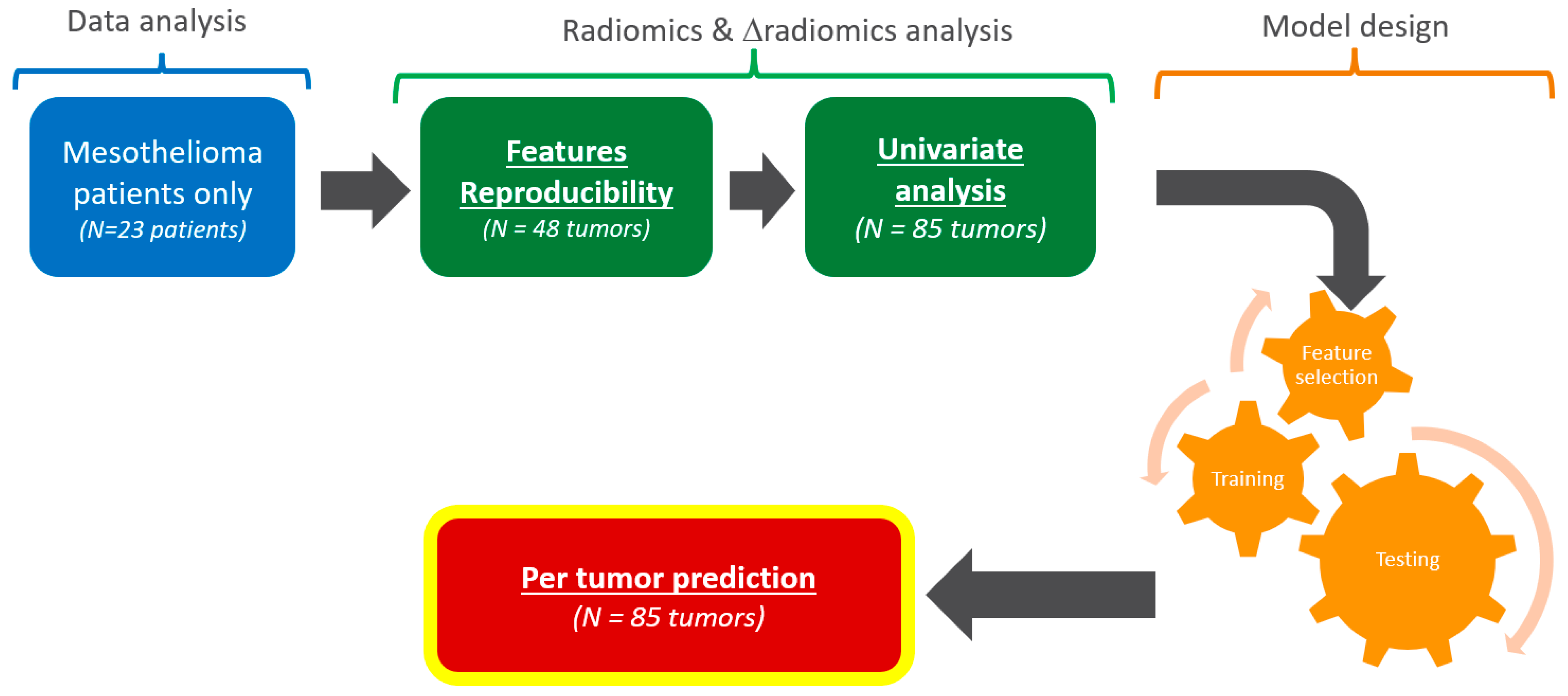
Figure 1.
Analysis workflow. From the original clinical trial, only mesothelioma patients were considered. This study consisted of a data analysis (blue), radiomics and Δradiomics analysis (green), and model design (orange). The outcome was a pilot evaluation of the predictive performances of target tumors responses.
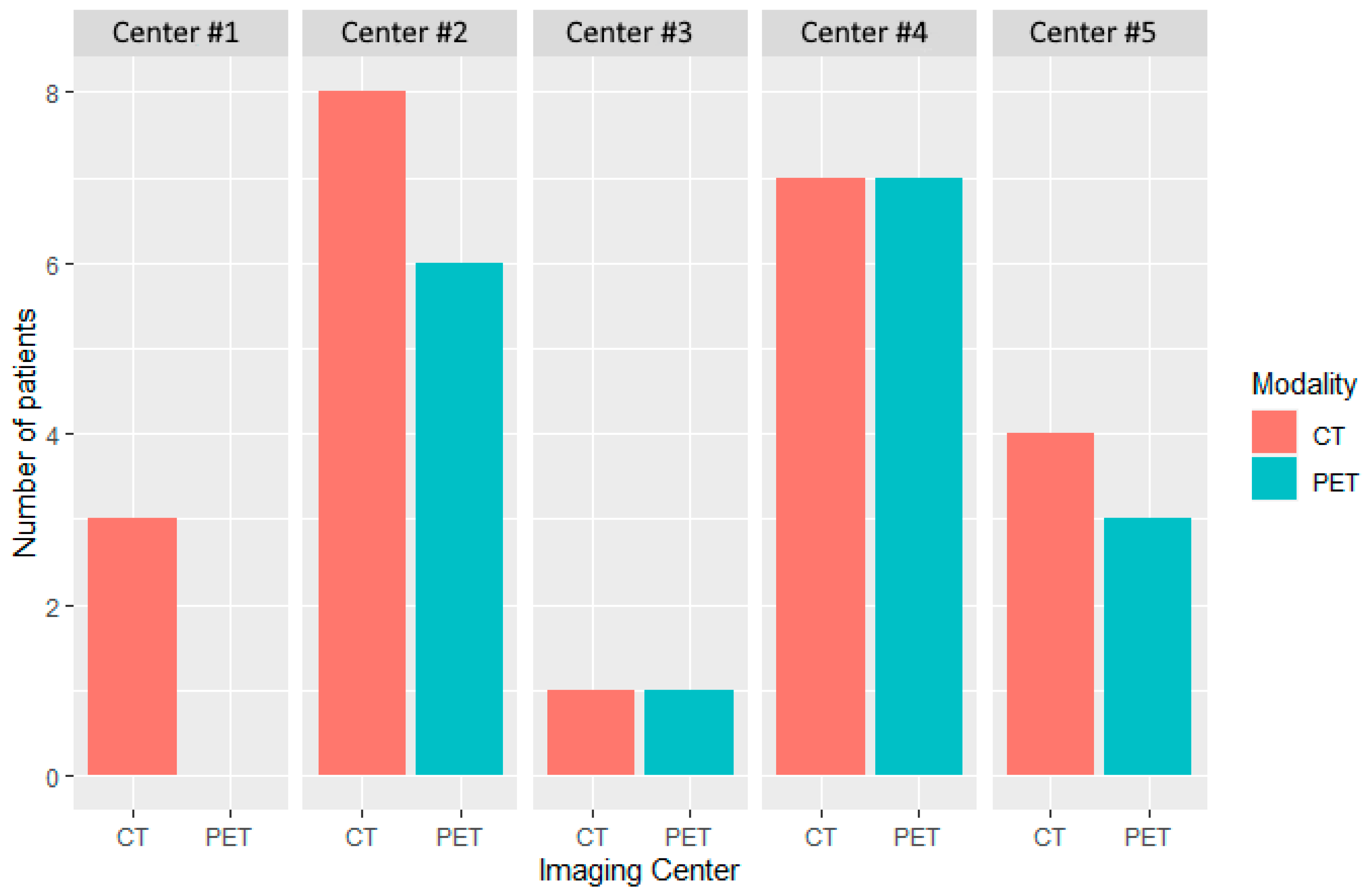
Figure 2.
Distribution of patients by modality and center at baseline. Five imaging centers participated in the evaluation of patients treated in this study. CT and PET imaging were performed in 23 and 17 patients, respectively. A single imaging center performed only CT (Center #1).
Figure 2.
Distribution of patients by modality and center at baseline. Five imaging centers participated in the evaluation of patients treated in this study. CT and PET imaging were performed in 23 and 17 patients, respectively. A single imaging center performed only CT (Center #1).
Figure 3.
Distribution of acquisition parameters at baseline. (Left) CT acquisition parameters. From inner to outer circle: manufacturer (Siemens or GE), models, Kvp (90, 120, 130), reconstruction kernel (Standard, Br40, Soft), slice thickness (2.5; 5), and voxel size (0.6; 1.0). (Right) PET acquisition parameters. From inner to outer circle: manufacturers (Siemens (Siemens Healthineers, Forchheim, Germany), GE (GE Healthcare, Milwaukee, WI, US)), models, reconstruction kernel (AllPass, XYZ Gauss (2.0, 3.5, 5.0)), slice thickness (2.0; 5.5), and voxel size (1.5; 6.9). Representativeness was deemed significant for generalization.
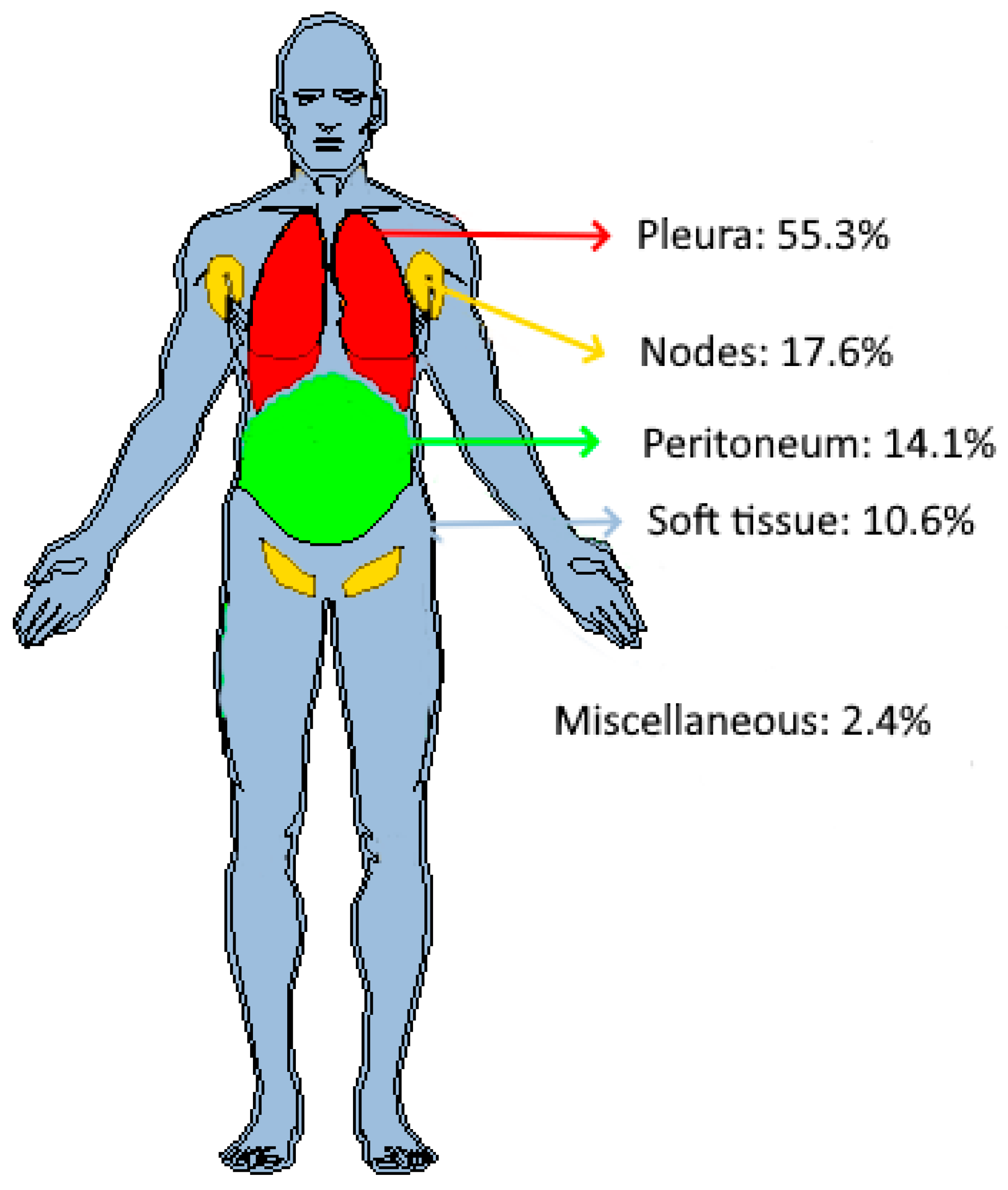
Figure 4.
Distribution of target tumors in patients’ anatomy. Out of 85 tumors, 55.3% (n = 47) were found in the pleura, 17.6% (n = 15) in the lymph nodes, 14.1% (n = 12) in the peritoneum, and 10.6% (n = 9) in soft tissues. Two additional tumors, one adrenal tumor and one liver tumor, were classified as “miscellaneous”.
Figure 5.
Radiomic/Δradiomic features according to different CCCs threshold values. The number of radiomics (a) and Δradiomics (b) were calculated for different threshold values of CCC. Radiomics reproducibility depended on tumor localization, with soft tissues (range: 238; 139) and lymph nodes (range: 43; 0) being the most and least reproducible, respectively. The reproducibility of Δradiomics depended on tumor localization, with soft tissues (range: 101; 53) and lymph nodes (range: 3; 0) being the most and least reproducible, respectively.
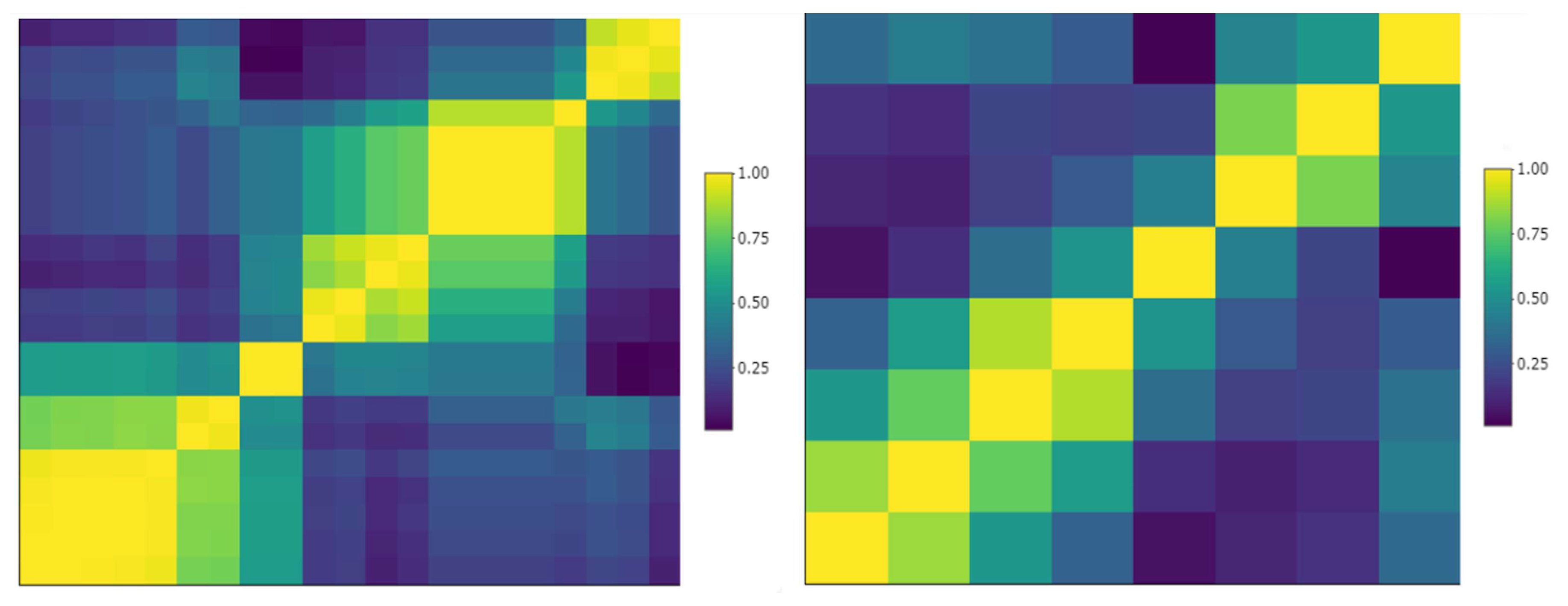
Figure 6.
Sample cluster map of reproducible pleural tumors radiomics. Left: correlation matrix of 21 radiomics that were deemed reproducible (CCC > 0.8); some of them were highly inter-correlated (yellow clusters). Right: after removing highly inter-correlated radiomics (correlation > 0.9), 8 reproducible and non-redundant pleura radiomics were preselected.
Figure 7.
Number of radiomic/Δradiomic candidates. We considered a different threshold of CCC values ranging from 0.7 to 0.9 for radiomics (a) and 0.6 to 0.9 for Δradiomics (b). For radiomics and Δradiomics, peritoneum and lymph node tumors were the most and least reproducible tumors, respectively.
Figure 7.
Number of radiomic/Δradiomic candidates. We considered a different threshold of CCC values ranging from 0.7 to 0.9 for radiomics (a) and 0.6 to 0.9 for Δradiomics (b). For radiomics and Δradiomics, peritoneum and lymph node tumors were the most and least reproducible tumors, respectively.
Figure 8.
Sample variability of segmentation and radiomics values. One pleura and one soft tissue tumor were segmented by Reader 1 and Reader 2. The volume, the joint entropy, and the sum of variance (computed from GLCM) were derived from the segmentations. The inter-reader variability of the segmentations leads to a variability in volume of 20% and 30%, in joint entropy of 16% and 7%, and in sum of variance of 41% and 56%, respectively, the pleura and the soft tissue tumors.
Table 1.
Distribution of target tumor localization by patient at baseline.
Table 1.
Distribution of target tumor localization by patient at baseline.
| Tumor Localization | Disease in Patients | Numb. of Patient with a Unique Disease |
|---|
| Pleura | 13 | 5 |
| Lymph nodes | 6 | 0 |
| Peritoneum | 8 | 3 |
| Soft tissues | 4 | 1 |
| Miscellaneous | 2 | 0 |
Table 2.
Response rate derived from tumor diameter. Response rate is presented by percentages and proportions. With a response rate of 100%, six subcategories (red) were unusable for analysis and model training.
Table 2.
Response rate derived from tumor diameter. Response rate is presented by percentages and proportions. With a response rate of 100%, six subcategories (red) were unusable for analysis and model training.
| . | Week 4 | Week 8 | Week 12 |
|---|
| Pleura | 83% (39/47) | 95% (36/38) | 97% (28/29) |
| Lymph nodes | 80% (12/15) | 91% (10/11) | 100% (10/10) |
| Peritoneum | 100% (12/12) | 100% (8/8) | 100% (2/2) |
| Soft tissues | 100% (9/9) | 100% (7/7) | 71% (5/7) |
| All | 87% (72/83) | 95% (61/64) | 94% (45/48) |
Table 3.
Response rate derived from tumor volume. Response rate is presented as percentages and proportions. Because of its limited sample size, one subcategory was unusable for analysis and model training (red).
Table 3.
Response rate derived from tumor volume. Response rate is presented as percentages and proportions. Because of its limited sample size, one subcategory was unusable for analysis and model training (red).
| . | Week 4 | Week 8 | Week 12 |
|---|
| Pleura | 30% (14/47) | 32% (12/38) | 28% (8/29) |
| Lymph nodes | 50% (7/15) | 55% (6/11) | 33% (3/10) |
| Peritoneum | 33% (4/12) | 25% (2/8) | 50% (½) |
| Soft tissues | 33% (3/9) | 28% (2/7) | 15% (1/7) |
| All | 34% (28/83) | 34% (22/64) | 27% (13/48) |
Table 4.
Response rate of Mean SUV tumors responses. Response rate is presented as percentages and proportions. Because of their limited sample size or inadequate response rate, some subcategories were unusable for analysis and model training (red).
Table 4.
Response rate of Mean SUV tumors responses. Response rate is presented as percentages and proportions. Because of their limited sample size or inadequate response rate, some subcategories were unusable for analysis and model training (red).
| . | Week 4 | Week 8 | Week 12 |
|---|
| Pleura | 20.5% (8/39) | 58% (7/12) | 36% (9/25) |
| Lymph nodes | 64% (7/11) | 100% (1/1) | 14% (1/7) |
| Peritoneum | 40% (4/10) | 34% (2/6) | 0% (0/1) |
| Soft tissues | 0% (0/7) | 0% (0/1) | 0% (0/7) |
| All | 67% (19/67) | 50% (10/20) | 25% (10/40) |
Table 5.
Radiomics associated with diameter-based response of target tumor. Number of radiomic features that had a significant difference of means between the responder/non-responder (Kruskal–Wallis test). Some subcategories were not evaluated (NA) because of the limited response rate.
Table 5.
Radiomics associated with diameter-based response of target tumor. Number of radiomic features that had a significant difference of means between the responder/non-responder (Kruskal–Wallis test). Some subcategories were not evaluated (NA) because of the limited response rate.
| Organ | Radiomics | ΔRadiomics |
|---|
| W4 | W8 | W12 | W8 | W12 |
|---|
| Pleura | 15 (N = 47) | 7 (N = 38) | 0 (N = 29) | 81 (N = 38) | 0 (N = 29) |
| Lymph nodes | 76 (N = 15) | 0 (N = 11) | NA | 0 (N = 11) | NA |
| Peritoneum | NA | NA | NA | NA | NA |
| Soft tissues | NA | NA | 1 (N = 7) | NA | 0 (N = 7) |
Table 6.
Radiomic features associated with volume-based response of target tumors. Number of radiomic features that had a significant difference of means between the responder/non-responder (Kruskal–Wallis test). Some subcategories were not evaluated (NA) because of the limited response rate.
Table 6.
Radiomic features associated with volume-based response of target tumors. Number of radiomic features that had a significant difference of means between the responder/non-responder (Kruskal–Wallis test). Some subcategories were not evaluated (NA) because of the limited response rate.
| Organ | Radiomics | ΔRadiomics |
|---|
| W4 | W8 | W12 | W8 | W12 |
|---|
| Pleura | 185 (N = 47) | 584 (N = 38) | 290 (N = 29) | 505 (N = 38) | 221 (N = 29) |
| Lymph nodes | 99 (N = 15) | 93 (N = 11) | 53 (N = 10) | 404 (N = 11) | 164 (N = 10) |
| Peritoneum | 122 (N = 12) | 55 (N = 8) | NA | 0 (N = 8) | 0 (N = 2) |
| Soft tissues | 129 (N = 9) | 2 (N = 7) | 0, (N = 7) | 2 (N = 7) | 0 (N = 7) |
Table 7.
Radiomic features associated with PERCIST response of target tumors.
Table 7.
Radiomic features associated with PERCIST response of target tumors.
| Organ | Radiomics | ΔRadiomics |
|---|
| W4 | W12 | W4 | W12 |
|---|
| Pleura | 532 (N = 39) | 209 (N = 25) | 73 (N = 39) | 71 (N = 25) |
| Lymph nodes | 282 (N = 11) | 53 (N = 7) | 48 (N = 11) | NA |
| Peritoneum | 89 (N = 10) | NA | 278 (N = 10) | NA |
| Soft tissues | NA | NA | NA | NA |


 ,
, 


