Hydrological Response of the Wami–Ruvu Basin to Land-Use and Land-Cover Changes and Its Impacts for the Future

Abstract

The evaluation of the hydrological responses of river basins to land-use and land-cover (LULC) changes is crucial for sustaining water resources. We assessed the impact of LULC changes (1990–2018) on three hydrological components (water yield (WYLD), evapotranspiration (ET), and sediment yield (SYLD)) of the Wami–Ruvu Basin (WRB) in Tanzania, using the Soil and Water Assessment Tool (SWAT). The 1990 LULC imagery was used for SWAT simulation, and imagery from 2000, 2010, and 2018 was used for comparison with modelled hydrological parameters. The model was calibrated (1993–2008) and validated (2009–2018) in the SWAT-CUP after allowing three years (1990–1992) for the warm-up period. The results showed a decrease in WYLD (3.11 mm) and an increase in ET (29.71 mm) and SYLD (from 0.12 t/h to 1.5 t/h). The impact of LULC changes on WYLD, ET, and SYLD showed that the increase in agriculture and built-up areas and bushland, and the contraction of forest led to the hydrological instability of the WRB. These results were further assessed with climatic factors, which revealed a decrease in precipitation and an increase in temperature by 1 °C. This situation seems to look more adverse in the future, based on the LULC of the year 2036 as predicted by the CA–Markov model. Our study calls for urgent intervention by re-planning LULC and re-assessing hydrological changes timely.

1. Introduction

In recent decades, changes in the hydrological processes of a wide range of river basins have been observed with increasing frequency due to global trends in human population, climate change, and underlying surface features at global, regional, and local scales [1,2,3,4]. In addition to population, climate, and underlying surface features, land-use and land-cover changes (LULCC) have a potentially large impact on hydrological processes [5,6]. These include changes in water and sediment yields [7], surface runoff, baseflow, streamflow [8,9,10,11], soil water content [12], groundwater recharge [13], and annual river discharge [14]. In most cases, the influence of LULCCs is highly visible due to the modification of dense vegetation into agriculture that, by 2017, occupied 37% of the global land surface and employed about 50% of the world population [15,16]. Despite this, in developing countries (e.g., Tanzania) where arable lands are found in river basins, such statistics are lower due to lack of land-use planning; agriculture is critical for the livelihood of more than 70% of the general population in such countries [17,18]. Vegetation can have a significant effect on hydrological fluxes due to variations in the physical characteristics of the soil and land surface, such as the roughness, albedo, infiltration capacity, root depth, architectural resistance, leaf area index (LAI), and stomatal conductance [19,20].

With respect to the hydrological responses due to LULCCs, Bessah et al. [21] found a strong relationship between land-use and land-cover (LULC) changes and extreme spatial variations in water yield in the Pra River Basin, Ghana. Mbungu and Kashaigili [22] found a decreasing trend in streamflow with the LULC changes associated with deforestation and inappropriate farming in the Little Ruaha Watershed. Santos et al. [23] reported an increase in surface runoff due to the reduction in forest areas in the large basins in the Eastern Amazon. Li et al. [24] and Guzha et al. [25] found a decrease in surface runoff in China and East African catchments, respectively, due to the increase in forests and other vegetation covers. These contradictory findings signify that LULC changes impact the hydrology of river basins differently. According to Pinto et al. [26], such differences are likely due to the ability of forest cover to retain organic matter, thereby increasing the water-holding capacity and infiltration rates of the soil. This implies that evaluating and quantifying LULCC impacts on river basin hydrology is case-specific and thus, would benefit from the use of specific modelling techniques.

To date, several models, including the Precipitation-Runoff Modelling System (PRMS), the Soil and Water Assessment Tool (SWAT), the Hydrological Engineering Centre’s Hydrologic Modelling System (HEC-HMS), the Hydrological Simulation Program-Fortran (HSPF) model, the European Hydrological System Model (MIKE-SHE), the Hydrological Catchment Model (WaSiM-ETH), and the Web-based Hydrograph Analysis Tool (WHAT) have been used to assess the impacts of LULC changes on small- and large-scale river basins [14,27,28,29,30,31,32,33,34]. Despite all these models providing outstanding results relative to the subject and data inputs, SWAT has been widely applied because of its robustness in integrating topography, soil information, LULC, and climatic variables for water resource management over wide-reaching river basins [4,35].

For example, Nie et al. [36] used the SWAT model to quantify the impacts of LULCCs on the river basin hydrology of the Upper San Pedro watershed in Mexico from 1973 to 1997. Their results indicated that the replacement of desert scrub/grassland by a mesquite invasion was the major contributor to the Upper San Pedro watershed baseflow reduction. Zhu and Li [37] examined the hydrological impacts of LULCCs in the Little River catchment in the United States using LULC data from 1984 to 2010. This study revealed that an increase in the streamflow of the Little River catchment was closely related to the LULCC of urban expansion, whereas a reduction in sediment loads was mostly related to a decrease in agricultural activities. Gashaw et al. [38] modelled the hydrological impacts of LULCCs in the Andassa watershed, part of the headstream areas of the Blue Nile River, Ethiopia, from 1985 to 2015. Their study found that the increase in cultivated land and the withdrawn forest, shrubland, and grassland areas had different impacts on the groundwater flow, surface runoff, and water yield of the Andassa watershed for different seasons. Wang et al. [39], on the other hand, evaluated the individual and combined impacts of climate and LULCCs on hydrological events in the Xitiaoxi River Basin (XRB), found in the delta of China’s Yangtze River, and projected future land-use conditions using the CA–Markov model. Their findings also indicated that the XRB is expected to experience extreme hydrological events due to the land-use and climatic conditions of the river basin. Another study by Zhang et al. [40] in Australia simulated hydrological responses to land-use change using an improved SWAT model in the North Johnstone River catchment and found that land-use change impacted hydrological variables, with the most notable impact being on surface runoff. Generally, despite their noteworthy results, these and many other studies are limited to river sub-catchments/sub-basins (i.e., the small land units of the far river systems). Thus, they lack the ability to provide insights into cumulative LULCC impacts on the hydrology of rivers.

A similar problem is also noted in Tanzania, which has a significant watershed called the Wami–Ruvu Basin (WRB) with multiple land uses. Notwithstanding the increase in multiple LULCCs and their impacts, few hydrological studies have been conducted on this basin. A study by Nobert and Jeremiah [41] focused on the Wami sub-basin to investigate the hydrological response of LULC change on water yield, surface runoff, and base flow. Wambura [42] studied the same subject in the same location, but with the one hydrological parameter of streamflow. At the other end, Natkhin et al. [43] examined discharge regimes due to LULCCs for the Ngerengere catchment of the Ruvu sub-basin.

Considering the current conditions of the WRB, namely an increasing population, a poor understanding of hydrological parameters, and insufficient coverage of the entire basin, this study was designed to investigate and assesses the LULCCs of the WRB between 1990 and 2018 in order to determine the hydrological impacts on water yield (WYLD), evapotranspiration (ET), and sediment yield (SYLD) using the SWAT model. The selection of the study years considered the availability and quality of data. We further considered using Microsoft Excel and Origin Lab for sorting and processing the different hydrological inputs for the SWAT model. An ANN for LULC classification was also used due to its great ability to produce more accurate results than others, such as the Maximum Likelihood and Mahalanobis classifiers [44]. Furthermore, we assessed the future impacts of LULCCs using the CA–Markov model. The study results are expected to provide useful information for hydrologists, land-use planners, policymakers, resource managers, and decision-makers in the WRB and in other river basins that are susceptible to LULCCs.

2. Materials and Methods

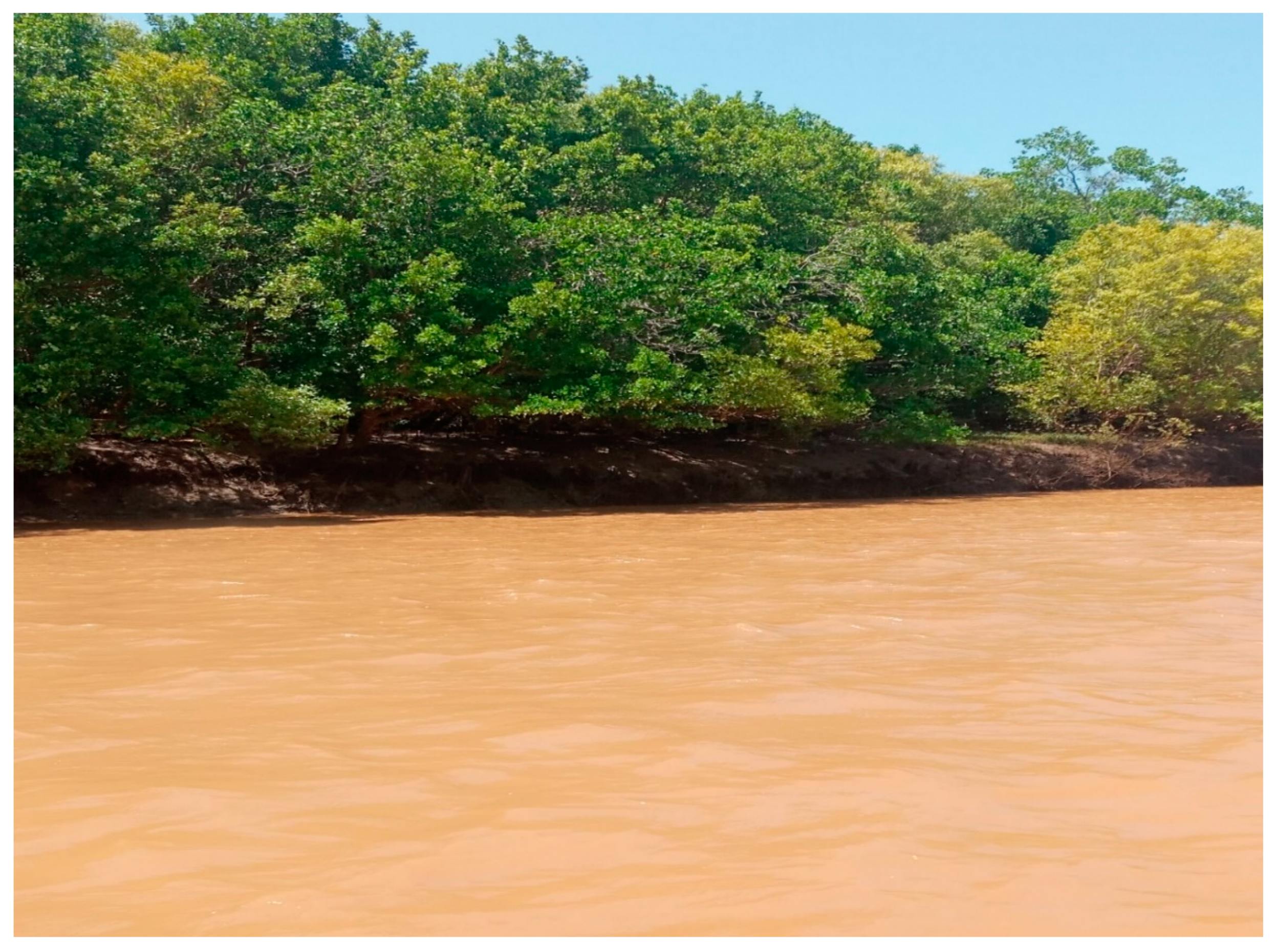
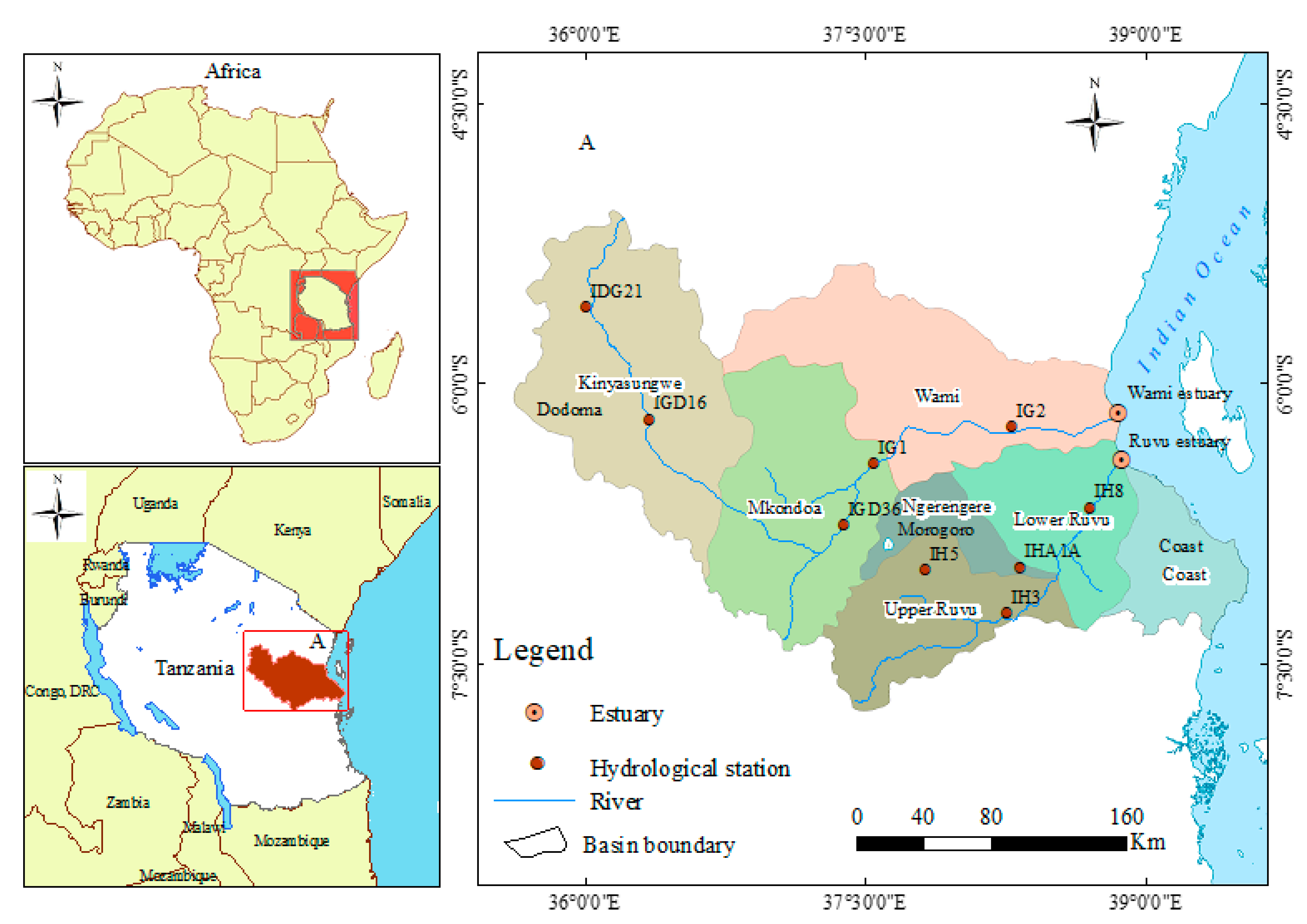
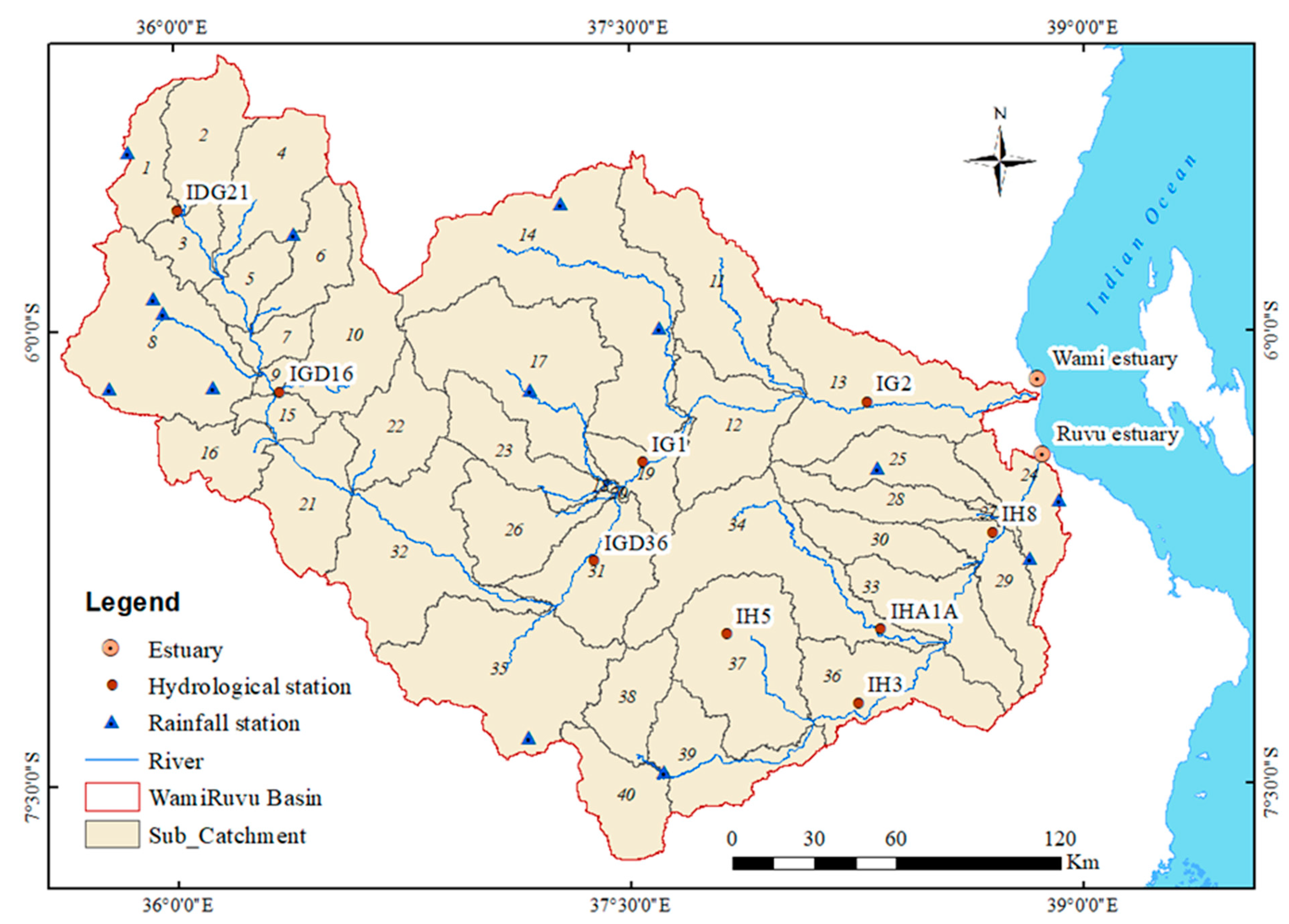
2.1. Study Area

The WRB is located between 5°–7° S and 36°–39° E in Tanzania, East Africa, (Figure 1) and encompasses a total area of approximately 66,820 km², with an altitudinal gradient of approximately 2267 m above sea level. The WRB consists of two sub-basins, the Wami sub-basin (43,946 km²) and the Ruvu sub-basin (22,874 km²), with two estuaries and seven sub-catchments of the Kinyasungwe, Mkondoa, Wami managed by the Wami sub-basin and the Upper Ruvu, Ngerengere, Lower Ruvu, and the coast managed by the Ruvu sub-basin. This basin originates in the Eastern Arc Mountain range in central Tanzania and flows eastwards across fertile agricultural plains and grassland savannah to the Indian Ocean coastline. Most of the basin area is composed of low-lying areas and a slightly elevated hilly area with moderate undulation, except for the most important hotspots of the basin: the Uluguru Mountains in the upper area of the Ruvu sub-basin (Appendix A, Figure A1 and Figure A2) and the Nguru Mountains in the upper area of the Wami sub-basin (Appendix A, Figure A3) [45,46].

The basin climate is characterised by semi-arid conditions in the western areas and a humid climate with high rainfall along the eastern areas towards the Indian Ocean. The average rainfall is approximately 500–760 mm per year in the west of the semi-arid highlands, 900–1000 mm in the central and coastal regions of the Wami sub-basin, and 800–2000 mm in the Ruvu sub-basin. The climate of the Ruvu sub-basin varies according to the topography. Most of its areas receive rainfall ranging between 800 and 1200 mm, except for the eastern slopes of the Uluguru Mountains, which have a mean annual rainfall in excess of 2000 mm, and the Ukaguru Mountains, which receive between 1000–1800 mm annually, as revealed by Kashaigili [47]. The WRB annual mean temperature ranges from 12 °C to 32 °C [48]. The basin population was estimated to be 10 million in 2018 [49]. Furthermore, according to the project conducted by the Japan International Cooperation Agency (JICA) [50], the total population in the WRB is forecasted to increase to 12.58 million in 2035.

2.2. SWAT Model Description

The SWAT hydrological model is a continuous time- and spatially-distributed basin-scale model in which hydrological processes on the surface and subsurface are coupled in order to simulate the impacts of changes in management practices [35]. It was introduced in the 1990s to assist water resource managers in assessing hydrological responses for proper management [51,52]. As a built-in program, SWAT stands for the Soil and Water Assessment Tool in computing environments. It takes different forms of naming/extension depending on the key GIS software installed with it, such as ArcSWAT for the ArcGIS software, MSWAT for Map window software, and QSWAT for QGIS software. Despite the difference in its extension, this model used the same basic algorithms guided by the water balance equation (i.e., Equation (1)). Further details can be found in [53].

$$S{W}_t=S{W}_o+{\displaystyle \sum }_{i=1}^t\left(R_i-Q_{surf,i}-E{T}_i-P_i-Q_{gw,i}\right)$$

(1)

Notes: SW_t is the final soil water content (mm), SW_o is the initial soil water content on day i (mm), t is the time in days, R_i is the amount of precipitation on day i (mm), Q_surf,i is the amount of surface runoff on day i (mm), ET_i is the amount of evapotranspiration on day i (mm), P_i is the amount of water entering the vandose zone from the soil profile on day i (mm), and Q_gw,i is the amount of return flow on day i (mm). In this study, we used ArcSWAT extension in the ArcGIS software.

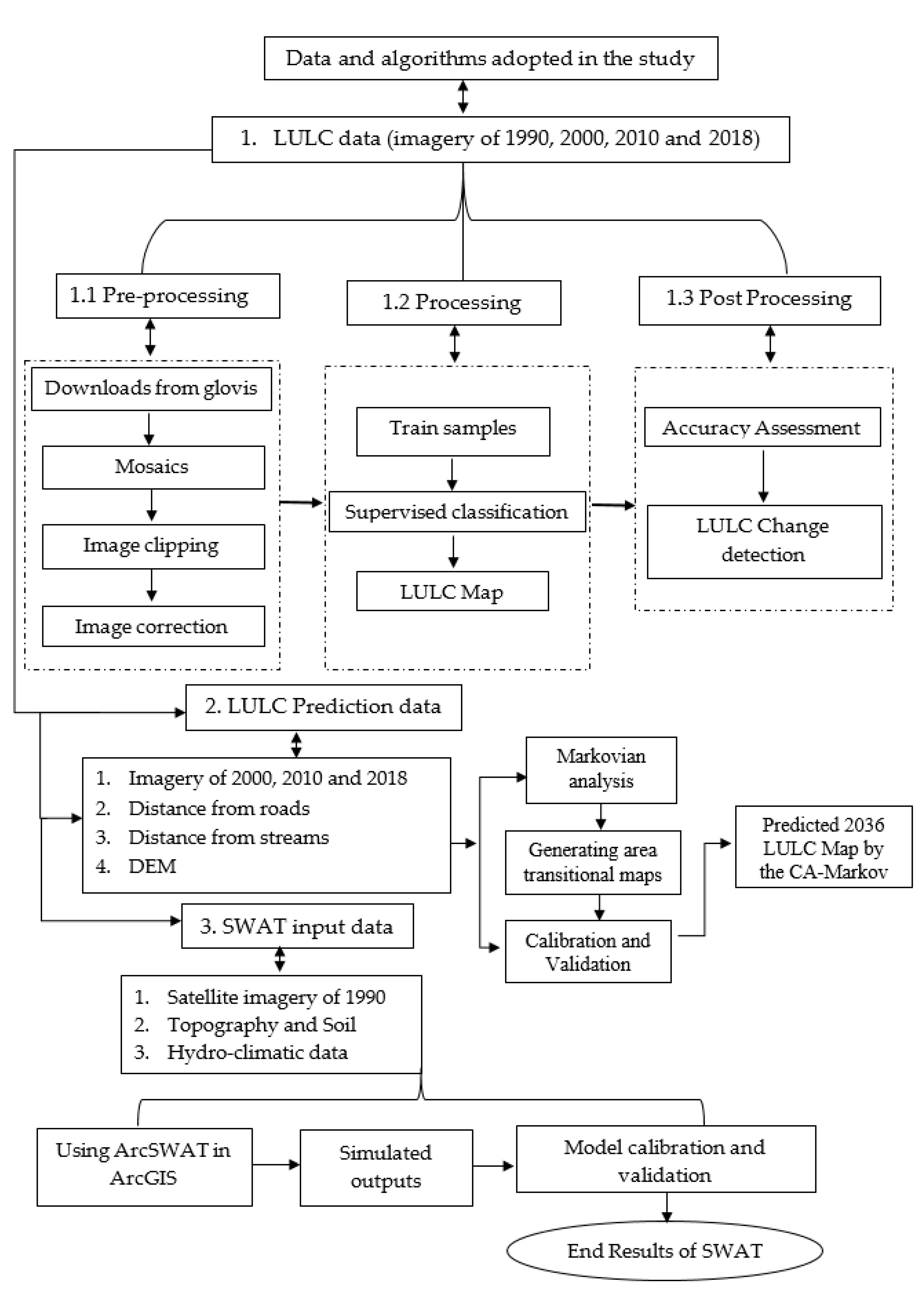
2.3. Data Requirements for the Model Input

Four types of data were required to build up the SWAT model: topography; soils; LULC data; and basic climatic data. These data were acquired from different sources and were fit for the appropriate model inputs; each was pre-processed as explained below.

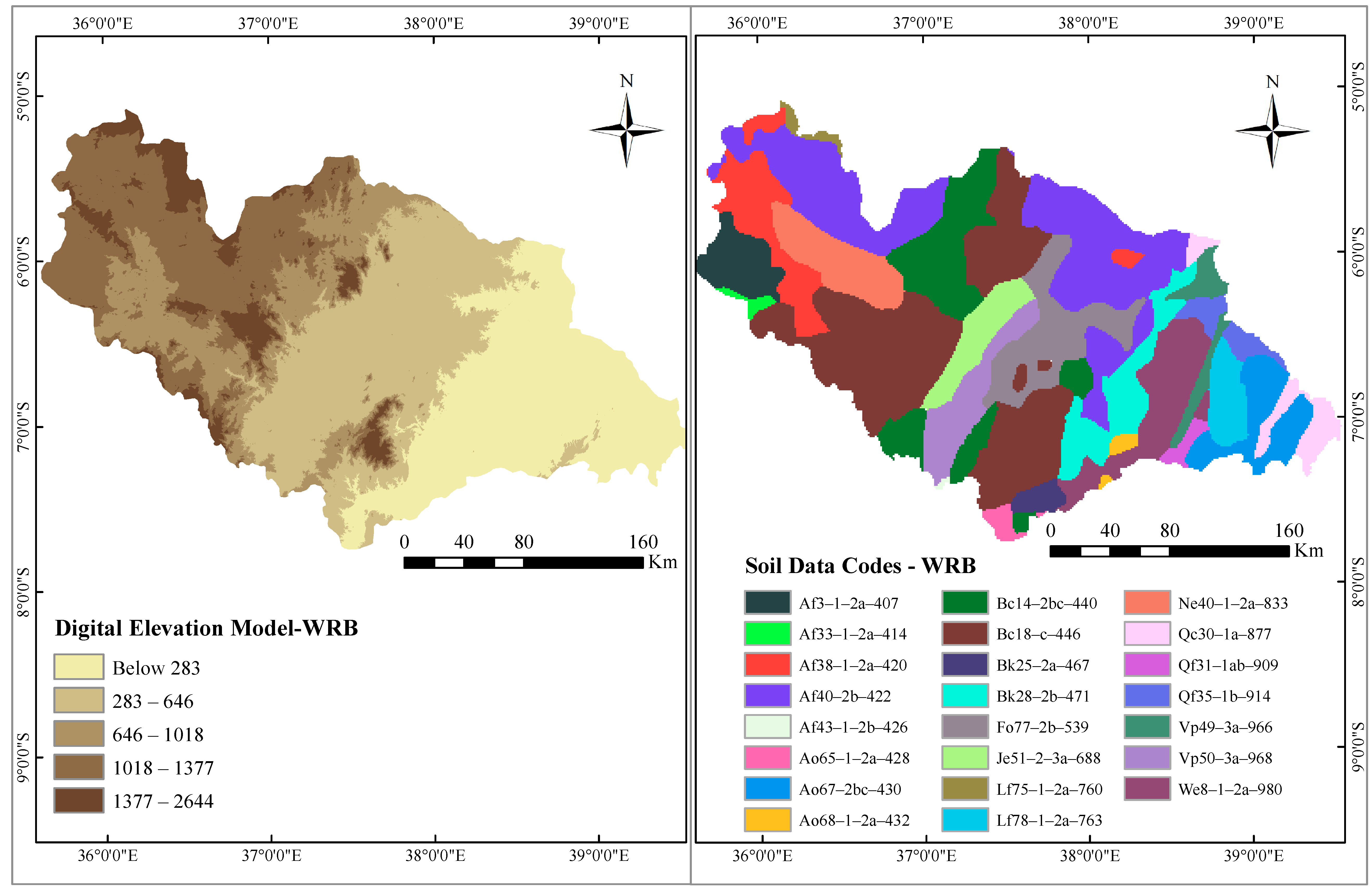
2.3.1. Topography and Soil Data

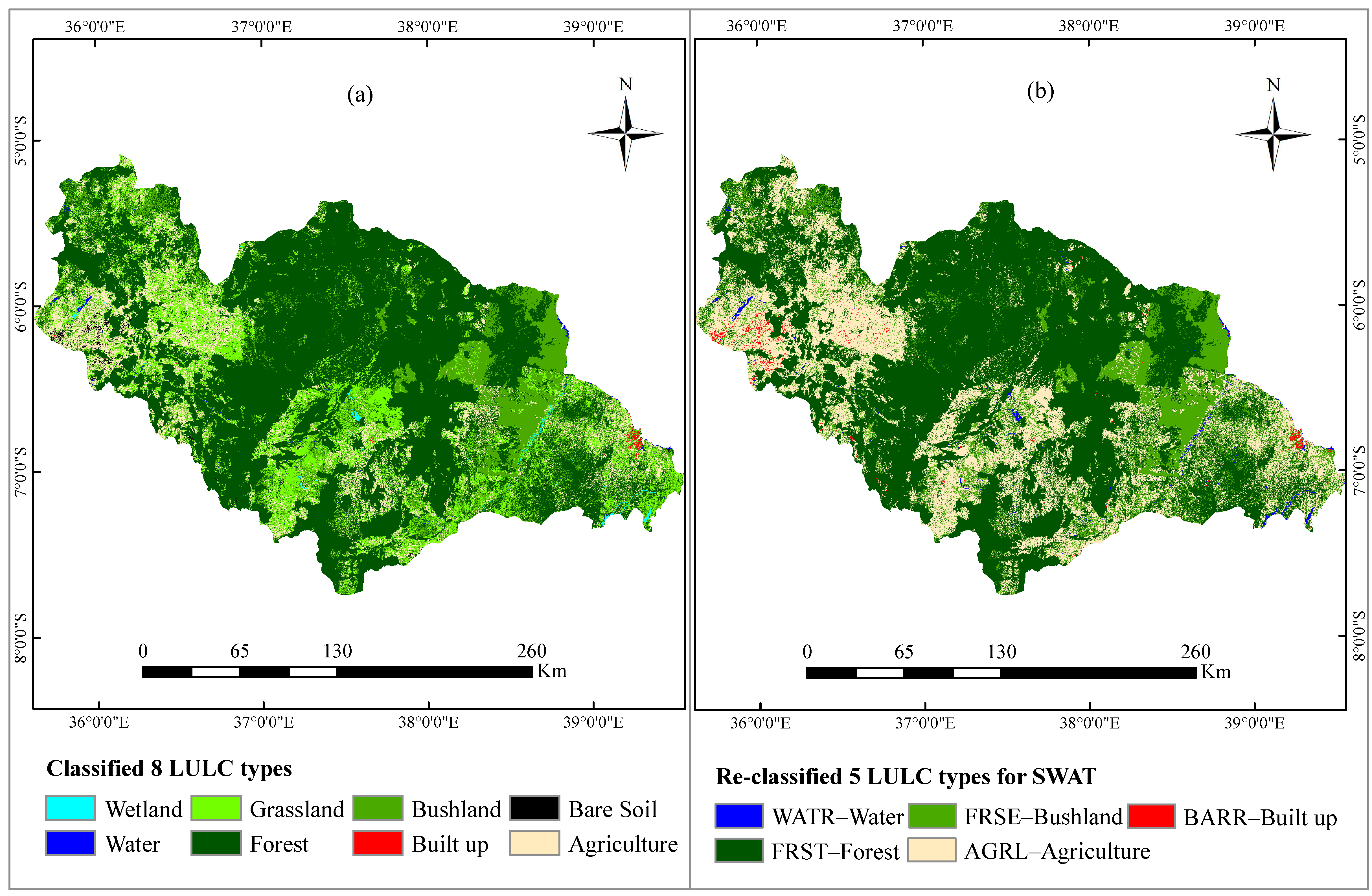
The topographical data were extracted from the digital elevation model, mapped by the Advanced Land Observing Satellite (ALOS) using the Panchromatic Remote-sensing Instrument for Stereo Mapping (PRISM) with a horizontal resolution of 30 m [54]. The choice of the ALOS DEM was made because of its highly accuracy results that have been tested in many countries such as Russia [55], Argentina [56], the Philippines [57], and Cameroon [58], which is close to the case study area. The topographic data were used to generate the stream networks of the WRB, including river length, slope, and width.

The soil data were retrieved from the Agricultural Organization (FAO) and used to determine soil parameters, such as texture, hydrologic soil group, and the available water content of the soil, as needed to run the SWAT model [59]. These data were available in the GIS shapefile form covering all over the world, and its soil codes matched the MSWAT extension. Thus, we added a new column to the ArcSWAT database for the soil data with names similar to those from the downloaded shapefile and used it when defining the hydrological response units (HRUs). In general, the soil data used in this study were chosen due to their high accuracy and wide use in many studies, such as in the Karnali River Basin of Nepal’s Himalaya [60], Giba catchment, Tigray, Ethiopia [61], and in the Wami sub-basin—A part of the WRB in Tanzania by [62]. Figure 2 shows the topographical and soil data used for the model input.

Table 1. The major soil types existing in the WRB and their descriptions.

SN/Value	Soil Codes	Soil Definition
1	Af3-1-2a-407	Sandy clay loam
2	Af33-1-2a-414	Sandy loam
3	Af38-1-2a-420	Sandy loam
4	Af40-2b-422	Sandy clay loam
5	Af43-1-2b-426	Sandy loam
6	Ao65-1-2a-428	Sandy loam
7	Ao67-2bc-430	Sandy clay loam
8	Ao68-1-2a-432	Sandy loam
9	Bc14-2bc-440	Loam
10	Bc18-c-446	Loam
11	Bk25-2a-467	Loam
12	Bk28-2b-471	Loam
13	Fo77-2b-539	Sandy clay loam
14	Je51-2-3a-688	Clay loam
15	Lf75-1-2a-760	Sandy clay loam
16	Lf78-1-2a-763	Sandy loam
17	Ne40-1-2a-833	Sandy clay loam
18	Qc30-1a-877	Sandy loam
19	Qf31-1ab-909	Sandy loam
20	Qf35-1b-914	Sandy loam
21	Vp49-3a-966	Clay
22	Vp50-3a-968	Clay
23	We8-1-2a-980	Sandy clay loam

provides a detailed description of the soil data types in the WRB.

2.3.2. LULC Data

The data for LULCs were obtained from Landsat satellite imagery, shared by the United States Geological Survey [63]. The data were downloaded at https://glovis.usgs.gov (accessed on 18 July 2021) from six Landsat scenes along WRS-2 paths 166 to 168 and rows 64 and 65 for 1990, 2000, 2010, and 2018. These datasets were retrieved from three different sensors of TM, ETM, and OLI during the dry season and with the threshold of less than 10% for cloud cover. The choice of this source of imagery was based on their availability that covers the full length of the studied time, the same spatial resolution of 30 m, and common Red–Green–Blue bands, enhancing the visual interpretation during classification. The 1990 imagery was used as a direct input for the simulation of the SWAT model for 29 years and hence, to provide a better understanding, we used the rest of the imagery for the comparative analysis of the modelled hydrological parameters, as detailed in the subsequent sections. The details of the dates, Landsat, and sensors of the downloaded data are presented in

Table 2. The Landsat satellite imageries used in the WRB.

Date	Satellite	Sensor	Path/Row	Date	Satellite	Sensor	Path/Row
30 July 1990	Landsat 5	TM	168/64	1 July 2010	Landsat 5	TM	166/64
1 August 1990	Landsat 5	TM	167/64	6 July 2010	Landsat 5	TM	167/65
4 August 1990	Landsat 5	TM	166/64	27 June 2010	Landsat 5	TM	166/65
5 August 1990	Landsat 5	TM	168/65	29 June 2010	Landsat 5	TM	167/64
7 August 1990	Landsat 5	TM	167/65	15 July 2010	Landsat 5	TM	168/64
8 August 1990	Landsat 5	TM	166/65	20 July 2010	Landsat 5	TM	168/65
26 July 2000	Landsat 7	ETM+	168/65	16 August 2018	Landsat 8	OLI	168/64
19 July 2000	Landsat 7	ETM+	168/64	17 August 2018	Landsat 8	OLI	167/64
15 June 2000	Landsat 7	ETM+	167/64	19 August 2018	Landsat 8	OLI	166/64
21 June 2000	Landsat 7	ETM+	166/64	20 August 2018	Landsat 8	OLI	168/65
30 June 2000	Landsat 7	ETM+	166/65	1 September 2018	Landsat 8	OLI	167/65
7 July 2000	Landsat 7	ETM+	167/65	2 September 2018	Landsat 8	OLI	166/65

. All Landsat scenes were atmospherically corrected using FLAASH in ENVI 5.3 software through radiometric calibration and dark subtraction processes, and their digital numbers were converted into the top of atmosphere reflectance before being mosaicked into a single composite image cropped to the study area for LULC classification. To determine the LULC types, we identified training datasets and used a classifier selection tool to encode the sampling data for the classification process. The training datasets were randomly divided into two subsets: 60% was used for the training of the classifier and 40% was used for the accuracy assessment. Finally, the images were classified using artificial neural networks (ANNs). An ANN is a supervised classification method composed of several small processing units imitated with artificial neurons, and it is widely applied in recognition processes, such as LULC classification [64]. Eight LULC types were obtained from this process, as shown in

Table 3. The land-cover types targeted for mapping.

SN	Land-Cover Type	Description	Sample Area Recognition
1	Agriculture	Crop fields and fallow lands	Light green colour
2	Bare soil	Exposed soil and barren lands	Brown colour
3	Built-up areas	Housing, industries, transportation, and mixed urban	Purple/silver colour
4	Bushland	Land mainly comprised plants and open bush	Moderate green colour
5	Forest	Tree crown cover, woodland, and thickets	Dark green colour
6	Grassland	Mainly composed of grass	Brown/Light green colour
7	Water	Rivers, open water, lakes, ponds, and water reservoirs	Blue colour
8	Wetland	Stagnant water bodies, swamps, and marshes	Light blue colour

. The classified imagery was further assessed for accuracy using Kappa coefficient analysis by comparing the pixel information to Google Earth and sentinel−2 at 10 m spatial resolution. The overall accuracy assessment was 80.8% for the LULC images in 1990, 78.9% in 2000, 88.4% in 2010, and 86% in 2018. These results are similar to those obtained in other studies, such as those by Abineh and Bogale [65] and Rwanga and Ndambuki [66]. For the use of the LULC imagery in the model, the LULC types were required to match the SWAT code database. Thus, we encoded them accordingly, as shown in Figure 3.

Furthermore, to understand the patterns of LULC under future hydrological impacts, we used the CA–Markov model in the Land Change Modeller in the Terrset 18.31. The choice of the CA–Markov model was considered based on its wide application in the modelling, simulation, and prediction of the different dimensions of LULC change [67,68,69]. Overall, the process of predicting LULC involved three steps: (1) carrying out a CA–Markovian chain analysis of the 2000 and 2010 LULC maps to generate transition area matrices; (2) generating transitional area maps of LULC; (3) validating and calibrating the accuracy of the model by simulating the 2018 LULC map based on Kappa indices. Finally, with the calibrated and validated CA–Markov model, the 2018 LULC map (reference map) was used to simulate the future patterns of the year 2036. This prediction was simulated based on the number of interactions between 2000 and 2018 (18 years).

2.3.3. Hydroclimatic Data

The observed climatic data used in this study include the daily precipitation, temperature, wind speed, relative humidity, and solar radiation, which were obtained from the Tanzania Meteorological Agency (TMA), the University of Dar es Salaam-Water Resources Engineering Department database, and the Ministry of Water, Dodoma. All these data were sorted and processed in Excel for use in the SWAT model and, in order to obtain prior knowledge of the basin hydrology, the basic data of precipitation and temperature were assessed to determine their trends using OriginLab. For calibration and validation purposes, the flow data at the outlets of the sub-basin (1H8 and IG2) with 37% of missing data [70] were used in this study. These data cover a period of 29 years (1990–2018) and were collected from the WRB office in the Morogoro region. The choice of the use of the IG2 and 1H8 outlets was due to the quality of their data as indicated in many previous studies, such as [41,70], and to topography, as they are both found downstream. Thus, they are the main collectors of the entire streamflow of the basin. Detailed information on the outlets is presented in

Table 4. The station-outlets used for the SWAT model calibration and validation.

Station-Outlet Number	Station-Outlet Name	Data Variable	Latitude	Longitude	Elevation (m)
IG2	Wami River, Mandera	Flow	−6.2464	38.3874	75.0
1H8	Ruvu River, Morogoro Road Bridge	Flow	−6.6929	38.7081	229

. Figure 4 is a flowchart used for processing all data used in this study.

2.4. Model Set-Up and Evaluation Approach

2.4.1. SWAT Model Input

The SWAT modelling process began with watershed delineation based on digital elevation models (DEMs) using ArcSWAT in ArcGIS software. The watershed delineation involved five stages: DEM setup; stream definition; outlet and inlet definition; watershed outlet (s) selection; and the definition and calculation of the sub-basin parameters. Based on the topographical nature of the basin, both delineated stream and sub-stream networks were composed within the Wami and Ruvu sub-basins. Their outlets were also the same, coded as FLOW_OUT_13 and FLOW_OUT_24 for IG2 and 1H8, respectively (Figure 5). Subsequently, the slope information obtained from the delineation process and the other soil and land-use data allowed us to define and compute the HRUs of the WRB. This step yielded 40 HRUs, which were, in principle, the result of the overlays of the identified data characteristics [71]. It is worth noting that in each HRU, water balance was the driving force behind all processes, such as surface and groundwater flow, the interception of precipitation, and the distribution of water in different soil profiles, and could impact the movement of sediments. Moreover, as defined by the HRUs, the SWAT model required critical threshold values for land-use, soil type, and slope, and the default values for most applications were 20% for land-use, 10% for soil, and 20% for slope [72]. The default values were applied sequentially during the definition of the HRUs to limit the number of HRUs in the WRB. Finally, before we ran the model, the SWAT model required the input of the climatic data that we imported to work with the HRU information in order to obtain the final results.

2.4.2. Model Performance and Evaluation

After the simulation, the SWAT model was calibrated and validated using monthly flow data for the two gauging stations IG2 and 1H8 for FLOW_OUT_13 and FLOW_OUT_24, respectively. The flow data at the outlets of sub-basins IG2 and 1H8 were considered because this was the only hydrological data available from the WRB from 1990 to 2018. The model calibration (1993–2008) and validation (2009–2018) periods were carried out by comparing the simulated and measured flow data, with the period of (1990–1992) left out as a warm-up period. Manual and auto-calibration routines [73] were performed. Manual calibration was performed to reduce the acceptable parameter ranges at each station [4]. The optimised parameter ranges suggested by the SWAT user’s manual and other studies, such as those conducted by [74,75], were incorporated into a recently developed semi-auto-calibration approach, SUFI-2, in the SWAT-CUP [76]. The sequential uncertainty fitting II (SUFI-2) [77] method calibration and uncertainty program [73] was used, with the Nash–Sutcliffe efficiency (NSE) [78], as the objective function to identify the most sensitive parameters to be calibrated in the WRB. The details of the statistical evaluation methods that include the NSE, the ratio of the root, mean square error to the standard deviation of measured data (RSR), and the percent bias (PBIAS) are presented in

Table 5. The SWAT statistical equations used for calibration and validation processes and their level of performance.

Statistical Equation	Value	Rating Performance
$\mathrm{NSE}=1-\left[\frac{{{\displaystyle \sum }}_{1=1}^n{(Xob\left(1\right)-Ymodel\left(1\right))}^2}{{{\displaystyle \sum }}_{1=1}^n{(Xobs\left(1\right)-Xobs)}^2}\right]$	>0.65	Very good
	0.54 to 0.65	Adequate
$\mathrm{RSR}=\frac{\sqrt{{{\displaystyle \sum }}_{1=1}^n{(Xobs\left(1\right)-Ymode\left(1\right))}^2}}{\sqrt{{{\displaystyle \sum }}_{1=1}^n{(Xobs\left(1\right)-Xobs)}^2}}$	>0.50	Satisfactory
	0.00 < RSR < 0.50	Very good
	0.50 < RSR < 0.60	Good
	0.60 < RSR < 0.70	Satisfactory
	RSR > 0.70	Unsatisfactory
$\mathrm{PBIAS}=\left[\frac{{{\displaystyle \sum }}_i^n=1^{\left(Xobs\left(1\right)-Ymode\left(1\right)\right)}}{{{\displaystyle \sum }}_i^n=1^{\left(Xobs\left(1\right)\right)}}\times 100\right]$	>0.50	Satisfactory
	<±20%	Good
	±20% to ±40%	Satisfactory
	>±40%	Unsatisfactory

, and further details can be obtained from Moriasi et al. [79] and Moriasi et al. [80].

3. Results

The results of this research are presented in three phases: one for the LULCCs that are real and simulated based on the CA–Markov model, and two for the identified trends of the basic climatic data and the hydrological components modelled in the SWAT model. The results of the first and second phases are presented in a straightforward manner, as described in the methodology. The SWAT model results for each hydrological component were generated annually for the entirety of the study period; thus, for a better understanding, we chose the years 1990, 2000, 2010, and 2018 to compare the detected land-use and land-cover changes.

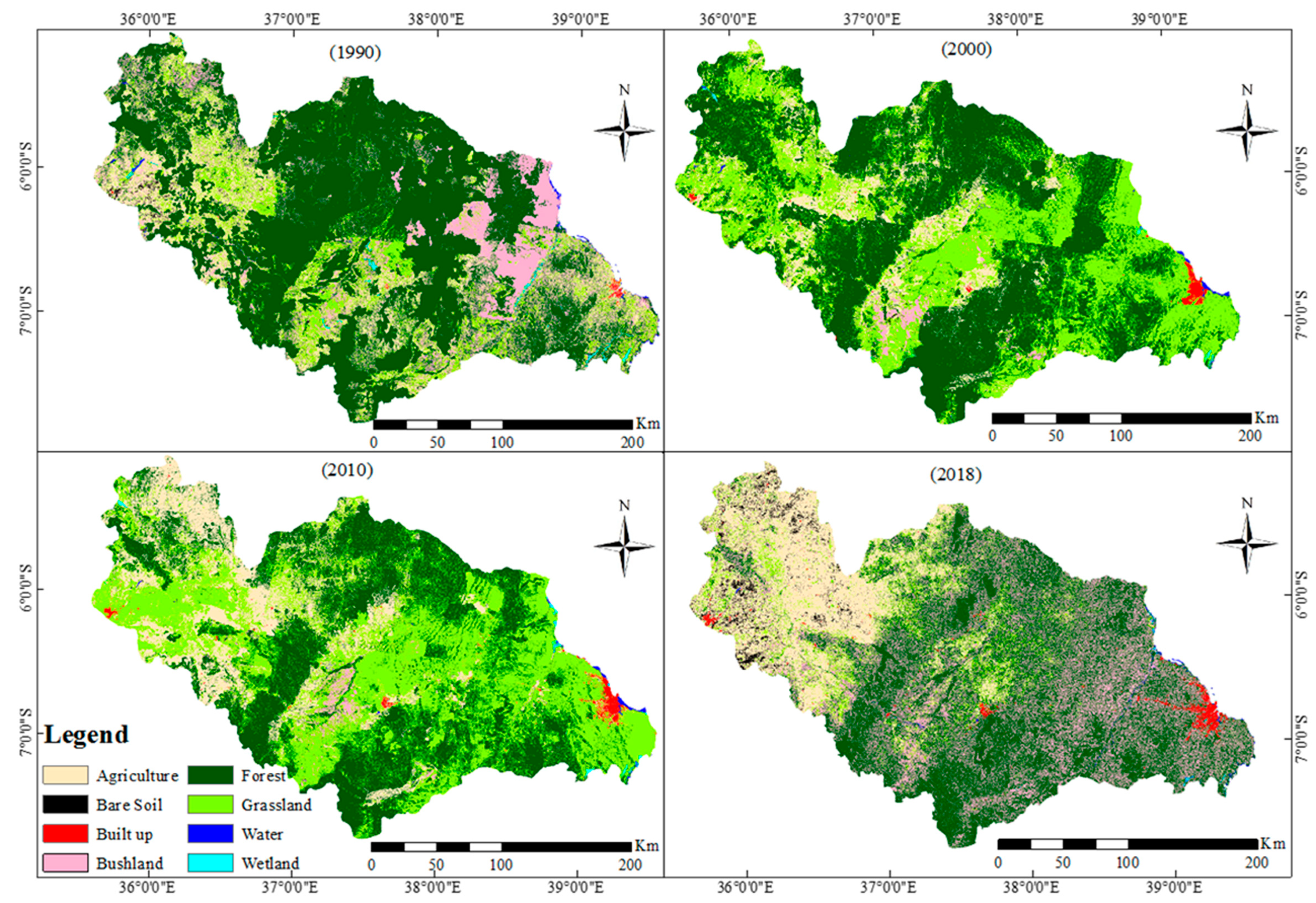
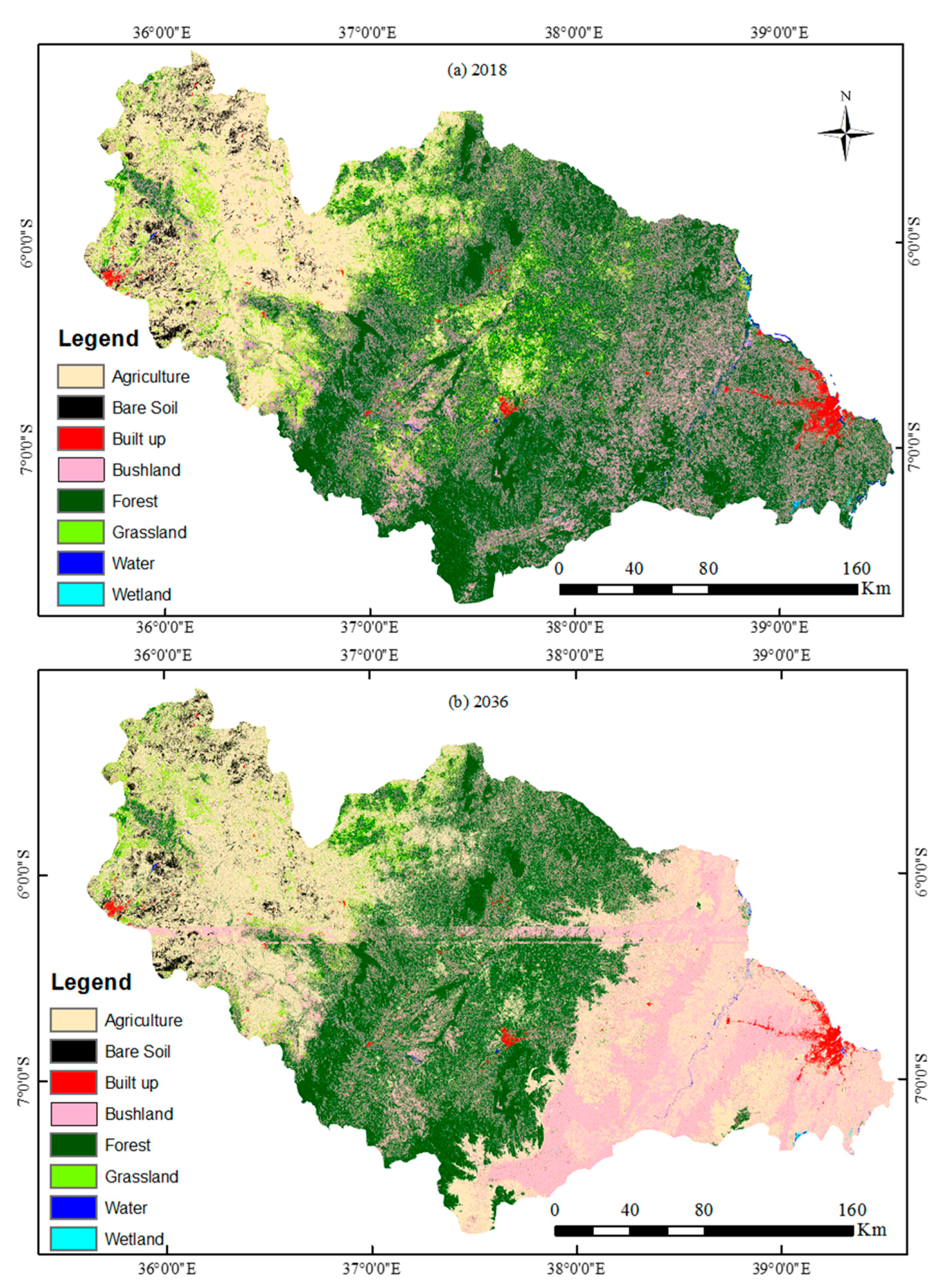
3.1. Trends of LULCCs

Table 6. The overall areas of individual LULC classification in the years 1990, 2000, 2010, and 2018 in the WRB.

LULC Types	1990 ha %		2000 ha %		2010 ha %		2018 ha %
Agriculture	705,415	10.6	772,034	11.5	990,486	14.8	1,482,554	22.2
Bare Soil	25,179	0.4	8083	0.1	25,179	0.4	135,736	2.0
Bushland	1,116,020	16.7	575,409	8.6	617,091	9.2	1,665,843	24.9
Forest	3,885,749	58.1	3,236,114	48.4	2,980,920	44.6	2,857,658	42.7
Grassland	908,883	13.6	2,029,882	30.4	2,002,217	30.0	464,219	6.9
Built-up Areas	7226	0.1	34,371	0.5	48,499	0.7	60,560	0.9
Water	19,435	0.3	17,527	0.3	13,634	0.2	13,220	0.2
Wetland	17,114	0.3	11,601	0.2	6995	0.1	5231	0.1
Total	6,685,021	100	6,685,021	100	6,685,021	100	6,685,021	100

and

Table 7. The yearly interval results of the LULC classification images for 1990–2000, 2000–2010, 2010–2018, and 1990–2018, showing area change (+Gain and -Loss) in hectares (ha) and percentage (%) in the WRB.

LULC Type	1990–2000 ha %		2000–2010 ha %		2010–2018 ha %		1990–2018 ha %
Agriculture	66,619	1.0	218,452	3.3	492,068	7.4	777,139	+11.6
Bare Soil	−17,096	−0.3	17,096	0.3	110,557	1.7	110,557	+1.7
Bushland	−540,611	−8.1	41,682	0.6	1,048,752	15.7	549,823	+8.2
Forest	−649,635	−9.7	−255,194	−3.8	−123,262	−1.8	−1,028,091	−15.4
Grassland	1,120,999	16.8	−27,665	−0.4	−1,537,998	−23.0	−444,664	−6.7
Built-up Areas	27,145	0.4	14,128	0.2	12,061	0.2	53,334	+0.8
Water	−1908	0.0	−3893	−0.1	−414	0.0	−6215	−0.1
Wetland	−5513	−0.1	−4606	−0.1	−1764	0.0	−11,883	−0.2

summarise the temporal trends of the LULCC analysis from 1990 to 2018 based on eight targeted LULC types. The spatial representation of each LULC from 1990 to 2018 is shown in Figure 6. Initially, the temporal trend of LULC in 1990, as indicated by the percentage of the total area of the WRB, was dominated by forest (58.1), followed by bushland (16.7), grassland (13.6), agriculture (10.6), water and wetland (0.6), bare soil (0.4), and built-up areas (0.1). This trend varied significantly for all LULC types in the years 2000, 2010, and 2018, as highlighted by the land covered by grassland and bushland areas (Table 6). Grassland areas increased tremendously in 2000 and declined tremendously in 2018. In contrast, bushland was the only natural area that increased from 16.7% in 1990 to 24.9% in 2018, despite a decrease in 2000 (Table 7).

Moreover, the trend of LULCC indicates a general decrease in natural areas, including forests (15.4%), grasslands (6.7%), and water and wetland cover (0.3%) (Table 7). On the other hand, the land uses supporting economic activities and population development increased, as indicated by agriculture and built-up areas (Figure 6). Taken altogether, agriculture is the LULC with the highest gain (11.6%) and forest is the LULC with the highest loss (15.4%) over the yearly intervals from 1990 to 2018 (Table 7). These LULC results agree with the results of a previous study conducted by Twisa and Buchroithner [81] in the Wami sub-basin.

On the other hand, the trends of LULC simulated by the CA–Markov model show that the main land-use classes of agriculture, built-up areas, and forest agree with real land-use changes observed previously (

Table 8. The CA–Markov model LULCC results for the year 2018, 2036 (projected), and 2018–2036, showing area change (+Gain and −Loss) in the WRB.

LULC Types	2018 ha %		2036 ha %		2018–2036 ha %
Agriculture	1,482,554	22.2	2,071,244	31.0	+588,690	8.8
Bare Soil	135,736	2.0	122,170	1.8	−13,566	−0.2
Bushland	1,665,843	24.9	1,814,294	27.1	+148,451	2.2
Forest	2,857,658	42.7	2,229,228	33.3	−628,430	−9.4
Grassland	464,219	6.9	343,206	5.1	−121,013	−1.8
Built-up Areas	60,560	0.9	92,674	1.4	+79,454	0.5
Water	13,220	0.2	8348	0.1	−4872	−0.1
Wetland	5231	0.1	3857	0.1	+148,451	2.2
Total	6,685,021	100.0	6,685,021	100.0	−1374	0.0

). These results were confirmed based on the relative accuracy (Kno = 0.8425, Klocation = 0.8357, Kstandard = 0.7987) between the classified map of 2018 and the modelled maps of 2036, as shown in in Figure 7.

3.2. Precipitation and Temperature Trends

The results of the precipitation and temperature studies from the Wami and Ruvu sub-basins showed an increase in temperature and a decrease in precipitation (Figure 8). The Wami sub-basin temperature varied between 30.5 °C and 32 °C from the 1990s to 2018. However, the Ruvu sub-basin increased from 28.5 °C to 29.5 °C. The variations in the temperature in these sub-basins demonstrate that the WRB temperature increased by approximately 1 °C from the 1990s to 2018 (Figure 8). Similarly, there was a sharp decrease in precipitation for both sub-basins during the study period. These trends were punctuated with concurrent events, such as in 1997, when both sub-basins recorded the highest precipitation, and in 2003 and 2010, when the same sub-basins recorded the lowest precipitation over the entire study period.

3.3. SWAT Simulated Outputs

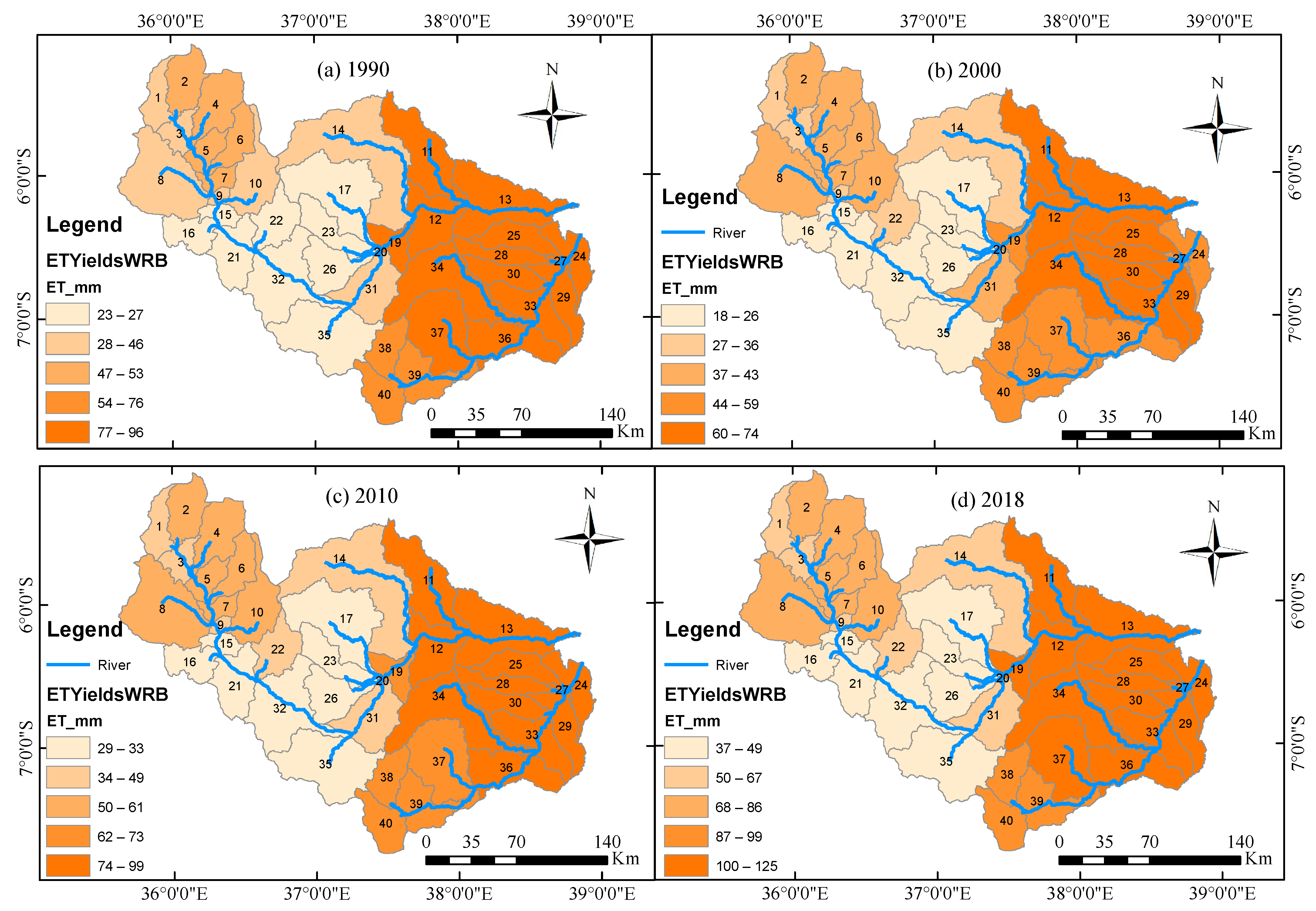
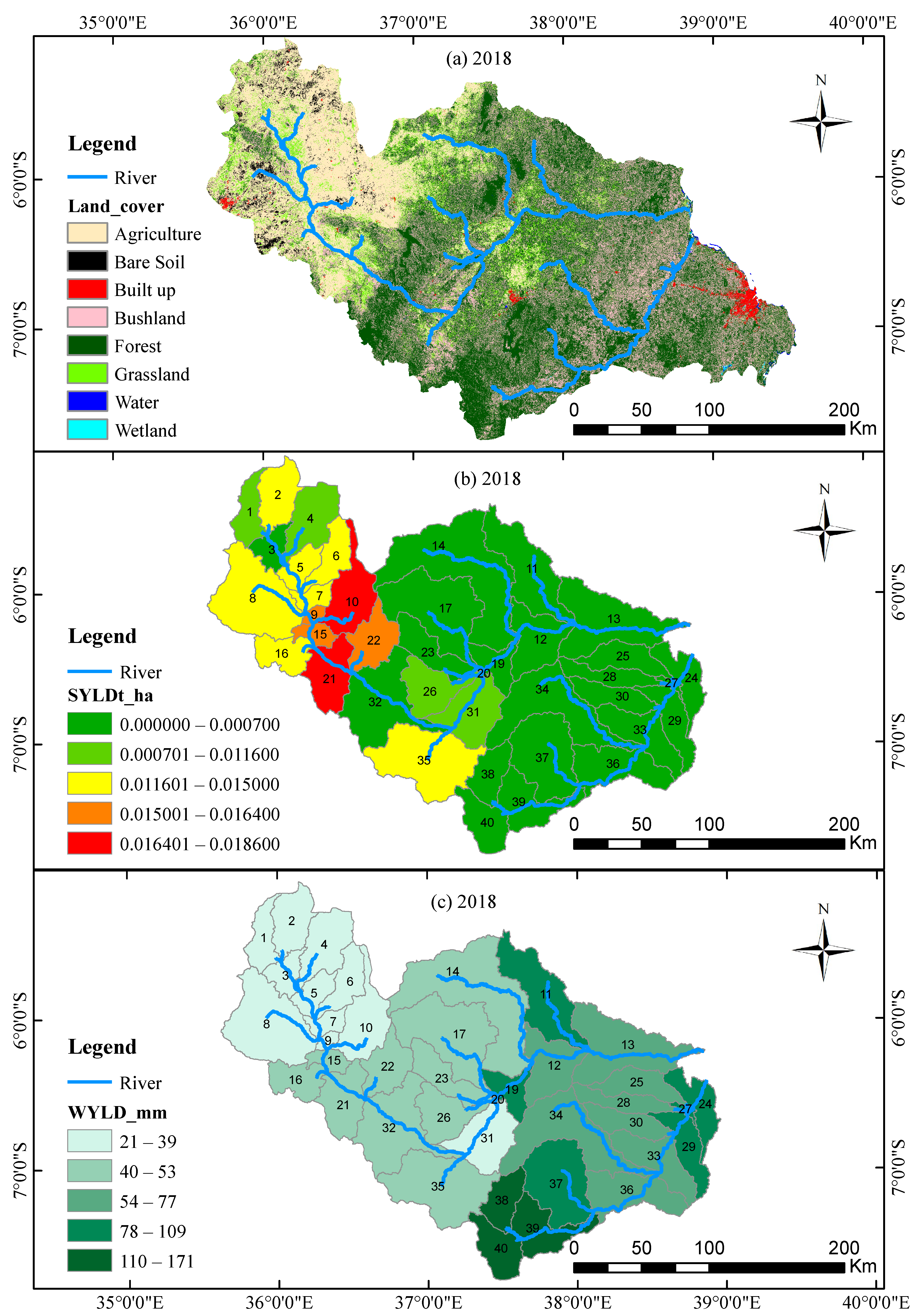
3.3.1. Spatio-Temporal Water Yield (WYLD) Distribution

Spatially, the results of the WYLD distribution show an annual variation between the four years specified by the study methods (Figure 9). These results also comprise the temporal trends for each sub-basin, which indicates a reduction in WYLD from 169.38 mm to 166.27 mm, and from 173.59 mm to 170.54 mm for the Wami and Ruvu sub-basins, respectively (

Table 9. The long-term simulation results of WYLD and its major components in the WRB.

Hydrological Component	Wami Sub-Basin		Ruvu Sub-Basin
	1990	2018	1990	2018
WYLD (mm)	169.38	166.27	173.59	170.54
Surface runoff (mm)	67.61	70.84	73.63	77.74
Groundwater flow (mm)	89.45	87.76	102.83	99.92

). The SWAT-defined WYLD was the aggregate sum of water leaving the HRU and entering the principle channel during the time step, i.e., including surface runoff and ground water flow [82]. The WYLD results also comprise the major components of surface flow and groundwater recharge, which revealed the increase in surface flow and decrease in groundwater flows for both sub-basins (Table 9). Similar results were obtained in previous studies by Nobert and Jeremiah [41] and Twisa [75], who used a section of the Wami sub-basin to study the effects of LULCCs on hydrology. In general, the results for the spatial pattern of WYLD in Figure 9 show that most of the agricultural areas in the western areas of the WRB have low water yields. These results indicate that the significant increase in LULCCs associated with expanding agricultural areas that draw water for irrigation has an impact on the changes in WYLD in the WRB (see Figure 6 and Figure 9 for comparison). Correspondingly, our study associated the WYLD reductions with the semi-arid climatic conditions in western areas of the WRB.

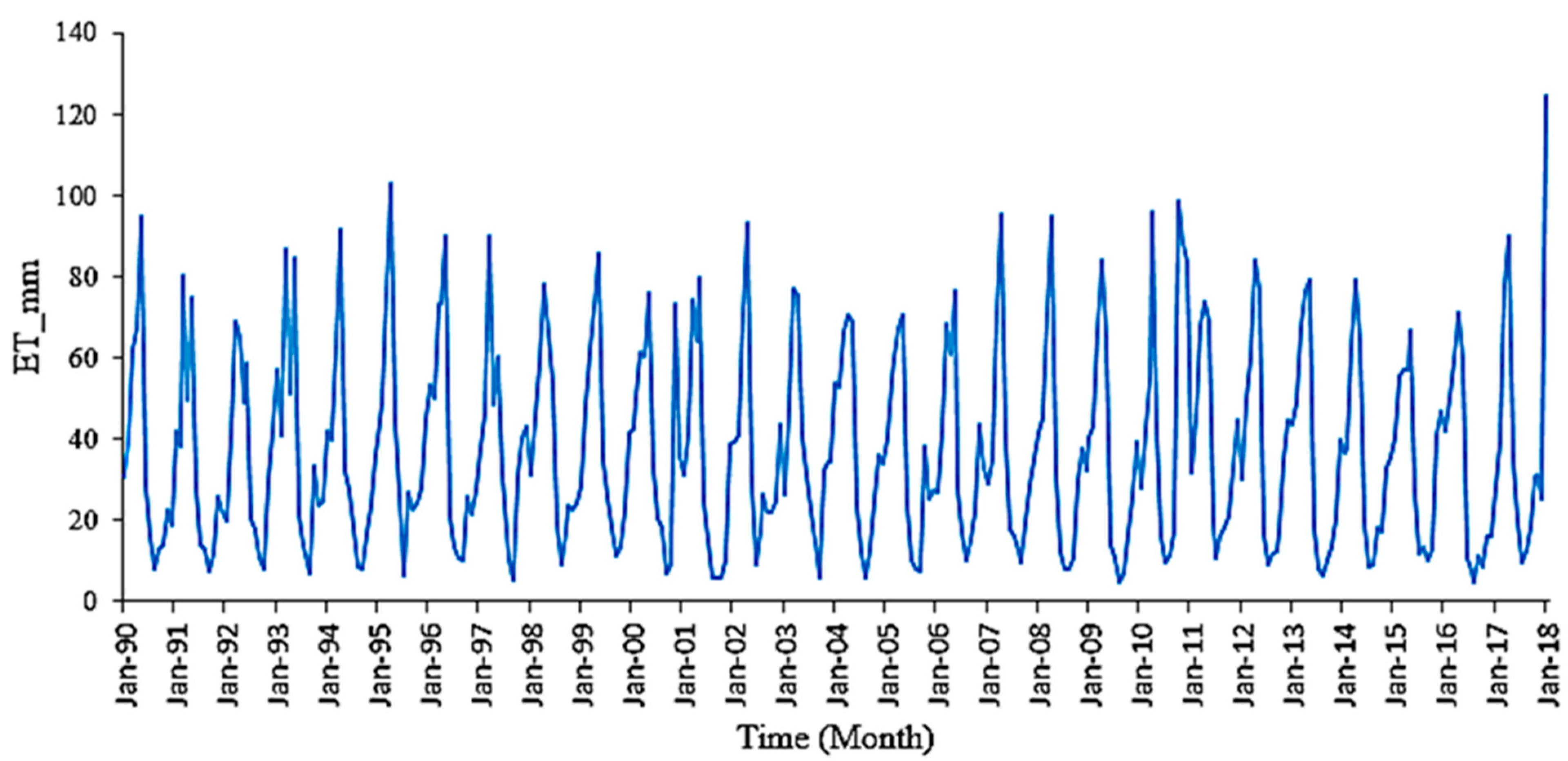
3.3.2. Simulated Evapotranspiration Trend (ET)

The SWAT-simulated results for ET show fluctuations from 1990, with a gradual increase in 2018 (Figure 10). From 1990 to 2018, the trends of ET increased by 29.71 mm, from 95.01 mm to 124.72 mm. This increase indicates the impact of LULC on ET, mainly resulting from the physical changes of the WRB land surface, which affects the efficiency of ET as a process (also see Figure 6 and Figure 10). Furthermore, Figure 11, which indicates the spatial distribution of ET in the basin, shows that ET in the far western areas is substantially lower than the eastern parts and towards the coastal areas of the WRB. This variation could be attributed to the bushland, which has expanded toward the coastal areas (Figure 6 and Figure 11). Similarly, the climatic conditions of the river basin, especially in the coastal and estuarine environments, are also likely to have contributed towards this variation. In general, the variation in ET, as shown in Figure 10, is largely consistent with previous studies, such as Wambura [83] who used a Moderate Resolution Imaging Spectroradiometer (MODIS) imagery program to study ET and potential evapotranspiration (PET) in the Ruvu sub-basin.

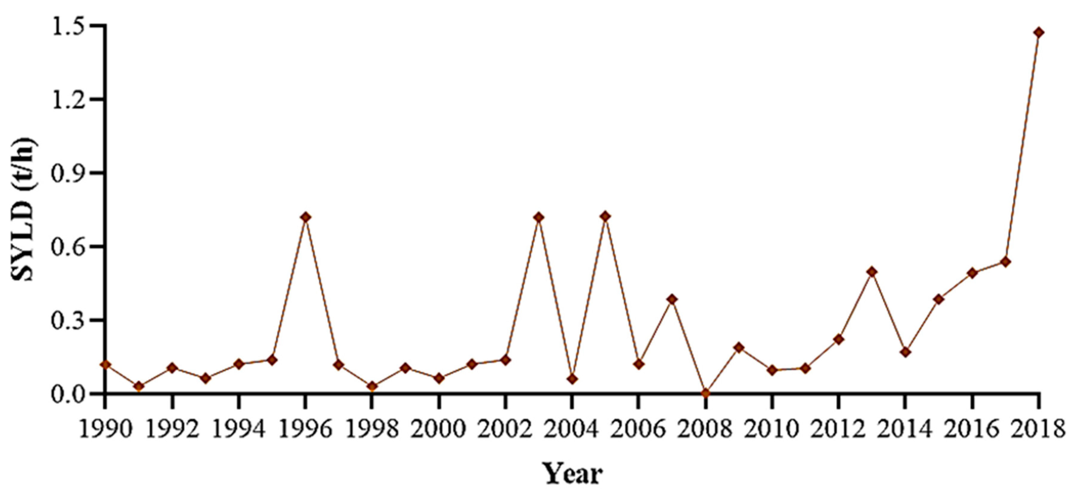
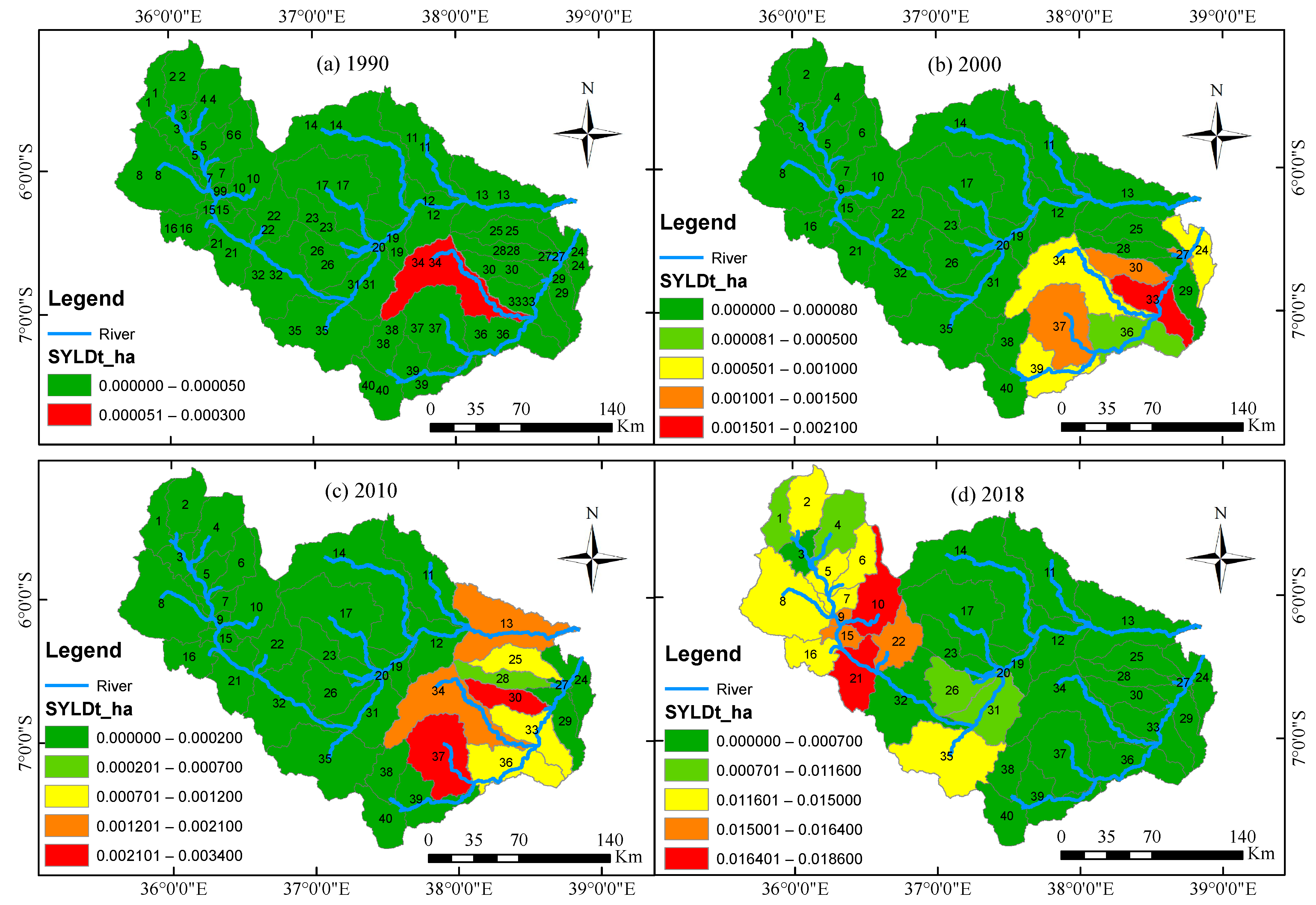
3.3.3. Spatio-Temporal Sediment Yield (SYLD) Distribution

Considerable changes in sediment yield in tons per hectare (SYLD t/h) occurred in the WRB from 1990 to 2018. The main change was a significant increase from 0.12 t/h to 1.5 t/h from 1990 to 2018 (Figure 12). Figure 13 shows the spatial distribution in the SYLD simulated from 1990 to 2018. In the starting year of the simulation, 1990, SYLD was more exposed in HRU 34 of the Ruvu sub-basin. In 2000, most SYLDs were imitated in HRUs 30, 33, and 37 of the same Ruvu sub-basin. In contrast, for the year 2010, the simulated results indicated that both sub-basins of the WRB were affected by the SYLD, with the Wami sub-basin being affected most at the downstream area (HRU 13). The Ruvu sub-basin affected both upstream and downstream, mostly in HRUs 30 and 37. Subsequently, for the last simulated year of 2018, the Wami sub-basin was the only area in the WRB affected by the SYLD, particularly in the upstream areas (HRUs 10 and 2). In general, the spatial distribution of the SYLD from 1990 to 2018 is characterised by notable features, such as in 1990, 2000, and 2010, where the Ruvu sub-basin was the only area simulated with the significant SYLD; in 2018, the situation changed to the Wami sub-basin, a situation that corresponds to the expansion of agricultural land cover (see Figure 6 and Figure 13 for comparison).

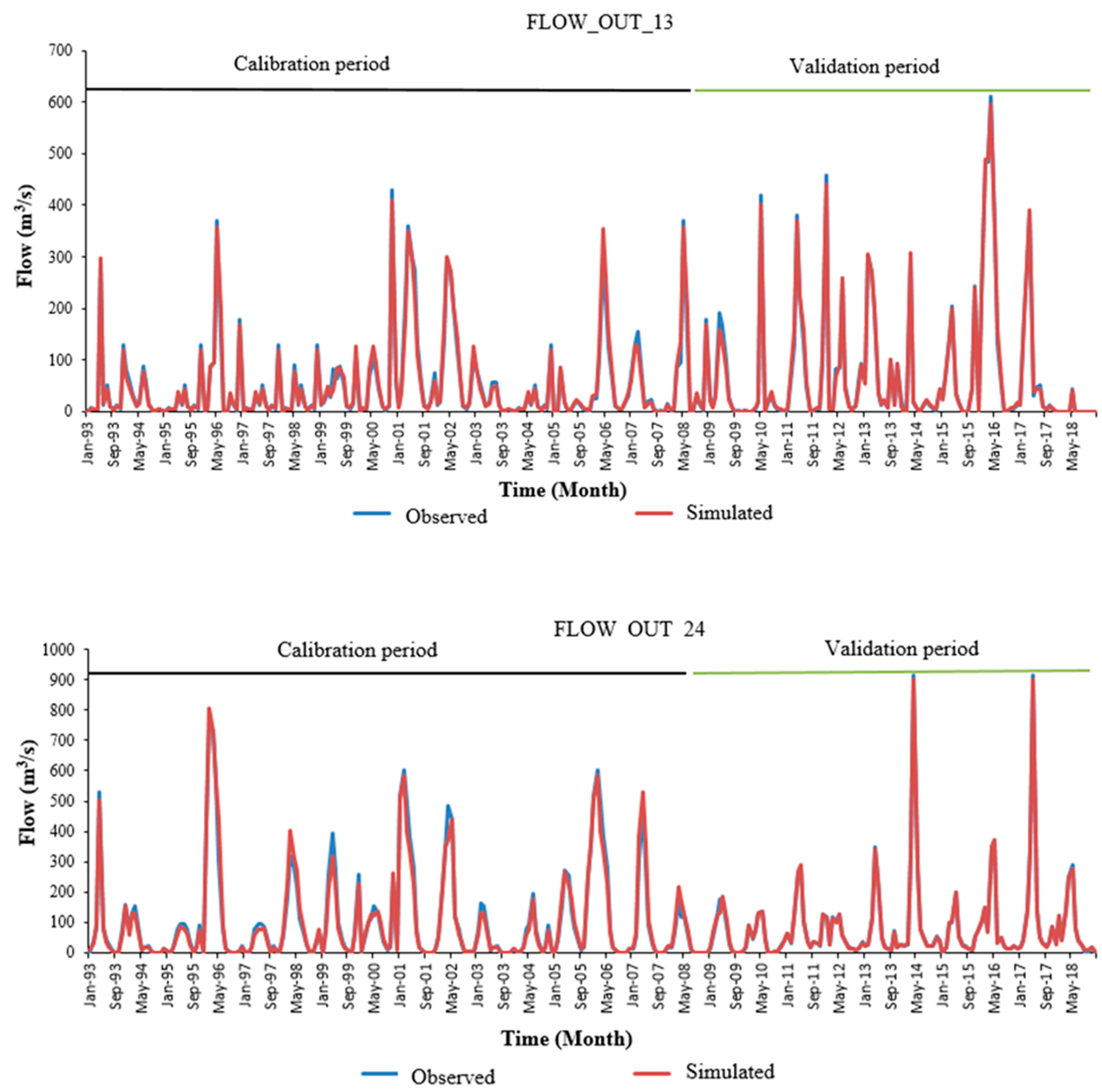
3.4. Calibration and Validation of the SWAT Model

According to [84], a hydrological model should be calibrated to estimate the model parameter values that provide the best possible hydrological results of interest. Hence, in this study, the SWAT model was calibrated using two gauging stations IG2 and 1H8 for FLOW_OUT_13 and FLOW_OUT_24. The calibration (1993–2008) and validation (2009–2018) were performed using the monthly flow data and the process started with a sensitivity analysis that identified seven key sensitive parameters governing the calibrated and validated outputs (

Table 10. The ranking of the seven most sensitive parameters and their final values.

Rank	Parameter	Parameter Description	Min Value	Max Value	SWAT Fitted Value
1	R_CN2.mgt	SCS runoff curve number	−0.3	0.3	−0.210000
2	SURLAG.bsn	Surface runoff lag time	5.54	14	8.501000
3	SOL.AWC.sol	Available water capacity of the soil layer	−0.8	0.8	0.550000
4	V_ALPHA-BF.gw	Baseflow alpha-factor	0	1.011	0.252750
5	V_GW-DELAY.gw	Groundwater delay	0	600	150.0000
6	GWQMN.gw	Threshold depth of water in the shallows Aquifer required for return flow to occur	0	2000	1700.000
7	ESCO.hru	Soil evaporation compensation factor	0	1	0.711777

). These parameters were manually adjusted iteratively to suit the satisfactory range before the auto-calibration was ran. The parameter ranges (minimum, maximum, and the fitted value) used for the model sensitivity analysis were found within the suggested ranges of the SWAT user’s manual and based on other studies, such as those conducted by [74,75]. Of the seven parameters, the four most sensitive parameters in our study were R_CN2.mgt, SURLAG.bsn, SOL.AWC.sol, and V_ALPHA-BF.gw.

Figure 14 shows the comparative results of the observed and simulated flows for the outlets FLOW_OUT_13 and /FLOW_OUT_24 of IG2 and 1H8 during the calibration (1993–2008) and validation periods (2009–2018). The graphical comparison between the observed and simulated annual river flow exhibits good agreement between the simulated and observed flows for both the calibration and validation periods (Figure 14).

Table 11. The model performance statistics for calibration and validation in the two outlets of the WRB.

Performance Periods	WRB Outlets	Average Monthly Flow (m3/s)		SWAT Evaluation Statistics
		Observed	Simulated	NSE	RSR	PBIAS
Calibration (Janaury 1993–December 2008)	FLOW_OUT_13	65.09	66.50	0.85	0.39	1.90
Validation (Janaury 2009–December 2018)	FLOW_OUT_13	70.84	71.26	0.83	0.37	1.70
Calibration (Janaury 1993–December 2008)	FLOW_OUT_24	109.96	110.72	0.68	0.49	1.40
Validation (Janaury 2009–December 2018)	FLOW_OUT_24	101.54	103.92	0.65	0.46	1.10

presents the statistical values that govern the SWAT-WRB model, the NSE, RSR, and PBIAS, which were found to be satisfactory for both the calibrated and simulated periods; these results also comply with others in the literature, such as in [79,80]. Therefore, our results indicate that the SWAT model performed well in simulating the hydrological conditions of the WRB.

4. Discussion

4.1. Impacts of LULCC on River Basin Hydrology over 29 Years (1990 to 2018)

LULC changes in the WRB have already been reported. The results for the studied years (1990, 2000, 2010, and 2018) on the different types of LULC indicate that most of the WRB natural areas, including forests and grasslands, were intensively converted into agricultural land from 1990 to 2018; further, these changes are anticipated to continue towards 2036 (Table 8). For example, agricultural land doubled from 10.6% in 1990 to 22.2% in 2018 and is predicted to continue to increase to 31.0% by 2036 (Table 6 and Table 8). Similarly, built-up areas increased between 1990 and 2018 (0.1% to 0.9%) and are expected to increase to 1.4% by 2036. Moreover, bushland increased from 16.7% in 1990 to 24.9% in 2018, despite a decrease in 2000, but is expected to increase to 27.1% by 2036. This land-use pattern reflects the influence of the population increase from 3.5 to 10 million people in the basin area from 1988 to 2018 [49]. This LULC pattern also highlights the common influence of economic forces that reinforce anthropogenic stimulus on LULC change in the river basin [85,86], and this is the main reason that the hydrological conditions of the wide-ranging river basins, including the WRB, have changed due to the transformation of natural vegetation, as substantiated by the SWAT hydrological model.

The observed LULC pattern is well established in the scientific literature—the deforestation of native vegetation influences several hydrological processes, resulting in changes in water and sediment yields [87], surface runoff [88], base and streamflow [33,89], river discharge [90], and latent heat fluxes to the hydrological cycle, including transpiration, interception loss, and evapotranspiration [91]. In the WRB, an increased conversion of the largest areas of natural vegetation into agriculture cover has played a great role in the increase in sediment yields generation from 0.12 t/h to 1.5 t/h, and the changes in WRB hydrological processes including WYLD, which decreased by 3.11 mm from 1990 to 2018. These results are in agreement with a previous study in the basin, particularly in the Wami sub-basin [41]. Spatially, the changes in WYLD and SYLD were consistent with the land-use pattern associated with agricultural expansion, which seems to intensively affect the western areas of the WRB, especially in recent years (Figure 15).

Other studies, including [92,93,94,95], have also noted similar LULC impacts on sediment loads. When sediments are eroded from their original places, some are deposited on the way while others continue to river basin streams [96]. Both transported and deposited sediments alter the basin’s hydrological components, such as the total WYLD, which was found to decrease in the WRB, particularly in the western part (Figure 14). Recalling statistically, the change in WYLD was observed from its components that indicated a decrease in groundwater flow with an increase in surface flow by 3.23 mm and 4.11 mm for Wami and Ruvu sub-basins, respectively (Table 9). The results suggest that the decrease of about 1,028,091 ha in forest cover within the basin area from 1990 to 2018 might also have caused a decrease in WYLD due to the decline in interception, which leads to more surface runoff in most cases. In addition, we associated the decrease in WYLD with the decrease in rainfall that was studied over the sub-basins of the WRB from 1990 to 2018 (Figure 8).

On the other hand, from the SWAT-simulated hydrograph for the observed and simulated water flow for both calibrated (1993–2008) and validated periods (2009–2018), the LULCC impacts that occurred from the 1990s to 2018 led to a decrease in annual flow, especially in 2018 (Figure 14). This is despite the good agreement between the simulated and observed discharges for both the calibration and validation periods, as revealed by the model performance statistics of FLOW_OUT_13 for the Wami sub-basin during calibration (NSE = 0.0.85, RSR = 0.39, PBIAS = 0.90) and validation (NSE = 0.83, RSR = 0.37, PBIAS = 1.70), and for the FLOW_OUT_24 for the Ruvu sub-basin during calibration (NSE = 0.68, RSR = 0.49, PBIAS = 1.40) and validation (NSE = 0.65, RSR = 0.46, PBIAS = 1.10). Furthermore, a comparison of the two hydrographs showed that the FLOW_OUT_13 for the Wami sub-basin had a lower flow (observed = 65.09 m³/s, simulated = 66.50 m³/s) than the FLOW_OUT_24 for the Ruvu sub-basin (observed = 109.96 m³/s, simulated = 110.72 m³/s), recorded during the calibration period (1993–2008). The same trend also occurred during the validation period (2009–2018), as shown in Table 11. Apart from the clear impacts of LULCCs associated with agriculture in the two sub-basins, the difference in the annual average flow observed in our study might have been caused by the difference in the climatic conditions of the two sub-basins: the semi-arid conditions of the far western areas of the FLOW_OUT_13 and the humidity and high rainfall of most areas covered by the FLOW_OUT_24. In addition, the high sensitivity of the R_CN2 parameter, which ranked first in the sensitivity analysis and governed the curve number of surface flow in the river basin (Table 10), could also contribute to the observed flow difference for the two sub-basin outlets. The high sensitivity of CN2 to streamflow has been reported in other studies, such as those conducted by Ndomba et al. [97], Mulungu and Munishi [98], Birhanu and Zemadim [99] in Tanzania river basins, and Baker and Miller [52] in East African watersheds.

Parallel to the sensitivity of the streamflow parameters and the LULCCs and their impacts on river flow, the rise and substantial variation in the spatial pattern of ET found in our study from 1990 to 2018 (Figure 10 and Figure 11) could be attributed to the same source. As noted in Figure 6 and Figure 11, the variation in ET seems to be mostly attributed to the increase in bushland. These results strongly agree with the SWAT model, which computes the ET based on the plant transpiration rate, maximum soil evaporation rate, and canopy water evaporation interception [74]. Moreover, as our study revealed an increase in temperature in the basin by 1 °C from 1990 to 2018, this could also be the reason for the observed increase in ET. Based on the comparison with the spatial LULC distribution (Figure 6 and Figure 11), the ET decreased more from the far west to the central and lower land areas. A study by FIU-GLOWS [46] reported similar findings of an increase in evaporative water loss in the lower streams of the WRB. It is worth noting that, as the lower land areas were also highly populated as indicated by the rapid increase in built-up areas (Figure 6), the increase in ET to the lower areas of the WRB might further lead to hydrological complications in the WRB rivers, tributaries, and reservoirs and affect the amount of water resources needed by the populations residing in those areas.

Therefore, based on the results of this study and those drawn from other research, including Wambura [42] and Wambura [35], it is clear that the LULC changes contributed to modifications in the basin land and hydrological parameters. The trends of the increase in all tested parameters signify the instability of the WRB hydrology. It is worth noting that the future trends of the modelled parameters depend on the good practice of the LULC in the river basin. For this reason, the researchers investigated and identified the land-use plan (LUP) currently being implemented in the basin (Appendix A, Figure A4) and predicted the LULC change of the river basin up to 2036 in order to determine the future of the LULC and its anticipated impacts on the identified hydrological parameters. In the first case, the existing LUP has six main land uses. In comparison with the current LULC of 2018, land-use with high hydrological effects (i.e., agriculture and built-up areas) is allocated more space (>50%). This implies that the current plan favours the hydrological instability of the WRB. The predicted LULC change up to 2036 is consistent with current patterns (Figure 7). The anticipated increase in agricultural land, bushland, and built-up areas and reduction in natural forest and water and wetlands follows the current LULC trend in the region; if this trend continues without remedial measures, its impacts on the hydrological components will increase considerably in the future, as simulated in our study. Furthermore, this will become more complicated with climate change, rapid population growth, and the need to achieve economic growth within the basin [49].

4.2. Hydrological Stability of the WRB

The SWAT results demonstrate that the LULC types considered in this study are significant and, therefore, important in affecting the hydrological components of the WRB. As statistically shown, the decrease in WYLD and the increase in SYLD and ET clearly define the instability of the WRB. On this basis, the detected changes in natural forests, built-up areas, and agricultural areas should be regulated in order to decrease the related impacts on the hydrological components and to obtain the hydrological stability of the basin. In this course, the land-use plan, which is in practice in the basin, is among the key areas for intervention since it has awarded a high priority to agricultural development. Generally, agriculture is one of the major income sources [45,95,100] and is supported with several strategies, such as Kilimo Kwanza (Agricultural First) and the Southern Agriculture corridor of Tanzania [101,102]. Such initiatives are implemented more in the arable lands of river basins, including the WRB [102]. Despite its significance, if not controlled by rationing as in the current LUP, its adverse impacts on basin hydrology are expected, as evidenced by the predicted LULC changes up to the year 2036.

Parallel to these observations, the specific hydrological response results showed that the far western areas of the WRB significantly reduced WYLD and increased SYLD. In contrast, the north-eastern and low-land areas also showed the same hydrological complexities due to indicators such as the rapid increase in built-up land and the significant increase in ET. Thus, to reverse this situation, our study proposes re-planning the river basin land-use and re-assessing the hydrologic changes to sustain the hydrological stability of the WRB. For the first case, we think that performing suitability analyses before allocating land-use could provide a better way of maintaining the hydrological conditions of the WRB. The latter should consider assessing the hydrological responses of the WRB using more parameters and with different models, including SWAT, in order to better understand the ecological conditions of the basin. Taken together, proper LUP and the regular monitoring of LULCCs and climatic factors are essential for the stability of the WRB.

5. Conclusions

This study assessed the impact of LULC changes on the hydrology of the WRB over 29 years (1990 to 2018) using SWAT in ArcGIS software and predicted its future trends using the CA–Markov model up to the year 2036. Landsat data were used to acquire land-use and land-cover changes and, together with hydro-meteorological, topological, and global soil data, to model the hydrology of the WRB. The substantial LULCCs are mainly due to the conversion of natural forests into agricultural areas. The rapid decrease in the forest areas, from 58.1% in 1990 to 42.7% in 2018, is primarily caused by the inefficient land-use plans drawing substantial land for agricultural use, which grew from 10.6% in 1990 to 22.2% in 2018 and is expected to increase to 31.0% by 2036. Parallel to these findings, the hydrological response to the LULC changes included a decrease in WYLD by 3.11 mm, an increase in ET by 29.71 mm, and an increase in SYLD from 0.12 t/h to 1.5 t/h, which define the hydrological instability of the WRB. Following this observation and examination of the causes, we advise possible mitigation measures that may be used to improve the current conditions of the river basin. Generally, the findings of this study provide baseline information for hydrologists, land-use planners, policymakers, resource managers, and decision-makers to elicit better planning and management decisions in the Wami–Ruvu Basin. Future studies should focus on investigating the hydrological conditions of the WRB by considering other key drivers of change besides LULCCs. They should be further extended to evaluate other hydrological parameters in order to better understand the hydrology of the WRB for the optimal use of water resources.

References

1. Mittal, N.; Bhave, A.G.; Mishra, A.; Singh, R. Impact of Human Intervention and Climate Change on Natural Flow Regime. Water Resour. Manag. 2016, 30, 685–699. [Google Scholar] [CrossRef] [Green Version]
2. Zhang, Y.; You, Q.; Chen, C.; Ge, J. Impacts of Climate Change on Streamflows under RCP scenarios: A Case study in Xin River Basin, China. Atmos. Res. 2016, 178–179, 521–534. [Google Scholar] [CrossRef]
3. Hu, M.; Sayama, T.; Duan, W.; Takara, K.; He, B.; Luo, P. Assessment of Hydrological Extremes in the Kamo River Basin, Japan. Hydrol. Sci. J. 2017, 62, 1255–1265. [Google Scholar] [CrossRef]
4. Aghsaei, H.; Mobarghaee Dinan, N.; Moridi, A.; Asadolahi, Z.; Delavar, M.; Fohrer, N.; Wagner, P.D. Effects of Dynamic Land Use/Land Cover Change on Water Resources and Sediment Yield in the Anzali Wetland Catchment, Gilan, Iran. Sci. Total Environ. 2020, 712, 136449. [Google Scholar] [CrossRef] [PubMed]
5. Anand, J.; Gosain, A.K.; Khosa, R. Prediction of Land Use Changes Based on Land Change Modeler and Attribution of Changes in the Water Balance of Ganga Basin to Land Use Change Using the SWAT Model. Sci. Total Environ. 2018, 644, 503–519. [Google Scholar] [CrossRef] [PubMed]
6. Tena, T.M.; Mwaanga, P.; Nguvulu, A. Impact of Land Use/Land Cover Change on Hydrological Components in Chongwe River Catchment. Sustainability 2019, 11, 6415. [Google Scholar] [CrossRef] [Green Version]
7. Huang, T.C.C.; Lo, K.F.A. Effects of Land Use Change on Sediment and Water Yields in Yang Ming Shan. Natl Parks, Taiwan. Environments 2015, 2, 32–42. [Google Scholar] [CrossRef] [Green Version]
8. Wang, G.; Zhang, Y.; Liu, G.; Chen, L. Impact of Land-Use Change on Hydrological Processes in the Maying River Basin, China. Sci. China Ser. D Earth Sci. 2006, 49, 1098–1110. [Google Scholar] [CrossRef]
9. Mutayoba, E.; Kashaigili, J.J.; Kahimba, F.C.; Mbungu, W.; Chilagane, N.A. Assessing the Impacts of Land Use and Land Cover Changes on Hydrology of the Mbarali River Sub-Catchment. The Case of Upper Great Ruaha Sub-Basin, Tanzania. Engineering 2018, 10, 616–635. [Google Scholar] [CrossRef] [Green Version]
10. Yang, W.; Long, D.; Bai, P. Impacts of Future Land Cover and Climate Changes on Runoff in the Mostly Afforested River Basin in North China. J. Hydrol. 2019, 570, 201–219. [Google Scholar] [CrossRef]
11. Wojkowski, J.; Młyński, D.; Lepeška, T.; Wałęga, A.; Radecki-Pawlik, A. Link between hydric potential and predictability of maximum flow for selected catchments in Western Carpathians. Sci. Total Environ. 2019, 683, 293–307. [Google Scholar] [CrossRef] [PubMed]
12. Zhang, Y.-W.; Shangguan, Z.-P. The Change of Soil Water Storage in Three Land Use Types after 10 Years on the Loess Plateau. Catena 2016, 147, 87–95. [Google Scholar] [CrossRef]
13. Pan, Y.; Gong, H.; Zhou, D.; Li, X.; Nakagoshi, N. Impact of Land Use Change on Groundwater Recharge in Guishui River Basin, China. Chin. Geogr. Sci. 2011, 21, 734–743. [Google Scholar] [CrossRef]
14. Younis, S.M.Z.; Ammar, A. Quantification of Impact of Changes in Land Use-Land Cover on Hydrology in the Upper Indus Basin, Pakistan. Egypt. J. Remote Sens. Space Sci. 2018, 21, 255–263. [Google Scholar] [CrossRef]
15. World Bank. World Development Indicators. Agricultural Inputs. 2017. Available online: http://wdi.worldbank.org/table/3.2 (accessed on 19 October 2021).
16. World Bank. World Development Indicators. Employment by Sector. 2017. Available online: http://wdi.worldbank.org/table/2.3 (accessed on 19 October 2021).
17. Tumbo, S.; Kahimba, F.; Mbilinyi, B.; Rwehumbiza, F.; Mahoo, H.F.; Mbungu, W.; Enfors, E. Impact of Projected Climate Change on Agricultural Production in Semi-Arid Areas of Tanzania: A Case of Same District. Afr. Crop Sci. J. 2012, 20, 453–463. [Google Scholar]
18. URT. Accelerating Pro-Poor Growth in the Context of Kilimo Kwanza; URT: Dar es Salaam, Tanzania, 2009; pp. 13–23. [Google Scholar]
19. Näschen, K.; Diekkrüger, B.; Evers, M.; Höllermann, B.; Steinbach, S.; Thonfeld, F. The Impact of Land Use/Land Cover Change (LULCC) on Water Resources in a Tropical Catchment in Tanzania under Different Climate Change Scenarios. Sustainability 2019, 11, 7083. [Google Scholar] [CrossRef] [Green Version]
20. Srivastava, A.; Kumari, N.; Maza, M. Hydrological Response to Agricultural Land Use Heterogeneity Using Variable Infiltration Capacity Model. Water Resour. Manag. 2020, 34, 3779–3794. [Google Scholar] [CrossRef]
21. Bessah, E.; Raji, A.O.; Taiwo, O.J.; Agodzo, S.K.; Ololade, O.O.; Strapasson, A. Hydrological Responses to Climate and Land Use Changes: The Paradox of Regional and Local Climate Effect in the Pra River Basin of Ghana. J. Hydrol. Reg. Stud. 2020, 27, 100654. [Google Scholar] [CrossRef]
22. Mbungu, W.B.; Kashaigili, J.J. Assessing the Hydrology of a Data-Scarce Tropical Watershed Using the Soil and Water Assessment Tool: Case of the Little Ruaha River Watershed in Iringa, Tanzania. Open J. Mod. Hydrol. 2017, 7, 65–89. [Google Scholar] [CrossRef] [Green Version]
23. Santos, V.; Laurent, F.; Abe, C.; Messner, F. Hydrologic Response to Land Use Change in a Large Basin in Eastern Amazon. Water 2018, 10, 429. [Google Scholar] [CrossRef] [Green Version]
24. Li, Z.; Liu, W.-Z.; Zhang, X.-C.; Zheng, F.-L. Impacts of Land Use Change and Climate Variability on Hydrology in an Agricultural Catchment on the Loess Plateau of China. J. Hydrol. 2009, 377, 35–42. [Google Scholar] [CrossRef]
25. Guzha, A.C.; Rufino, M.C.; Okoth, S.; Jacobs, S.; Nóbrega, R.L.B. Impacts of Land Use and Land Cover Change on Surface Runoff, Discharge and Low Flows: Evidence from East Africa. J. Hydrol. Reg. Stud. 2018, 15, 49–67. [Google Scholar] [CrossRef]
26. Pinto, L.; de Mello, C.; Owens, P.; Darrell, N.; Curi, N. Role of Inceptisols in the Hydrology of Mountainous Catchments in Southeastern Brazil. J. Hydrol. Eng. 2015, 21, 05015017. [Google Scholar] [CrossRef]
27. Bormann, H.; Elfert, S. Application of WaSiM-ETH Model to Northern German Lowland Catchments: Model Performance in Relation to Catchment Characteristics and Sensitivity to Land Use Change. Adv. Geosci. 2010, 27, 1–10. [Google Scholar] [CrossRef] [Green Version]
28. Golmohammadi, G.; Prasher, S.; Madani, A.; Rudra, R. Evaluating Three Hydrological Distributed Watershed Models: Mike-SHE, APEX, SWAT. Hydrology 2014, 1, 20–39. [Google Scholar] [CrossRef] [Green Version]
29. Neupane, R.P.; Kumar, S. Estimating the Effects of Potential Climate and Land Use Changes on Hydrologic Processes of a Large Agriculture Dominated Watershed. J. Hydrol. 2015, 529, 418–429. [Google Scholar] [CrossRef]
30. Zhang, J.; Ross, M. Hydrologic Modeling Impacts of Post-Mining Land Use Changes on Streamflow of Peace River, Florida. Chin. Geogr. Sci. 2015, 25, 728–738. [Google Scholar] [CrossRef] [Green Version]
31. Shivhare, N.; Dikshit, P.K.S.; Dwivedi, S.B. A Comparison of SWAT Model Calibration Techniques for Hydrological Modeling in the Ganga River Watershed. Engineering 2018, 4, 643–652. [Google Scholar] [CrossRef]
32. Leavesley, G.H.; Litchy, R.W.; Troutman, B.M.; Saindon, L.G. Precipitation-Runoff Modeling System: User’s Manual. In US Geological Survey Water Resources Investigative Report; U.S. Geological Survey, Water Resources Division: Reston, VA, USA, 1983. [Google Scholar] [CrossRef] [Green Version]
33. Aboelnour, M.A.; Engel, B.A.; Frisbee, M.D.; Gitau, M.W.; Flanagan, D.C. Impacts of Watershed Physical Properties and Land Use on Baseflow at Regional Scales. J. Hydrol. Reg. Stud. 2021, 35, 100810. [Google Scholar] [CrossRef]
34. Legesse, D.; Abiye, T.A.; Vallet-Coulomb, C.; Abate, H. Streamflow Sensitivity to Climate and Land Cover Changes: Meki River, Ethiopia. Hydrol. Earth Syst. Sci. 2010, 14, 2277–2287. [Google Scholar] [CrossRef] [Green Version]
35. Wambura, F.J.; Dietrich, O.; Lischeid, G. Improving a Distributed Hydrological Model Using Evapotranspiration-Related Boundary Conditions as Additional Constraints in a Data-Scarce River Basin. Hydrol. Processes 2018, 32, 759–775. [Google Scholar] [CrossRef]
36. Nie, W.; Yuan, Y.; Kepner, W.; Nash, M.S.; Jackson, M.; Erickson, C. Assessing Impacts of Landuse and Landcover Changes on Hydrology for the Upper San Pedro Watershed. J. Hydrol. 2011, 407, 105–114. [Google Scholar] [CrossRef]
37. Zhu, C.; Li, Y. Long-Term Hydrological Impacts of Land Use/Land Cover Change from 1984 to 2010 in the Little River Watershed, Tennessee. Int. Soil Water Conserv. Res. 2014, 2, 11–21. [Google Scholar] [CrossRef] [Green Version]
38. Gashaw, T.; Tulu, T.; Argaw, M.; Worqlul, A.W. Modeling the Hydrological Impacts of Land Use/Land Cover Changes in the Andassa Watershed, Blue Nile Basin, Ethiopia. Sci. Total Environ. 2018, 619–620, 1394–1408. [Google Scholar] [CrossRef] [PubMed]
39. Wang, Q.; Xu, Y.; Wang, Y.; Zhang, Y.; Xiang, J.; Xu, Y.; Wang, J. Individual and Combined Impacts of Future Land-Use and Climate Conditions on Extreme Hydrological Events in a Representative Basin of the Yangtze River Delta, China. Atmos. Res. 2020, 236, 104805. [Google Scholar] [CrossRef]
40. Zhang, H.; Wang, B.; Liu, D.L.; Zhang, M.; Leslie, L.M.; Yu, Q. Using an Improved SWAT Model to Simulate Hydrological Responses to Land Use Change: A Case Study of a Catchment in Tropical Australia. J. Hydrol. 2020, 585, 124822. [Google Scholar] [CrossRef]
41. Nobert, J.; Jeremiah, J. Hydrological Response of Watershed Systems to Land Use/Cover Change. A Case of Wami River Basin. Open Hydrol. J. 2012, 6, 78–87. [Google Scholar] [CrossRef]
42. Wambura, F. Stream Flow Response to Skilled and Non-Linear Bias Corrected GCM Precipitation Change in the Wami River Sub-Basin, Tanzania. Br. J. Environ. Clim. Change 2014, 4, 389–408. [Google Scholar] [CrossRef]
43. Natkhin, M.; Dietrich, O.; Schäfer, M.P.; Lischeid, G. The Effects of Climate and Changing Land Use on the Discharge Regime of a Small Catchment in Tanzania. Reg. Environ. Change 2015, 15, 1269–1280. [Google Scholar] [CrossRef]
44. Aziz, N.; Minallah, N.; Junaid, A.; Gul, K. Performance analysis of artificial neural network based land cover classification. Int. J. Mar. Environ. Sci. 2017, 11, 422. [Google Scholar]
45. IUCN. IUCN Eastern and Southern Africa Programme. In The Ruvu Basin: A Situation Analysis; IUCN—ESARO Publications Service Unit: Nairobi, Kenya, 2010. [Google Scholar]
46. FIU-GLOWS, Water Atlas of the Wami/Ruvu Basin, Tanzania. 2014. Available online: http://dpanther.fiu.edu/sobek/FIGW000010/00001 (accessed on 20 September 2021).
47. Kashaigili, J.J. Rapid Environmental Flow Assessment for the Ruvu River, A Consultancy Report submitted to iWASH, 2011. Available online: http://www.suaire.sua.ac.tz/bitstream/handle/123456789/1481/Kashaigili17.pdf (accessed on 18 November 2021).
48. WRBWO. Wami/Ruvu Basin Annual Hydrological Report; WRB-Water Office: Morogoro, Tanzania, 2008.
49. Ngondo, J.; Mango, J.; Liu, R.; Nobert, J.; Dubi, A.; Cheng, H. Land-Use and Land-Cover (LULC) Change Detection and the Implications for Coastal Water Resource Management in the Wami–Ruvu Basin, Tanzania. Sustainability 2021, 13, 4092. [Google Scholar] [CrossRef]
50. JICA. The Study on Water Resources Management and Development in Wami/Ruvu Basin in the United Republic of Tanzania. 2013. Available online: https://www.jica.go.jp/tanzania/english/index.html (accessed on 17 August 2021).
51. Arnold, J.G.; Srinivasan, R.; Muttiah, R.S.; Williams, J.R. Large Area Hydrologic Modeling and Assessment Part I: Model. Development1. JAWRA J. Am. Water Resour. Assoc. 1998, 34, 73–89. [Google Scholar] [CrossRef]
52. Baker, T.J.; Miller, S.N. Using the Soil and Water Assessment Tool (SWAT) to Assess Land Use Impact on Water Resources in an East African Watershed. J. Hydrol. 2013, 486, 100–111. [Google Scholar] [CrossRef]
53. TAMU. 2021. Available online: https://swat.tamu.edu/ (accessed on 10 May 2021).
54. ALOSW3D. Digital Elevation Model. 2021. Available online: https://www.eorc.jaxa.jp/ALOS/en/aw3d30/data/index.htm (accessed on 10 May 2021).
55. Florinsky, I.V.; Skrypitsyna, T.N.; Luschikova, O.S. Comparative Accuracy of the AW3D30 DSM, ASTER GDEM, and SRTM1 DEM: A Case Study on the Zaoksky Testing Ground, Central European Russia. Remote Sens. Lett. 2018, 9, 706–714. [Google Scholar] [CrossRef]
56. Purinton, B.; Bookhagen, B. Validation of Digital Elevation Models (DEMs) and Comparison of Geomorphic Metrics on the Southern Central Andean Plateau. Earth Surf. Dynam. 2017, 5, 211–237. [Google Scholar] [CrossRef] [Green Version]
57. Santillan, J.; Makinano-Santillan, M. Vertical Accuracy Assessment of 30-m Resolution Alos, Aster, AND SRTM Global DEMS over Northeastern Mindanao, Philippines. Int. Arch. Photogramm. Remote Sens. Spat. Inf. Sci. 2016, XLI, 149–156. [Google Scholar] [CrossRef] [Green Version]
58. Yap, L.; Kandé, L.H.; Nouayou, R.; Kamguia, J.; Ngouh, N.A.; Makuate, M.B. Vertical Accuracy Evaluation of Freely Available Latest High-Resolution (30 m) Global Digital Elevation Models over Cameroon (Central Africa) with GPS/Leveling Ground Control Points. Int. J. Digit. Earth 2019, 12, 500–524. [Google Scholar] [CrossRef]
59. FAO. Digital Soil Map of the World. 2021. Available online: http://www.fao.org/geonetwork/srv/en/metadata.show%3Fid=14116 (accessed on 11 September 2020).
60. Dahal, P.; Shrestha, M.L.; Panthi, J.; Pradhananga, D. Modeling the future impacts of climate change on water availability in the Karnali River Basin of Nepal Himalaya. Environ. Res. 2020, 185, 109430. [Google Scholar] [CrossRef]
61. Aredehey, G.; Mezgebu, A.; Girma, A. The effects of land use land cover change on hydrological flow in Giba catchment, Tigray, Ethiopia. Cogent Environ. Sci. 2020, 6, 1785780. [Google Scholar] [CrossRef]
62. Wambura, F.J.; Dietrich, O.; Lischeid, G. Evaluation of Spatio-Temporal Patterns of Remotely Sensed Evapotranspiration to Infer Information about Hydrological Behaviour in a Data-Scarce Region. Water 2017, 9, 333. [Google Scholar] [CrossRef] [Green Version]
63. USGS. Global Geographacal Datasets. 2020. Available online: https://glovis.usgs.gov (accessed on 18 October 2020).
64. Bishop, C.M. Neural Networks for Pattern Recognition; Oxford University Press: New York, NY, USA, 1995. [Google Scholar]
65. Tilahun, A.; Bogale, T. Accuracy Assessment of Land Use Land Cover Classification Using Google Earth. Am. J. Environ. Prot. 2015, 4, 193–198. [Google Scholar] [CrossRef]
66. Rwanga, S.S.; Ndambuki, J.M. Accuracy Assessment of Land Use/Land Cover Classification Using Remote Sensing and GIS. Int. J. Geosci. 2017, 8, 611–622. [Google Scholar] [CrossRef] [Green Version]
67. Palmate, S.S.; Pandey, A.; Mishra, S.K. Modelling Spatiotemporal Land Dynamics for a Trans-Boundary River Basin Using Integrated Cellular Automata and Markov Chain Approach. Appl. Geogr. 2017, 82, 11–23. [Google Scholar] [CrossRef]
68. de Oliveira Barros, K.; Alvares Soares Ribeiro, C.A.; Marcatti, G.E.; Lorenzon, A.S.; Martins de Castro, N.L.; Domingues, G.F.; Romário de Carvalho, J.; Rosa dos Santos, A. Markov Chains and Cellular Automata to Predict Environments Subject to Desertification. J. Environ. Manag. 2018, 225, 160–167. [Google Scholar] [CrossRef]
69. Guan, D.; Li, H.; Inohae, T.; Su, W.; Nagaie, T.; Hokao, K. Modeling Urban Land Use Change by the Integration of Cellular Automaton and Markov Model. Ecol. Modell. 2011, 222, 3761–3772. [Google Scholar] [CrossRef]
70. Wambura, F.J.; Ndomba, P.M.; Kongo, V.; Tumbo, S.D. Uncertainty of Runoff Projections under Changing Climate in Wami River Sub-Basin. J. Hydrol. Reg. Stud. 2015, 4, 333–348. [Google Scholar] [CrossRef] [Green Version]
71. Abbaspour, K.C.; Vaghefi, S.A.; Srinivasan, R. A Guideline for Successful Calibration and Uncertainty Analysis for Soil and Water Assessment: A Review of Papers from the 2016 International SWAT Conference. Water 2018, 10, 6. [Google Scholar] [CrossRef] [Green Version]
72. Winchell, M.R.; Srinivasan, M.D.; Arnold, J.; Arc, S.W.A.T. Interface for SWAT 2005–Users’ Guide. Blackland Research Center, Texas Agricultural Experiment Station and Grassland, Soil and Water Research Laboratory; United States Department of Agriculture Agricultural Research Service: Temple, TX, USA, 2007. [Google Scholar]
73. Abbaspour, K.C.; Yang, J.; Maximov, I.; Siber, R.; Bogner, K.; Mieleitner, J.; Zobrist, J.; Srinivasan, R. Modelling Hydrology and Water Quality in the Pre-Alpine/Alpine Thur Watershed Using SWAT. J. Hydrol. 2007, 333, 413–430. [Google Scholar] [CrossRef]
74. Neitsch, S.L.; Arnold, J.G.; Kiniry, J.R.; Williams, J.R. Soil and Water Assessment Tool Theoretical Documentation, version 2009. In Texas Water Resources Institute Technical Report No. 406; Texas A&M University: College Station, TX, USA, 2011; Volume 2009. [Google Scholar]
75. Twisa, S.; Kazumba, S.; Kurian, M.; Buchroithner, M.F. Evaluating and Predicting the Effects of Land Use Changes on Hydrology in Wami River Basin, Tanzania. Hydrology 2020, 7, 17. [Google Scholar] [CrossRef] [Green Version]
76. Arnold, J.G.; Moriasi, D.N.; Gassman, P.W.; Abbaspour, K.C.; White, M.J.; Srinivasan, R.; Santhi, C.; Harmel, R.D.; van Griensven, A.; Van Liew, M.W.; et al. SWAT: Model Use, Calibration, and Validation. Trans. ASABE 2012, 55, 1491–1508. [Google Scholar] [CrossRef]
77. Abbaspour, K.C.; Johnson, C.A.; van Genuchten, M.T. Estimating Uncertain Flow and Transport Parameters Using a Sequential Uncertainty Fitting Procedure. Vadose Zone J. 2004, 3, 1340–1352. [Google Scholar] [CrossRef]
78. Nash, J.E.; Sutcliffe, J.V. River Flow Forecasting through Conceptual Models Part I—A Discussion of Principles. J. Hydrol. 1970, 10, 282–290. [Google Scholar] [CrossRef]
79. Moriasi, D.; Arnold, J.; Van Liew, M.; Bingner, R.; Harmel, R.D.; Veith, T. Model Evaluation Guidelines for Systematic Quantification of Accuracy in Watershed Simulations. Trans. ASABE 2007, 50, 885–900. [Google Scholar] [CrossRef]
80. Moriasi, D.; Gitau, M.; Pai, N.; Daggupati, P. Hydrologic and Water Quality Models: Performance Measures and Evaluation Criteria. Trans. ASABE (Am. Soc. Agric. Biol. Eng.) 2015, 58, 1763–1785. [Google Scholar]
81. Twisa, S.; Buchroithner, M.F. Land-Use and Land-Cover (LULC) Change Detection in Wami River Basin, Tanzania. Land 2019, 8, 136. [Google Scholar] [CrossRef] [Green Version]
82. Arnold, J.G.; Kiniry, J.R.; Srinivasan, R.; Williams, J.R.; Haney, E.B.; Neitsch, S.L. Soil and Water Assessment Tool Input-Output File Documentation. Soil and Water Research Laboratory, Agricultural Research Service, Grassland, 808 East Black Land Road, Temple, Texas. 2011. Available online: https://swat.tamu.edu/media/19754/swat-io-2009.pdf (accessed on 14 November 2021).
83. Wambura, F.J. Sensitivity of the Evapotranspiration Deficit Index to Its Parameters and Different Temporal Scales. Hydrology 2021, 8, 26. [Google Scholar] [CrossRef]
84. Huang, S.; Shah, H.; Naz, B.S.; Shrestha, N.; Mishra, V.; Daggupati, P.; Ghimire, U.; Vetter, T. Impacts of hydrological model calibration on projected hydrological changes under climate change—a multi-model assessment in three large river basins. Clim. Change 2020, 163, 1143–1164. [Google Scholar] [CrossRef]
85. Wang, X.; Zheng, D.; Shen, Y. Land Use Change and Its Driving Forces on the Tibetan Plateau During 1990–2000. Catena 2008, 72, 56–66. [Google Scholar] [CrossRef]
86. Butt, A.; Shabbir, R.; Ahmad, S.S.; Aziz, N. Land Use Change Mapping and Analysis Using Remote Sensing and GIS: A Case Study of Simly Watershed, Islamabad, Pakistan. Egypt. J. Remote Sens. Space Sci. 2015, 18, 251–259. [Google Scholar] [CrossRef] [Green Version]
87. Mendonça dos Santos, F.; Proença de Oliveira, R.; Augusto Di Lollo, J. Effects of Land Use Changes on Streamflow and Sediment Yield in Atibaia River Basin—SP, Brazil. Water 2020, 12, 1711. [Google Scholar] [CrossRef]
88. Wang, F.; Ge, Q.; Yu, Q.; Wang, H.; Xu, X. Impacts of Land-Use and Land-Cover Changes on River Runoff in Yellow River Basin for Period of 1956–2012. Chin. Geogr. Sci. 2017, 27, 13–24. [Google Scholar] [CrossRef] [Green Version]
89. Zhang, Y.-K.; Schilling, K.E. Increasing Streamflow and Baseflow in Mississippi River since the 1940s: Effect of Land Use Change. J. Hydrol. 2006, 324, 412–422. [Google Scholar] [CrossRef]
90. Costa, M.H.; Botta, A.; Cardille, J.A. Effects of Large-Scale Changes in Land Cover on the Discharge of the Tocantins River, Southeastern Amazonia. J. Hydrol. 2003, 283, 206–217. [Google Scholar] [CrossRef]
91. Kim, W.; Kanae, S.; Agata, Y.; Oki, T. Simulation of Potential Impacts of Land Use/Cover Changes on Surface Water Fluxes in the Chaophraya River Basin, Thailand. J. Geophys. Res. 2005, 110. [Google Scholar] [CrossRef] [Green Version]
92. Ngoye, E.; Machiwa, J.F. The Influence of Land-Use Patterns in the Ruvu River Watershed on Water Quality in the River System. Phys. Chem. Earth Parts A B C 2004, 29, 1161–1166. [Google Scholar] [CrossRef]
93. Yanda, P.Z.; Munishi, P. Hydrologic and Land Use/Cover Change Analysis for the Ruvu River (Uluguru) and Sigi River (East Usambara) Watersheds. For WWF/CARE Dar es Salaam; Tanzania. 2007. Available online: https://scholar.google.com/scholar?hl=en&as_sdt=0%2C5&q=Hydrologic+and+Land+Use%2FCover+Change+Analysis+for+the+Ruvu+River+%28Uluguru%29+and+Sigi+River+%28East+Usambara%29+Watersheds&btnG= (accessed on 19 August 2021).
94. Msaghaa, J.J.; Melesse, A.M.; Ndomba, P.M. Modeling Sediment Dynamics: Effect of Land Use, Topography, and Land Management in the Wami-Ruvu Basin, Tanzania. In Nile River Basin:Ecohydrological Challenges, Climate Change and Hydropolitics; Melesse, A.M., Abtew, W., Setegn, S.G., Eds.; Springer International Publishing: Cham, Switzerland, 2014; pp. 165–192. [Google Scholar]
95. Mbungu, W.B. Impacts of Land Use and Land Cover Changes, and Climate Variability on Hydrology and Soil Erosion in the Upper Ruvu Watershed, Tanzania [Diss.]; Virginia Tech: Blacksburg, Virginia, 2017. [Google Scholar]
96. Gao, P.; Puckett, J. A New Approach for Linking Event-Based Upland Sediment Sources to Downstream Suspended Sediment Transport. Earth Surf. Processes Landf. 2012, 37, 169–179. [Google Scholar] [CrossRef]
97. Ndomba, P.; Mtalo, F.; Killingtveit, A. SWAT Model Application in a Data Scarce Tropical Complex Catchment in Tanzania. Phys. Chem. Earth Parts A B C 2008, 33, 626–632. [Google Scholar] [CrossRef]
98. Mulungu, D.M.M.; Munishi, S.E. Simiyu River Catchment Parameterization Using SWAT Model. Phys. Chem. Earth Parts A B C 2007, 32, 1032–1039. [Google Scholar] [CrossRef]
99. Birhanu, Z.; Zemadim, B. Hydrological Modeling of the Kihansi River Catchment in South Central, Tanzania Using SWAT Model. Water Resour. Environ. Eng. 2009, 1, 001–010. [Google Scholar]
100. Lopa, D.; Mwanyoka, I.; Jambiya, G.; Massoud, T.; Harrison, P.; Ellis-Jones, M.; Blomley, T.; Leimona, B.; van Noordwijk, M.; Burgess, N.D. Towards Operational Payments for Water Ecosystem Services in Tanzania: A Case Study from the Uluguru Mountains. Oryx 2012, 46, 34–44. [Google Scholar] [CrossRef] [Green Version]
101. URT. The Kilimo Kwanza Resolution; URT: Dar es Salaam, Tanzania, 2009. [Google Scholar]
102. Seeteram, N.A.; Hyera, P.T.; Kaaya, L.T.; Lalika, M.C.S.; Anderson, E.P. Conserving Rivers and Their Biodiversity in Tanzania. Water 2019, 11, 2612. [Google Scholar] [CrossRef] [Green Version]
Figure 1. The location of the study area: the Wami-Ruvu Basin (WRB), Tanzania.
Water 14 00184 g001
Figure 2. The topography and soil data used for the modelling of the Wami–Ruvu Basin.
Water 14 00184 g002
Figure 3. The LULC data of the WRB used for the SWAT model: (a) Classification according to the ANN technique; (b) Reclassified based on the SWAT land-use database.
Water 14 00184 g003
Figure 4. A flowchart describing the data processing.
Water 14 00184 g004
Figure 5. The delineated stream and sub-stream networks of the Wami–Ruvu Basin, Tanzania.
Water 14 00184 g005
Figure 6. The classified LULC types of the Wami–Ruvu Basin for 1990, 2000, 2010, and 2018.
Water 14 00184 g006
Figure 7. The LULC maps of the Wami–Ruvu Basin, (a) for 2018 and (b) projected by the CA–Markov model for the year 2036.
Water 14 00184 g007
Figure 8. (a) The annual precipitation and (b) the annual temperature for the sub-basins of the WRB.
Water 14 00184 g008
Figure 9. The spatial WYLD distribution in the WRB for (a) 1900, (b) 2000, (c) 2010, and (d) 2018. Note: The numbers 1–40 are sub-catchments from the delineation process.
Water 14 00184 g009
Figure 10. The temporal trends of simulated ET in the WRB.
Water 14 00184 g010
Figure 11. The simulated spatial pattern of ET in the WRB for the years (a) 1990, (b) 2000, (c) 2010, and (d) 2018.
Water 14 00184 g011
Figure 12. The temporal trends of SYLD simulated in the WRB.
Water 14 00184 g012
Figure 13. The simulated spatial pattern of SYLD in the WRB for the years (a) 1990, (b) 2000, (c) 2010 and (d) 2018.
Water 14 00184 g013
Figure 14. The hydrographs of the observed and simulated monthly water flow for the calibration and validation periods.
Water 14 00184 g014
Figure 15. (a) The LULC distribution and its associated impacts on (b) SYLD and (c) WYLD in 2018.
Water 14 00184 g015