
Inter-Annual and Seasonal Variability of Flows: Delivering Climate-Smart Environmental Flow Reference Values


Abstract
:
1. Introduction
2. Materials and Methods
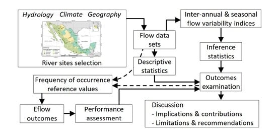
2.1. Research Design
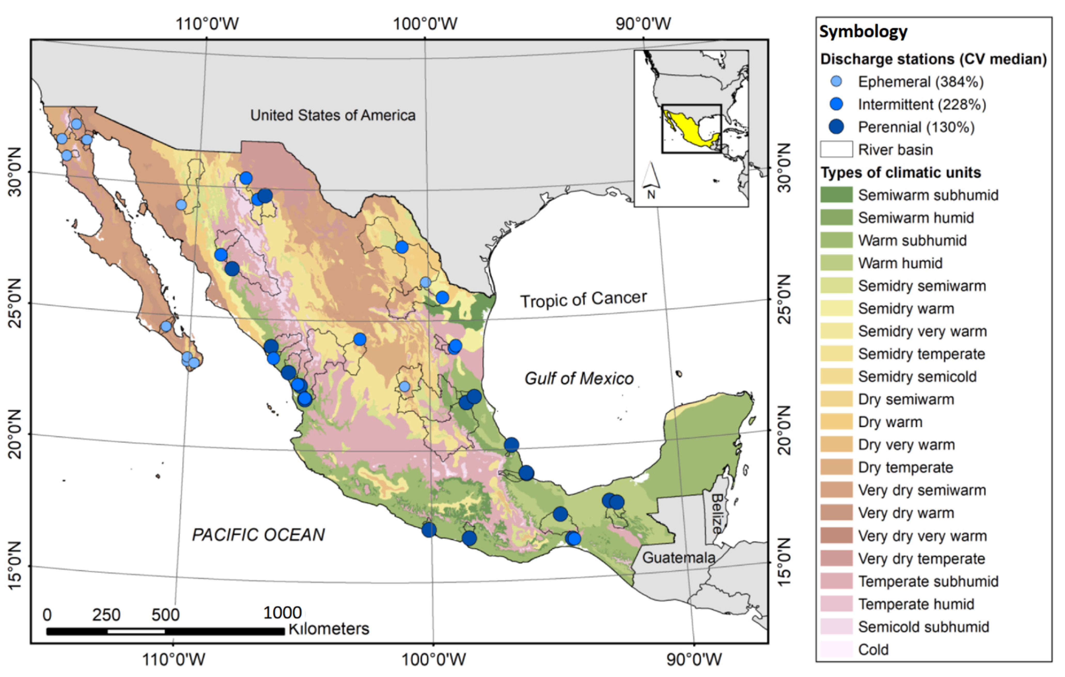
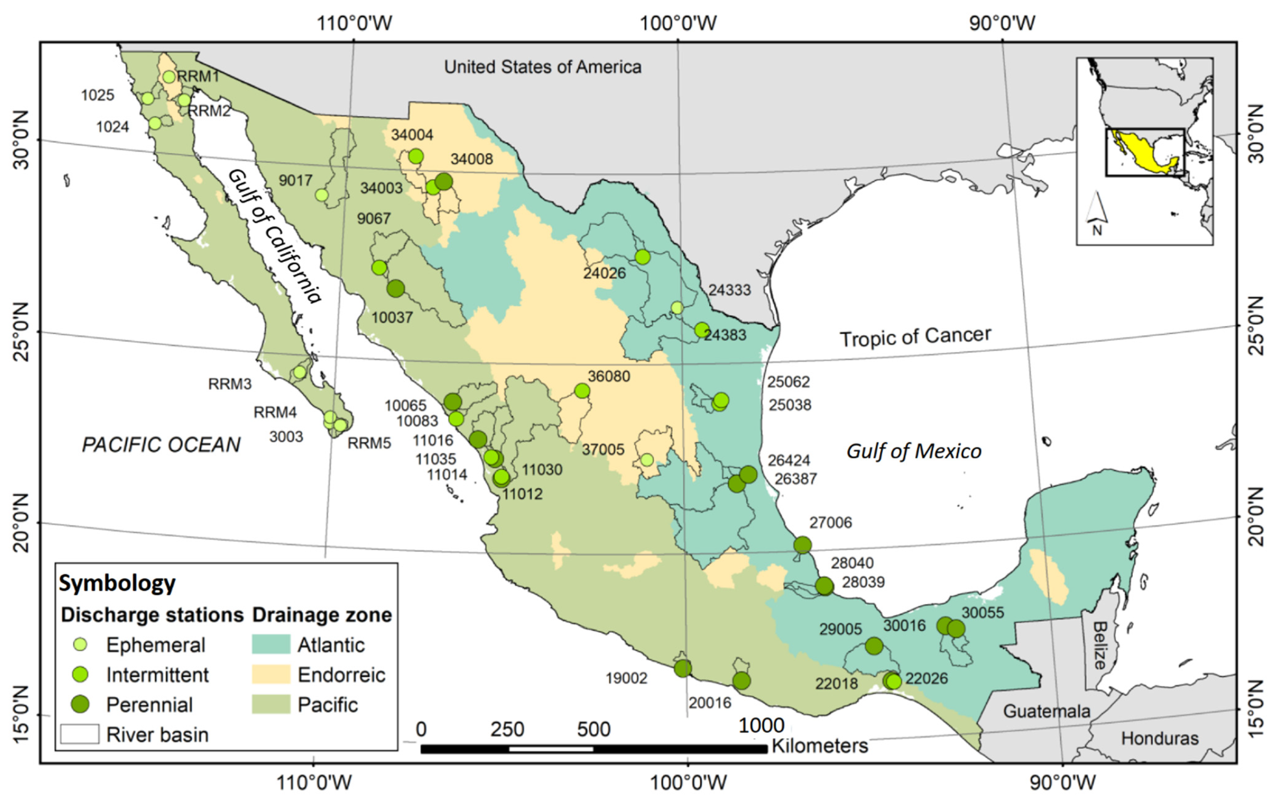
2.1.1. River Basin Selection
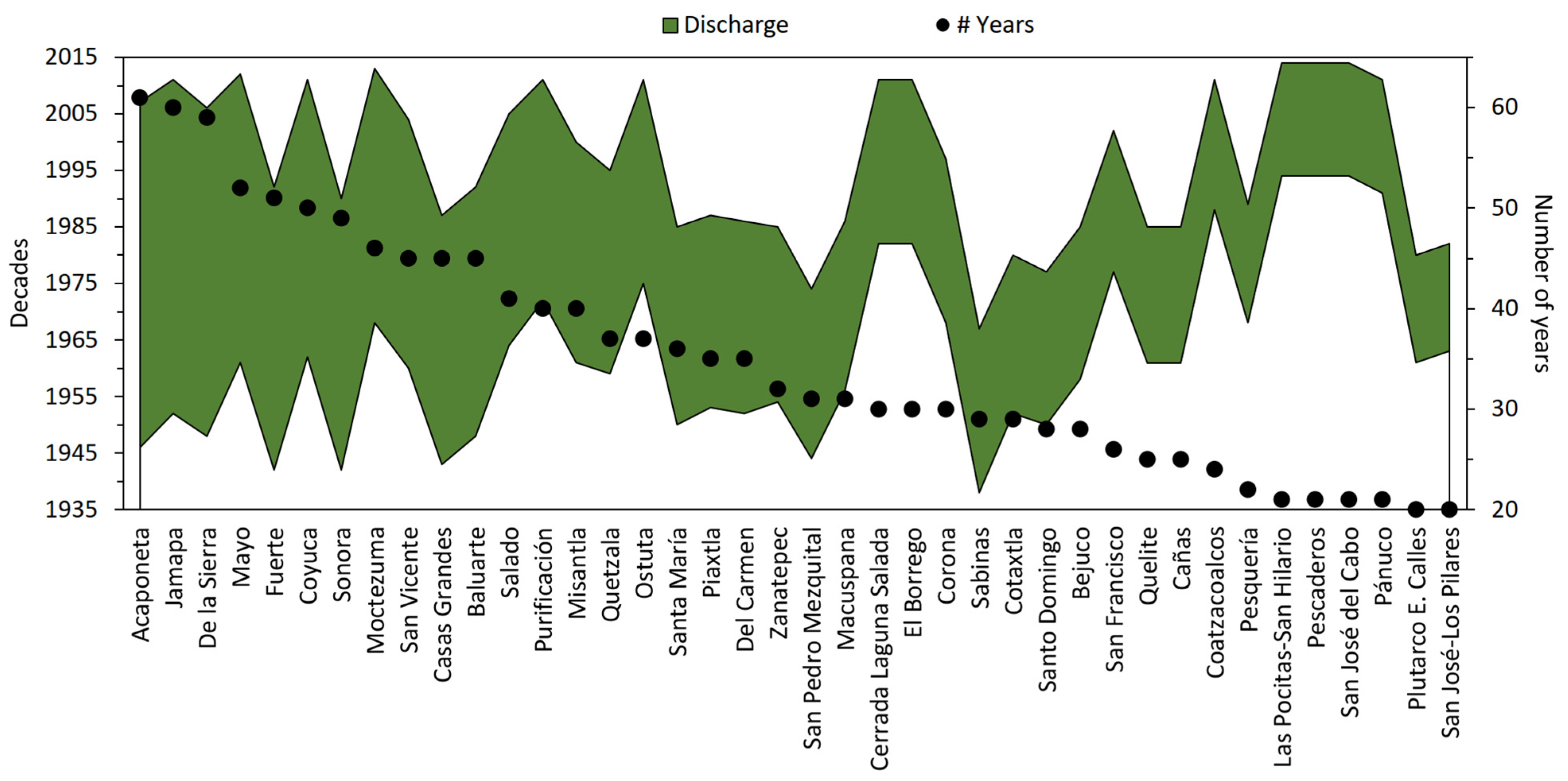
2.1.2. Data Type, Source, and Requirements
2.1.3. Analysis Techniques: Indices, Descriptive and Inference Statistics
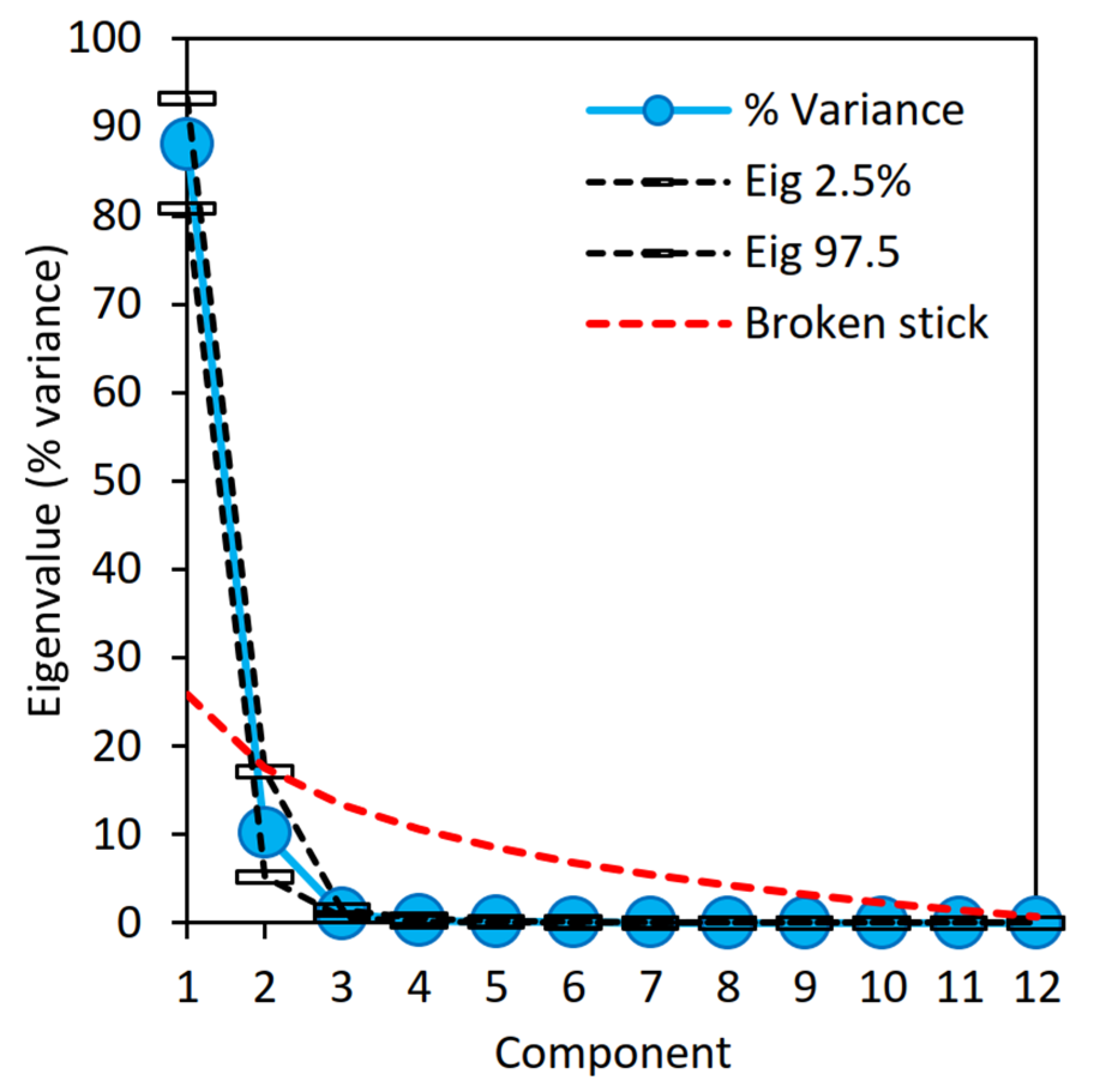
- The correlation of PC1 (significant variance p-value < 0.05) with independent indices of hydrological variability, in line with the previous studies [22,23,24]. The indices considered were the coefficient of variation (CV) and the baseflow (BFI), the former an indication of long-term variability between seasons, while the latter is representative of short-term variability [7]. Coefficients of determination were calculated according to polynomic regressions (R2) of the PC1 by CV and BFI for the whole population and based on linear regressions (r2) for each streamflow class. Additionally, the CV and BFI medians, ±1 quartile, and full range are provided.
2.2. Reference Values for Climate-Smart Environmental Flows and Water Reserves
2.3. Performance Assessment of the Reserves for Environmental Water Allocation
3. Results
3.1. Hydrological Contributions per Streamflow Type: Characteristics and Relationships
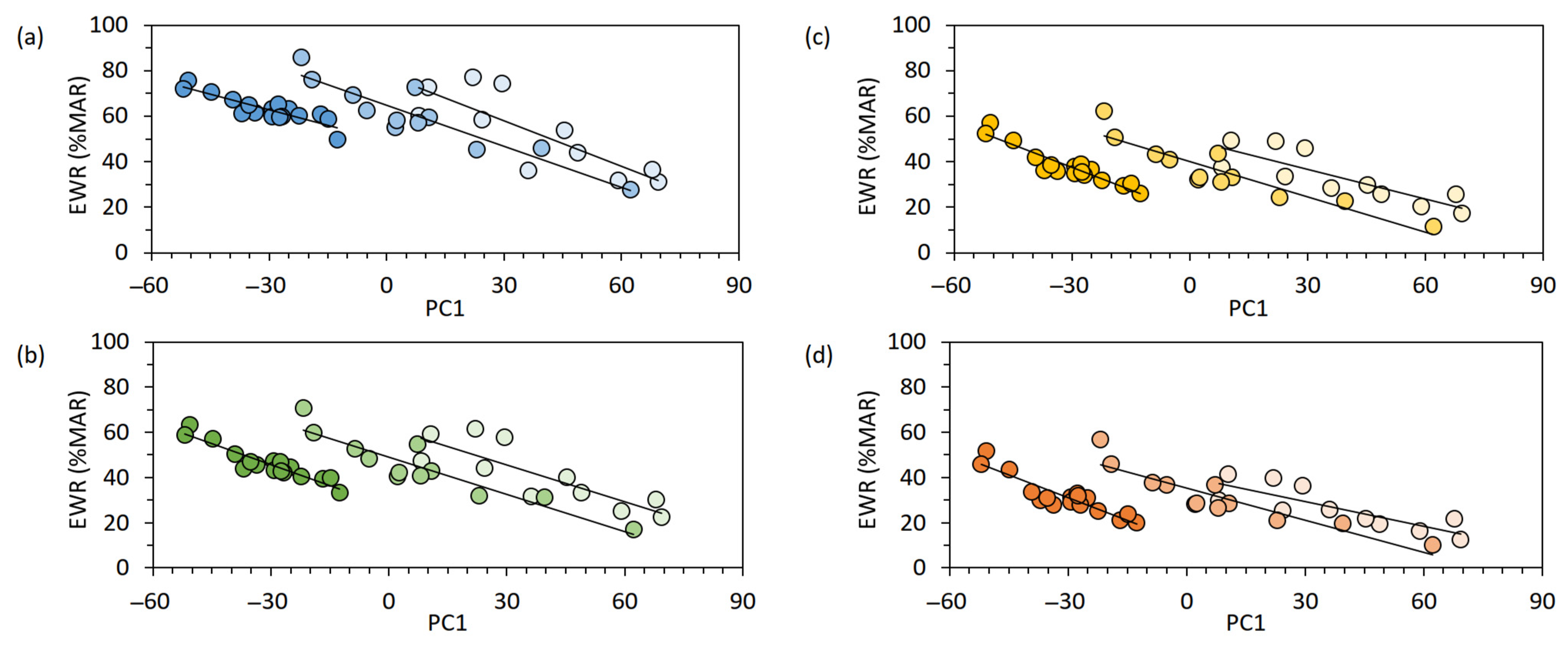
3.2. Environmental Water Reserves’ Reference Values
3.3. Performance of the New Reference Factors for the Frequency of Occurrence
4. Discussion
4.1. Implications and Contributions
4.2. Limitations and Recommendations
5. Conclusions
Supplementary Materials
Author Contributions
Funding
Institutional Review Board Statement
Informed Consent Statement
Data Availability Statement
Acknowledgments
Conflicts of Interest
Appendix A

| Condition | Code | PC1 | PC2 | PC3 | PC4 | PC5 | PC6 | PC7 | PC8 | PC9 | PC10 | PC11 | PC12 |
|---|---|---|---|---|---|---|---|---|---|---|---|---|---|
| Inter-annual | |||||||||||||
| Wet | ACW | 0.98 | −0.16 | 0.03 | 0.02 | 0.05 | 0.02 | 0.00 | 0.00 | 0.01 | 0.00 | 0.00 | 0.00 |
| Average | ACA | −0.93 | 0.28 | 0.21 | −0.08 | −0.02 | −0.04 | −0.01 | −0.04 | 0.02 | −0.01 | 0.00 | 0.01 |
| Dry | ACD | −0.98 | 0.16 | −0.07 | −0.02 | −0.10 | 0.08 | 0.02 | 0.01 | 0.04 | 0.00 | −0.01 | −0.01 |
| Very Dry | ACVD | −0.94 | 0.00 | −0.31 | 0.06 | 0.00 | −0.10 | 0.00 | 0.03 | 0.03 | −0.02 | 0.03 | 0.00 |
| Dry season | |||||||||||||
| Wet | DCW | 0.92 | 0.38 | −0.02 | 0.01 | −0.01 | 0.00 | 0.00 | 0.00 | 0.00 | 0.00 | 0.00 | 0.00 |
| Average | DCA | −0.90 | −0.34 | 0.24 | 0.14 | −0.02 | −0.02 | 0.04 | 0.01 | 0.00 | 0.00 | 0.00 | 0.01 |
| Dry | DCD | −0.91 | −0.39 | −0.04 | −0.02 | 0.00 | 0.05 | −0.07 | 0.01 | 0.00 | 0.00 | 0.00 | 0.01 |
| Very Dry | DCVD | −0.88 | −0.37 | −0.23 | −0.16 | 0.07 | −0.01 | 0.07 | 0.00 | 0.00 | 0.00 | −0.01 | 0.01 |
| Wet season | |||||||||||||
| Wet | WCW | 0.94 | −0.33 | 0.01 | −0.03 | −0.04 | −0.01 | 0.00 | 0.00 | 0.00 | 0.01 | 0.00 | 0.00 |
| Average | WCA | −0.87 | 0.43 | 0.22 | −0.09 | 0.06 | −0.02 | 0.00 | 0.03 | 0.01 | 0.02 | 0.01 | 0.00 |
| Dry | WCD | −0.93 | 0.34 | −0.06 | 0.04 | −0.02 | 0.11 | 0.04 | −0.01 | −0.01 | 0.01 | 0.02 | 0.01 |
| Very Dry | WCVD | −0.92 | 0.14 | −0.30 | 0.18 | 0.05 | −0.06 | −0.02 | −0.03 | 0.01 | 0.04 | −0.01 | 0.00 |
| Statistic | Mann–Kendall Z-Value | P-Value | Sen’s Slope |
|---|---|---|---|
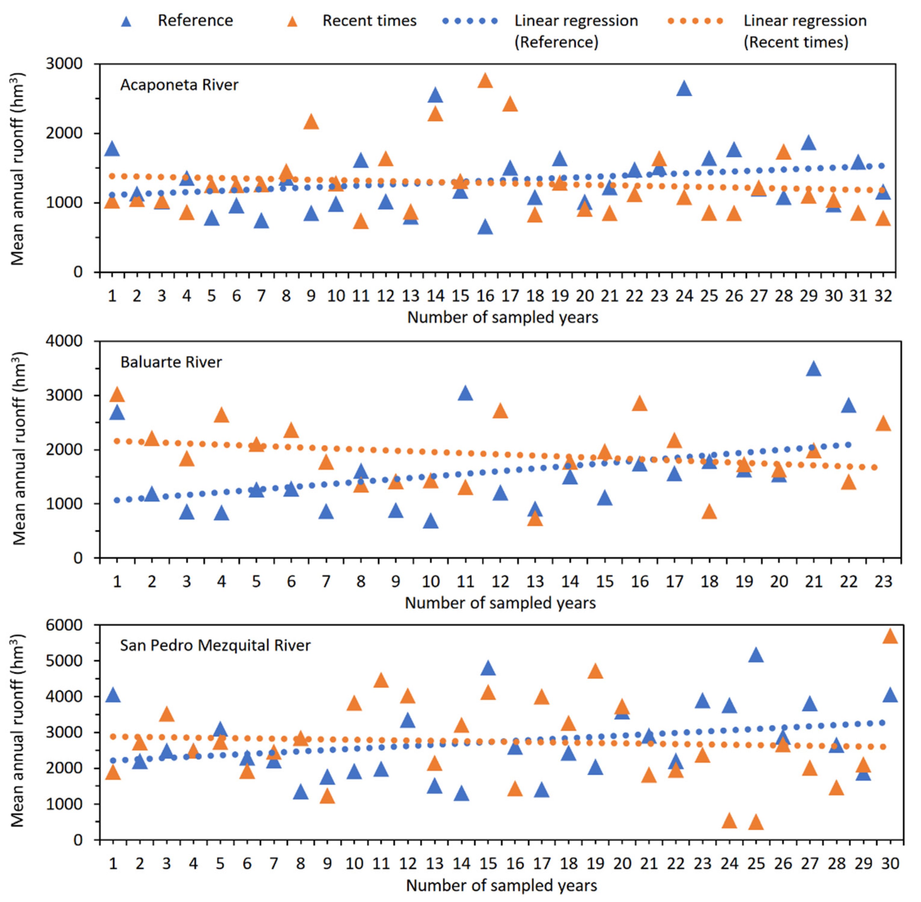
| Acaponeta | |||
| Reference (1945–1976) | 1.8000 | 0.0359 ** | 12.26 |
| Recent times (1977–2008) | −0.7661 | 0.2278 | −5.95 |
| Complete series (1945–2008) | −0.1159 | 0.4539 | −0.34 |
| Baluarte | |||
| Reference (1948–1969) | 2.4814 | 0.0007 *** | 40.28 |
| Recent times (1970–1992) | −1.2149 | 0.1122 | −24.77 |
| Complete series (1948–1992) | 2.2010 | 0.0139 ** | 18.28 |
| San Pedro Mezquital | |||
| Reference (1944–1973) | 1.4630 | 0.0717 * | 33.24 |
| Recent times (1974–2003) | −0.4995 | 0.3087 | −16.21 |
| Complete series (1944–2003) | 0.3125 | 0.3773 | 3.25 |
| Hydrological Condition | Total Sum of Squares | Within-Group Sum of Squares | F | P-Value |
|---|---|---|---|---|
| Tropic of Cancer | ||||
| Wet | 38,460 | 31,190 | 7.694 | 0.0056 |
| Average | 6151 | 5208 | 21.15 | 0.0001 |
| Dry | 4815 | 1760 | 6.89 | 0.0086 |
| Very dry | 3051 | 2667 | 5.47 | 0.0226 |
| Drainage direction | ||||
| Wet | 38,460 | 35,090 | 1.78 | 0.1684 |
| Average | 6151 | 5650 | 1.64 | 0.1867 |
| Dry | 4815 | 4392 | 1.72 | 0.1677 |
| Very dry | 3051 | 2786 | 1.76 | 0.1693 |
| River Type Pairwise | Northern | Southern |
|---|---|---|
| Wet condition of inter-annual, dry, and wet season variability | ||
| Northern | 0.0055 | |
| Southern | 0.0055 | |
| Average condition of inter-annual, dry, and wet season variability | ||
| Northern | 0.00997 | |
| Southern | 0.0097 | |
| Dry condition of inter-annual, dry, and wet season variability | ||
| Northern | 0.0041 | |
| Southern | 0.0041 | |
| Very dry condition of inter-annual, dry, and wet season variability | ||
| Northern | 0.0191 | |
| Southern | 0.0191 | |
| Source | Total Sum of Squares | Degree Freedom | Mean Square | F | P-Value |
|---|---|---|---|---|---|
| Wet | |||||
| Streamflow | 24,940 | 2 | 12,470 | 28.786 | 0.0001 |
| Tropic of Cancer | 6476.3 | 1 | 6476.3 | 14.95 | 0.0001 |
| Interaction | −7682.7 | 2 | −3841.4 | −8.8675 | 0.9998 |
| Residual | 14,729 | 34 | 433.2 | ||
| Total | 38,462 | 39 | |||
| Average | |||||
| Streamflow | 3281.4 | 2 | 1640.7 | 19.917 | 0.0001 |
| Tropic of Cancer | 943.96 | 1 | 943.96 | 11.459 | 0.0004 |
| Interaction | −874.7 | 2 | −437.35 | −5.3091 | 0.3943 |
| Residual | 2800.8 | 34 | 82.377 | ||
| Total | 6151.5 | 39 | |||
| Dry | |||||
| Streamflow | 3055.3 | 2 | 1527.6 | 26.159 | 0.0001 |
| Tropic of Cancer | 855.21 | 1 | 855.21 | 14.645 | 0.0001 |
| Interaction | −1080.9 | 2 | −540.44 | −9.2546 | 1 |
| Residual | 1985.5 | 34 | 58.397 | ||
| Total | 4815.1 | 39 | |||
| Very dry | |||||
| Streamflow | 2204.4 | 2 | 1102.2 | 31.926 | 0.0001 |
| Tropic of Cancer | 383.65 | 1 | 383.65 | 11.112 | 0.0002 |
| Interaction | −711.24 | 2 | −355.62 | −10.301 | 1 |
| Residual | 1173.8 | 34 | 34.525 | ||
| Total | 3050.7 | 39 |
References
- Acreman, M.; Arthington, A.H.; Colloff, M.J.; Couch, C.; Crossman, N.D.; Dyer, F.; Overton, I.; Pollino, C.A.; Stewardson, M.J.; Young, W. Environmental Flows for Natural, Hybrid, and Novel Riverine Ecosystems in a Changing World. Front. Ecol. Environ. 2014, 12, 466–473. [Google Scholar] [CrossRef] [Green Version]
- Acreman, M.C.; Overton, I.; King, J.; Wood, P.J.; Cowx, I.; Dunbar, M.J.; Kendy, E.; Young, W. The Changing Role of Ecohydrological Science in Guiding Environmental Flows. Hydrol. Sci. J. 2014, 59, 433–450. [Google Scholar] [CrossRef]
- Poff, N.L.; Tharme, R.E.; Arthington, A.H. Evolution of Environmental Flows Assessment Science, Principles, and Methodologies. In Water for the Environment: From Policy and Science to Implementation and Management; Horne, A.C., Webb, J.A., Stewardson, M.J., Richter, B., Acreman, M., Eds.; Elsevier: San Diego, CA, USA; Academic Press: San Diego, CA, USA, 2017; pp. 203–236. [Google Scholar] [CrossRef]
- Arthington, A.H.; Bhaduri, A.; Bunn, S.E.; Jackson, S.E.; Tharme, R.E.; Tickner, D.; Young, B.; Acreman, M.; Baker, N.; Capon, S.; et al. The Brisbane Declaration and Global Action Agenda on Environmental Flows (2018). Front. Environ. Sci. 2018, 6, 45. [Google Scholar] [CrossRef] [Green Version]
- Poff, N.L.; Allan, J.D.; Bain, M.B.; Karr, J.R.; Prestegaard, K.L.; Richter, B.D.; Sparks, R.E.; Stromberg, J.C. The Natural Flow Regime. Bioscience 1997, 47, 769–784. [Google Scholar] [CrossRef]
- Richter, B.D.; Baumgartner, J.V.; Wigington, R.; Braun, D.P. How Much Water Does a River Need? Freshw. Biol. 1997, 37, 231–249. [Google Scholar] [CrossRef] [Green Version]
- Hughes, D.A.; Hannart, P. A Desktop Model Used to Provide an Initial Estimate of the Ecological Instream Flow Requirements of Rivers in South Africa. J. Hydrol. 2003, 270, 167–181. [Google Scholar] [CrossRef]
- Mathews, R.; Richter, B.D. Application of the Indicators of Hydrologic Alteration Software in Environmental Flow Setting. JAWRA J. Am. Water Resour. Assoc. 2007, 43, 1400–1413. [Google Scholar] [CrossRef]
- Opperman, J.J.; Kendy, E.; Tharme, R.E.; Warner, A.T.; Barrios, E.; Richter, B.D. A Three-Level Framework for Assessing and Implementing Environmental Flows. Front. Environ. Sci. 2018, 6, 76. [Google Scholar] [CrossRef]
- Tennant, D.L. Instream Flow Regimes for Fish, Wildlife, Recreation and Related Environmental Resources. Fisheries 1976, 1, 6–10. [Google Scholar] [CrossRef]
- Smakhtin, V.U.; Eriyagama, N. Developing a Software Package for Global Desktop Assessment of Environmental Flows. Environ. Model. Softw. 2008, 23, 1396–1406. [Google Scholar] [CrossRef]
- Richter, B.R.; Davis, M.M.; Aspe, C.; Konrad. A Presumptive Standard for Environmental Flow Protection. River Res. Appl. 2012, 28, 1312–1321. [Google Scholar] [CrossRef]
- Organisation for Economic Co-operation and Development (OECD). Water Resources Allocation: Sharing Risks and Opportunities; OECD Studies on Water; OECD Publishing: Paris, France, 2015. [Google Scholar]
- Food and Agriculture Organization of the United Nations (FAO). Incorporating Environmental Flows into “Water Stress” Indicator 6.4.2.—Guidelines for a Minimum Standard Method for Global Reporting; Food and Agriculture Organization of the United Nations (FAO): Rome, Italy, 2019; Available online: https://www.fao.org/3/ca3097en/CA3097EN.pdf (accessed on 5 March 2022).
- Poff, N.L.; Matthews, J.H. Environmental Flows in the Anthropocence: Past, Progress and Future Prospects. Curr. Opin. Environ. Sustain. 2013, 5, 667–675. [Google Scholar] [CrossRef]
- Arthington, A.H.; Kennen, J.G.; Stein, E.D.; Webb, J.A. Recent Advances in Environmental Flows Science and Water Management-Innovation in the Anthropocene. Freshw. Biol. 2018, 63, 1022–1034. [Google Scholar] [CrossRef] [Green Version]
- Capon, S.J.; Leigh, C.; Hadwen, W.L.; George, A.; McMahon, J.M.; Linke, S.; Reis, V.; Gould, L.; Arthington, A.H. Transforming Environmental Water Management to Adapt to a Changing Climate. Front. Environ. Sci. 2018, 6, 80. [Google Scholar] [CrossRef] [Green Version]
- Poff, N.L. Beyond the Natural Flow Regime? Broadening the Hydro-Ecological Foundation to Meet Environmental Flows Challenges in a Non-Stationary World. Freshw. Biol. 2017, 63, 1011–1021. [Google Scholar] [CrossRef]
- Grantham, T.E.; Matthews, J.H.; Bledsoe, B.P. Shifting Currents: Managing Freshwater Systems for Ecological Resilience in a Changing Climate. Water Secur. 2019, 8, 100049. [Google Scholar] [CrossRef]
- Horne, A.C.; Nathan, R.; Poff, N.L.; Bond, N.R.; Webb, J.A.; Wang, J.; John, A. Modeling Flow-Ecology Responses in the Anthropocene: Challenges for Sustainable Riverine Management. Bioscience 2019, 69, 789–799. [Google Scholar] [CrossRef]
- Secretaría de Economía. NMX-AA-159-SCFI-2012 That Establishes the Procedure for Environmental Flow Determination in Hydrological Basins; Diario Oficial de la Federación: Mexico City, Mexico, 2012. (In Spanish) [Google Scholar]
- Salinas-Rodríguez, S.A.; Barba-Macías, E.; Infante Mata, D.; Nava-López, M.Z.; Neri-Flores, I.; Domínguez Varela, R. What do Environmental Flows Mean for Long-term Freshwater Ecosystems’ Protection? Assessment of the Mexican Water Reserves for the Environment Program. Sustainability 2021, 13, 1240. [Google Scholar] [CrossRef]
- Salinas-Rodríguez, S.A.; Barrios-Ordóñez, J.E.; Sánchez-Navarro, R.; Wickel, A.J. Environmental Flows and Water Reserves: Principles, Strategies, and Contributions to Water and Conservation Policies in Mexico. River Res. Appl. 2018, 34, 1057–1084. [Google Scholar] [CrossRef] [Green Version]
- Salinas-Rodríguez, S.A.; Sánchez-Navarro, R.; Barrios-Ordóñez, J.E. Frequency of Occurrence of Flow Regime Components: A Hydrology-Based Approach for Environmental Flow Assessments and Water Allocation for the Environment. Hydrol. Sci. J. 2020, 66, 193–213. [Google Scholar] [CrossRef]
- Méndez González, J.; Návar Cháidez, J.J.; González Ontiveros, V. Analysis of Rainfall Trends (1920–2004) in Mexico. Investig. Geográficas Boletín Del Inst. De Geogr. UNAM 2008, 65, 38–55. [Google Scholar]
- Comisión Nacional del Agua (CONAGUA). Estadísticas del Agua en México; Edición 2018; Secretaría de Medio Ambiente y Recursos Naturales: Mexico City, Mexico, 2018. [Google Scholar]
- Cotler Ávalos, H.; Garrido Pérez, A.; Luna González, N.; Enríquez Guadarrama, C.; Cuevas Fernández, M.L. Las Cuencas Hidrográficas de México: Diagnóstico y Priorización; Pluralia Ediciones e Impresiones: Mexico City, Mexico, 2010. [Google Scholar]
- Martínez-Pacheco, A.H.; Salinas-Rodríguez, S.A. Servidor Cartográfico del Programa Nacional de Reservas de Agua (Versión 10.2); Comisión Nacional del Agua (CONAGUA), Banco Interamericano de Desarrollo (BID) y Alianza del Fondo Mundial para la Naturaleza y Fundación Gonzalo Río Arronte; I.A.P. (WWF-FGRA): Mexico City, Mexico, 2018. [Google Scholar]
- Secretaría de Medio Ambiente y Recursos Naturales. Acuerdo por el que se Actualiza la Disponibilidad Media Anual de las Aguas Nacionales Superficiales de las 757 Cuencas Hidrológicas que Comprenden las 37 Regiones Hidrológicas en que se Encuentra Dividido los Estados Unidos Mexicanos; Diario Oficial de la Federación: Mexico City, Mexico, 2016. [Google Scholar]
- Sonoran Institute Mexico A.C. (SIM). Documento de Evaluación de Caudal Ecológico en las Cuencas Hidrológicas Cerrada Laguna Salada y El Borrego; Programa Nacional de Reservas de Agua. SIM, CONAGUA y Alianza WWF-Fundación Carlos Slim; Sonoran Institute Mexico A.C. (SIM): Mexicali, Mexico, 2015. [Google Scholar]
- Sonoran Institute Mexico A.C. (SIM). Desarrollo de Dos Modelos Precipitación-Escurrimiento para la Estimación de Caudal Ecológico en Dos Sistemas de Cuencas en Baja California Sur. SIM and WWF. Reporte Técnico Final, Convenio PI37; Sonoran Institute Mexico A.C. (SIM): Mexicali, Mexico, 2016. [Google Scholar]
- Instituto Nacional de Estadística y Geografía (INEGI). Conjunto de Datos Vectoriales Escala 1:1,000,0000. Unidades Climáticas. Available online: https://www.inegi.org.mx/temas/climatologia/ (accessed on 5 March 2022).
- Datry, T.; Bonada, N.; Boulton, A. Intermittent Rivers and Ephemeral Streams. Ecology and Management; Academic Press: London, UK, 2017. [Google Scholar]
- Postel, S.; Richter, B. Rivers for Life. Managing Water for People and Nature; Island Press: Washington, DC, USA, 2003. [Google Scholar]
- Richter, B.D.; Warner, A.T.; Meyer, J.L.; Lutz, K. A Collaborative and Adaptive Process for Developing Environmental Flow Recommendations. River Res. Applic. 2006, 22, 297–318. [Google Scholar] [CrossRef]
- Stone, E.; Menendez, L. Natural Disturbance Regime [online]. In Encyclopedia of Earth; Cutler, J., McGinley, M., Cleveland, C.J., Eds.; Encyclopedia of Life, NCSE Online and Media Wiki; Available online: https://editors.eol.org/eoearth/wiki/Natural_disturbance_regime (accessed on 5 March 2022).
- Olden, J.D.; Kennard, M.J.; Pusey, B.J. A Framework for Hydrologic Classification with a Review of Methodologies and Applications in Ecohydrology. Ecohydrology 2012, 5, 503–512. [Google Scholar] [CrossRef] [Green Version]
- Biondi, D.; Freni, G.; Iacobellis, V.; Mascaro, G.; Montanari, A. Validation of Hydrological Models: Conceptual Basis, Methodological Approaches and a Proposal for a Code of Practice. Phys. Chem. Earth. 2012, 42–44, 70–76. [Google Scholar] [CrossRef]
- Warmink, J.J.; Janssen, J.A.E.B.; Booij, M.J.; Krol, M.S. Identification and Classification of Uncertainties in the Application of Environmental Models. Environ. Model. Softw. 2010, 25, 1518–1527. [Google Scholar] [CrossRef]
- Richter, B.D. Re-Thinking Environmental Flows: From Allocations and Reserves to Sustainability Boundaries. River Res. Appl. 2010, 26, 1052–1063. [Google Scholar] [CrossRef]
- Hughes, D.A.; Desai, E.Y.; Birkhead, A.L.; Louw, D. A New Approach to Rapid, Desktop-Level, Environmental Flow Assessments for Rivers in South Africa. Hydrol. Sci. J. 2014, 59, 673–687. [Google Scholar] [CrossRef] [Green Version]
- Poff, N.L.; Brown, C.M.; Grantham, T.E.; Matthews, J.H.; Palmer, M.A.; Spence, C.M.; Wilby, R.L.; Haasnoot, M.; Mendoza, G.F.; Dominique, K.C.; et al. Sustainable Water Management Under Future Uncertainty with Eco-Engineering Decision Scaling. Nat. Clim. Chang. 2016, 6, 25–34. [Google Scholar] [CrossRef] [Green Version]
- Barrios, E.; Escobar, N.; Salinas, S. Cambio Climático, Caudal Ecológico y Seguiridad Hídrica. Análisis de Vulnerabilidad para Siete Cuencas de México; World Wildlife Fund, Alliance for Global Water Adaptation, and Interamerican Development Bank: Mexico City, Mexico, 2019; Available online: https://awsassets.panda.org/downloads/cambio_climatico_caudal_ecologico_y_seguridad_hidrica___wwf_agwa_bid.pdf (accessed on 26 March 2022).
- Mekonnen, M.M.; Hoekstra, A.Y. Four Billion People Facing Severe Water Scarcity. Sci. Adv. 2016, 2, e1500323. [Google Scholar] [CrossRef] [Green Version]
- Tickner, D.; Opperman, J.J.; Abell, R.; Acreman, M.; Arthington, A.H.; Bunn, S.E.; Cooke, S.J.; Dalton, J.; Darwall, W.; Edwards, G.; et al. Bending the Curve of Global Freshwater Biodiversity Loss: An Emergency Recovery Plan. Bioscience 2020, 70, 330–342. [Google Scholar] [CrossRef]
- Krabbenhoft, C.A.; Allen, G.H.; Lin, P.; Godsey, S.E.; Allen, D.C.; Burrows, R.M.; DelVecchia, A.G.; Fritz, K.M.; Shanafield, M.; Burgin, A.J.; et al. Assessing placement bias of the global river gauge network. Nat. Sustain. 2022. [Google Scholar] [CrossRef]
- Boltz, F.; Poff, N.L.; Folke, C.; Kete, N.; Brown, C.M.; St. George Freeman, S.; Matthews, J.H.; Martínez, A.; Rockström, J. Water is a Master Variable: Solving for Resilience in the Modern Era. Water Secur. 2019, 8, 100048. [Google Scholar] [CrossRef]
- Curran, A.; De Bruijn, K.; Domeneghetti, A.; Bianchi, F.; Kyk, M.; Vorogushyn, S.; Castellarin, A. Large-Scale Stochastic Flood Hazard Analysis Applied to the Po River. Nat. Hazards 2020, 104, 2027–2046. [Google Scholar] [CrossRef]
- Sentas, A.; Karamoutsou, L.; Charizopoulos, N.; Psilovikos, T.; Psilovikos, A.; Loukas, A. The Use of Stochastic Models for Short-Term Prediction of Water Parameters of the Thesaurus Dam, River Nestos, Greece. Proceedings 2018, 2, 634. [Google Scholar] [CrossRef] [Green Version]
- Zazo, S.; Molina, J.L.; Ruiz-Ortiz, V.; Vélez-Nicolás, M.; García-López, S. Modeling River Runoff Temporal Behavior through a Hybrid Causal–Hydrological (HCH) Method. Water 2020, 12, 3137. [Google Scholar] [CrossRef]
- Bunn, S.E.; Arthington, A.H. Basic Principles and Ecological Consequences of Altered Flow Regimes for Aquatic Biodiversity. J. Environ. Manag. 2002, 30, 492–507. [Google Scholar] [CrossRef] [Green Version]
- Galeana Herrera, L.; Deputy Director and Technical Secretariat of the National Technical Committee for Normalization of the Environment and Natural Resources, General’s Office for Norms, Secretary of Economy, Mexico City, Mexico; Esteban Marina, A.U.; National Commission for Normalization. Official Communication, 2017.
| Environmental Objective | Frequency of Occurrence of Ordinary or Low Flows Per Hydrological Condition | Frequency of Occurrence of Number of Peak Flow Events | |||||
|---|---|---|---|---|---|---|---|
| Wet | Average | Dry | Very Dry | Cat I | Cat II | Cat III | |
| Ephemeral | |||||||
| A | 0.25 | 0.50 | 0.15 | 0.10 | 10 | 6 | 2 |
| B | 0.15 | 0.45 | 0.20 | 0.20 | 9 | 5 | 2 |
| C | 0.10 | 0.30 | 0.30 | 0.30 | 7 | 4 | 2 |
| D | 0.05 | 0.25 | 0.35 | 0.35 | 6 | 3 | 2 |
| Intermittent | |||||||
| A | 0.20 | 0.45 | 0.25 | 0.20 | 10 | 6 | 2 |
| B | 0.10 | 0.40 | 0.30 | 0.20 | 8 | 4 | 2 |
| C | 0.05 | 0.30 | 0.40 | 0.25 | 6 | 3 | 2 |
| D | 0.05 | 0.20 | 0.40 | 0.35 | 4 | 2 | 2 |
| Perennial | |||||||
| A | 0.10 | 0.40 | 0.30 | 0.20 | 10 | 6 | 2 |
| B | 0.00 | 0.20 | 0.40 | 0.40 | 5 | 3 | 2 |
| C | 0.00 | 0.00 | 0.40 | 0.60 | 3 | 2 | 1 |
| D | 0.00 | 0.00 | 0.00 | 1.00 | 2 | 1 | 1 |
| Descriptor (Index/Metric) | Streamflow Type | |||
|---|---|---|---|---|
| Ephemeral (n = 11) | Intermittent (n = 12) | Perennial (n = 17) | All (N = 40) | |
| PC combination (# basins) | ||||
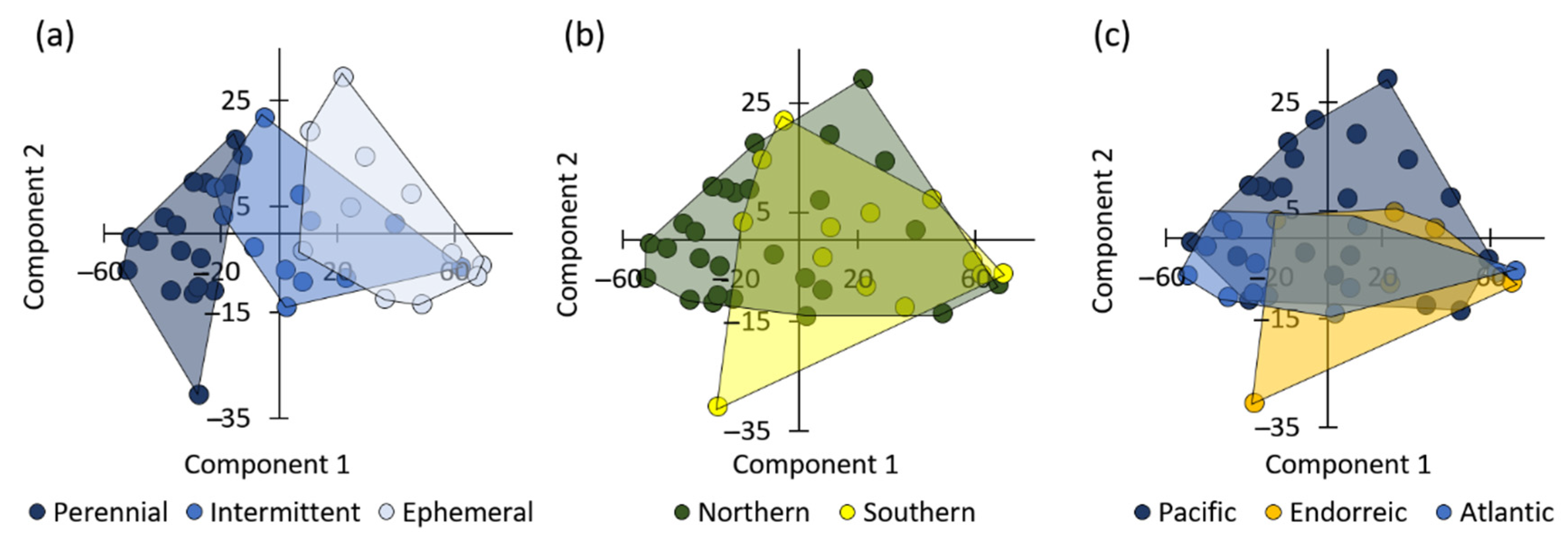
| +PC1 and +PC2 | 5 | 3 | 8 | |
| +PC1 and –PC2 | 6 | 5 | 11 | |
| –PC1 and +PC2 | 3 | 7 | 10 | |
| –PC1 and –PC2 | 1 | 10 | 11 | |
| Coefficient of variation index (CV%) | ||||
| Coefficient of determ. (r2/R2) * | 0.2473 | 0.5071 | 0.4189 | 0.8009 |
| Median | 384 | 228 | 130 | 218 |
| Central range | 339–434 | 207–296 | 111–157 | 134–341 |
| Full range | 271–594 | 154–516 | 64–251 | 64–594 |
| Baseflow index (BFI%) | ||||
| Coefficient of determ. (r2/R2) * | 0.0798 | 0.0008 | 0.1496 | 0.4021 |
| Median | 1.2 | 2.3 | 13.4 | 4 |
| Central range | < 3.9 | 1.2–4.7 | 6.8–25.9 | 1.4–10.0 |
| Full range | < 6.0 | < 7.9 | 1.4–32.5 | 0–32.5 |
| Surface (km2) | ||||
| Median | 2361 | 2891 | 4728 | 3385 |
| Central range | 1425–8748 | 720–8226 | 1849–10,653 | 1354–10,109 |
| Full range | 374–22,927 | 274–17,557 | 483–64,861 | 274–64,861 |
| Dominant climate (%) | ||||
| Semi-warm subhumid | 0.0 | 2.2 | 0.4 | 0.7 |
| Semi-warm humid | 0.0 | 0.0 | 8.2 | 4.6 |
| Warm subhumid | 0.0 | 2.4 | 14.0 | 8.3 |
| Warm humid | 0.0 | 0.0 | 7.8 | 4.4 |
| Semi-dry semi-warm | 5.8 | 9.7 | 5.8 | 6.7 |
| Semi-dry warm | 2.1 | 3.7 | 2.0 | 2.4 |
| Semi-dry temperate | 10.8 | 23.7 | 16.5 | 16.9 |
| Semi-dry semi-cold | 0.0 | 1.5 | 0.1 | 0.4 |
| Dry semi-warm | 25.4 | 15.0 | 2.7 | 10.4 |
| Dry warm | 19.7 | 0.4 | 0.0 | 4.3 |
| Dry temperate | 9.5 | 5.1 | 1.1 | 3.8 |
| Very dry semi-warm | 12.0 | 12.7 | 0.0 | 5.5 |
| Very dry warm | 8.5 | 0.0 | 0.0 | 1.8 |
| Very dry very warm | 0.1 | 0.0 | 0.0 | 0.0 |
| Very dry temperate | 3.1 | 0.0 | 0.0 | 0.7 |
| Temperate subhumid | 1.1 | 18.3 | 33.2 | 22.9 |
| Temperate humid | 0.0 | 0.0 | 1.1 | 0.6 |
| Semi-cold subhumid | 1.9 | 5.4 | 7.0 | 5.5 |
| Hydrological Condition | Total Sum of Squares | Within-Group Sum of Squares | F | P-Value |
|---|---|---|---|---|
| Wet | 38,460 | 13,520 | 34.12 | 0.0001 |
| Average | 6151 | 2870 | 21.15 | 0.0001 |
| Dry | 4815 | 1760 | 32.12 | 0.0001 |
| Very dry | 3051 | 846 | 48.19 | 0.0001 |
| River Type Pairwise | Ephemeral | Intermittent | Perennial |
|---|---|---|---|
| Wet condition of inter-annual, dry, and wet season variability | |||
| Ephemeral | 0.0177 | 0.0003 | |
| Intermittent | 0.0177 | 0.0003 | |
| Perennial | 0.0003 | 0.0003 | |
| Average condition of inter-annual, dry, and wet season variability | |||
| Ephemeral | 0.0141 | 0.0003 | |
| Intermittent | 0.0141 | 0.0003 | |
| Perennial | 0.0003 | 0.0003 | |
| Dry condition of inter-annual, dry, and wet season variability | |||
| Ephemeral | 0.0354 | 0.0003 | |
| Intermittent | 0.0354 | 0.0003 | |
| Perennial | 0.0003 | 0.0003 | |
| Very dry condition of inter-annual, dry, and wet season variability | |||
| Ephemeral | 0.0336 | 0.0003 | |
| Intermittent | 0.0336 | 0.0003 | |
| Perennial | 0.0003 | 0.0003 | |
Publisher’s Note: MDPI stays neutral with regard to jurisdictional claims in published maps and institutional affiliations. |
© 2022 by the authors. Licensee MDPI, Basel, Switzerland. This article is an open access article distributed under the terms and conditions of the Creative Commons Attribution (CC BY) license (https://creativecommons.org/licenses/by/4.0/).
Share and Cite
Salinas-Rodríguez, S.A.; van de Giesen, N.C.; McClain, M.E. Inter-Annual and Seasonal Variability of Flows: Delivering Climate-Smart Environmental Flow Reference Values. Water 2022, 14, 1489. https://doi.org/10.3390/w14091489
Salinas-Rodríguez SA, van de Giesen NC, McClain ME. Inter-Annual and Seasonal Variability of Flows: Delivering Climate-Smart Environmental Flow Reference Values. Water. 2022; 14(9):1489. https://doi.org/10.3390/w14091489
Chicago/Turabian StyleSalinas-Rodríguez, Sergio A., Nick C. van de Giesen, and Michael E. McClain. 2022. "Inter-Annual and Seasonal Variability of Flows: Delivering Climate-Smart Environmental Flow Reference Values" Water 14, no. 9: 1489. https://doi.org/10.3390/w14091489
APA StyleSalinas-Rodríguez, S. A., van de Giesen, N. C., & McClain, M. E. (2022). Inter-Annual and Seasonal Variability of Flows: Delivering Climate-Smart Environmental Flow Reference Values. Water, 14(9), 1489. https://doi.org/10.3390/w14091489