
Reproducing Kernel Hilbert Space Approach to Multiresponse Smoothing Spline Regression Function


Abstract
1. Introduction
2. Materials and Methods
2.1. Multiresponse Nonparametric Regression Model
2.2. Smoothing Spline Estimator
2.3. Reproducing Kernel Hilbert Space
- (i)
- is a vector subspace of (X, ), where (X, ) is a vector space over ;
- (ii)
- is endowed with an inner product , making it into a Hilbert space;
- (iii)
- the linear evaluation functional , defined by , is bounded, for every X.
2.4. Simulation
3. Results and Discussions
3.1. Estimating the Regression Function of the MNR Model Using the RKHS Approach
3.2. Estimating the Symmetric Weight Matrix
3.3. Estimating Optimal Smoothing Parameters
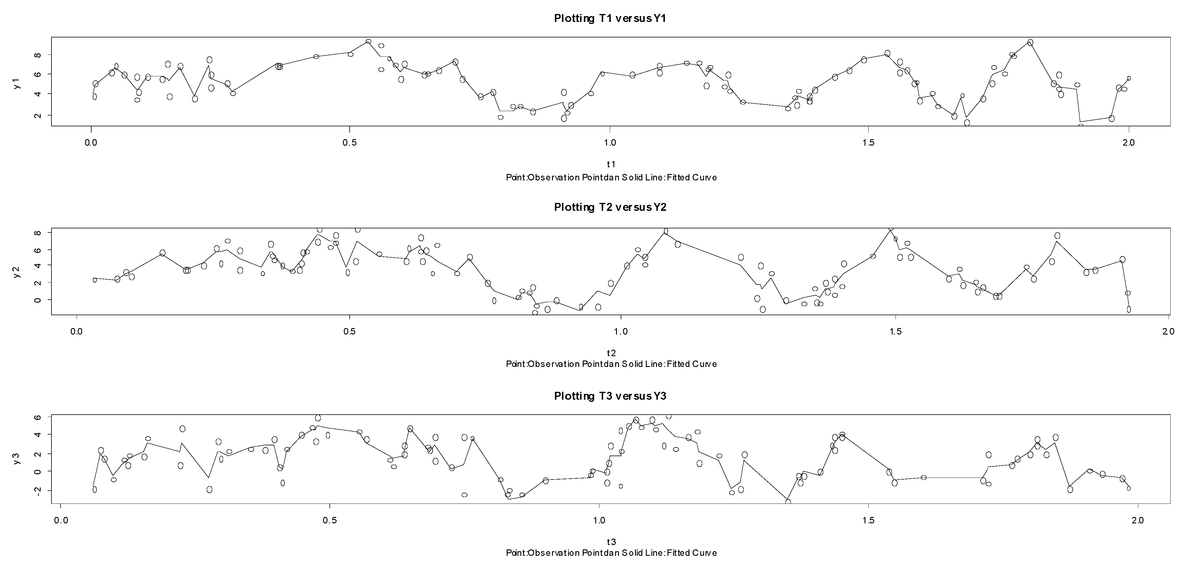
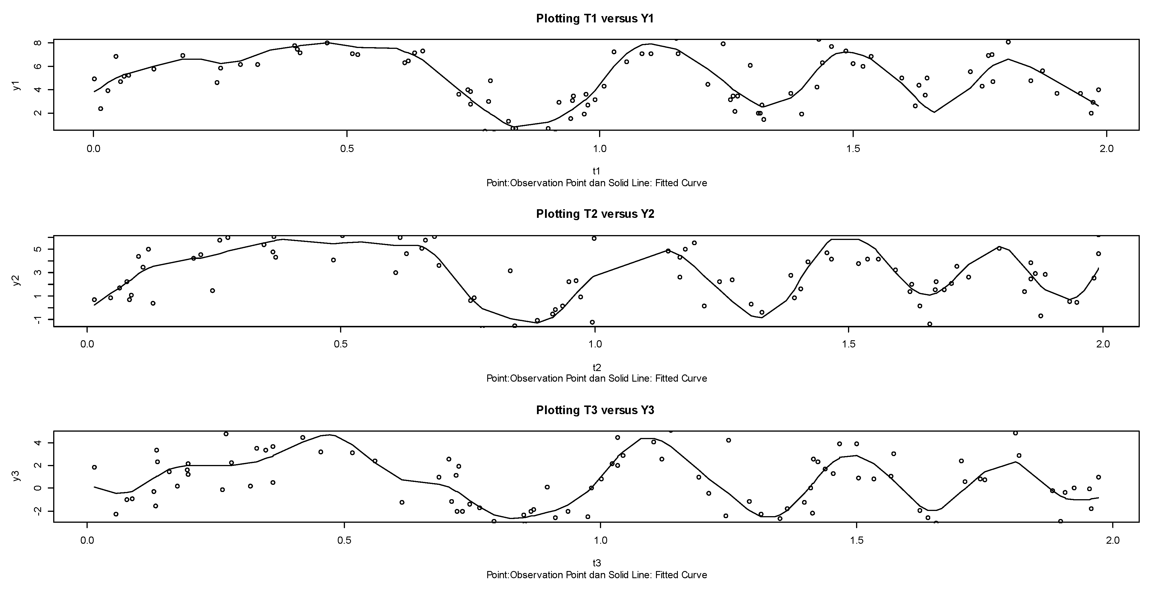
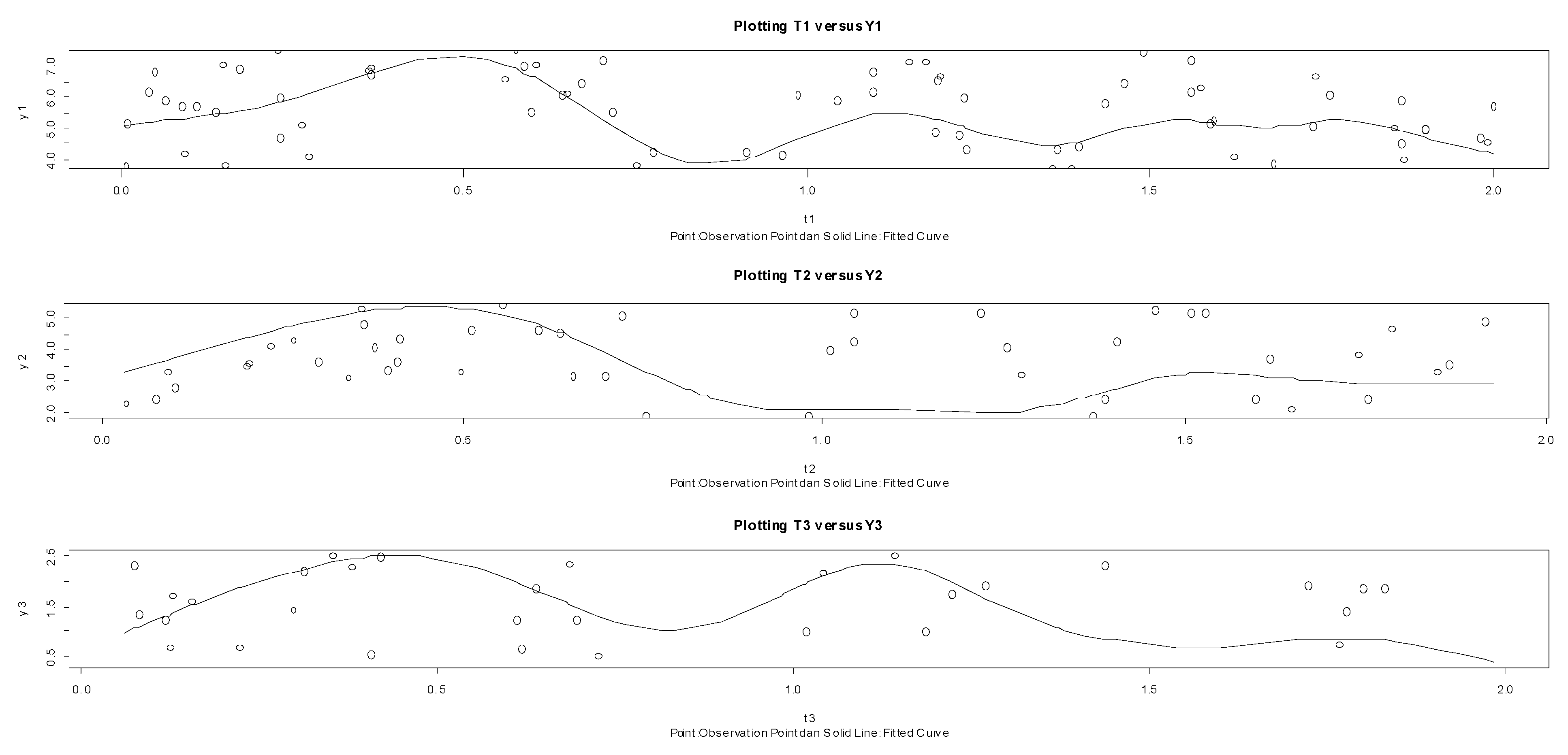
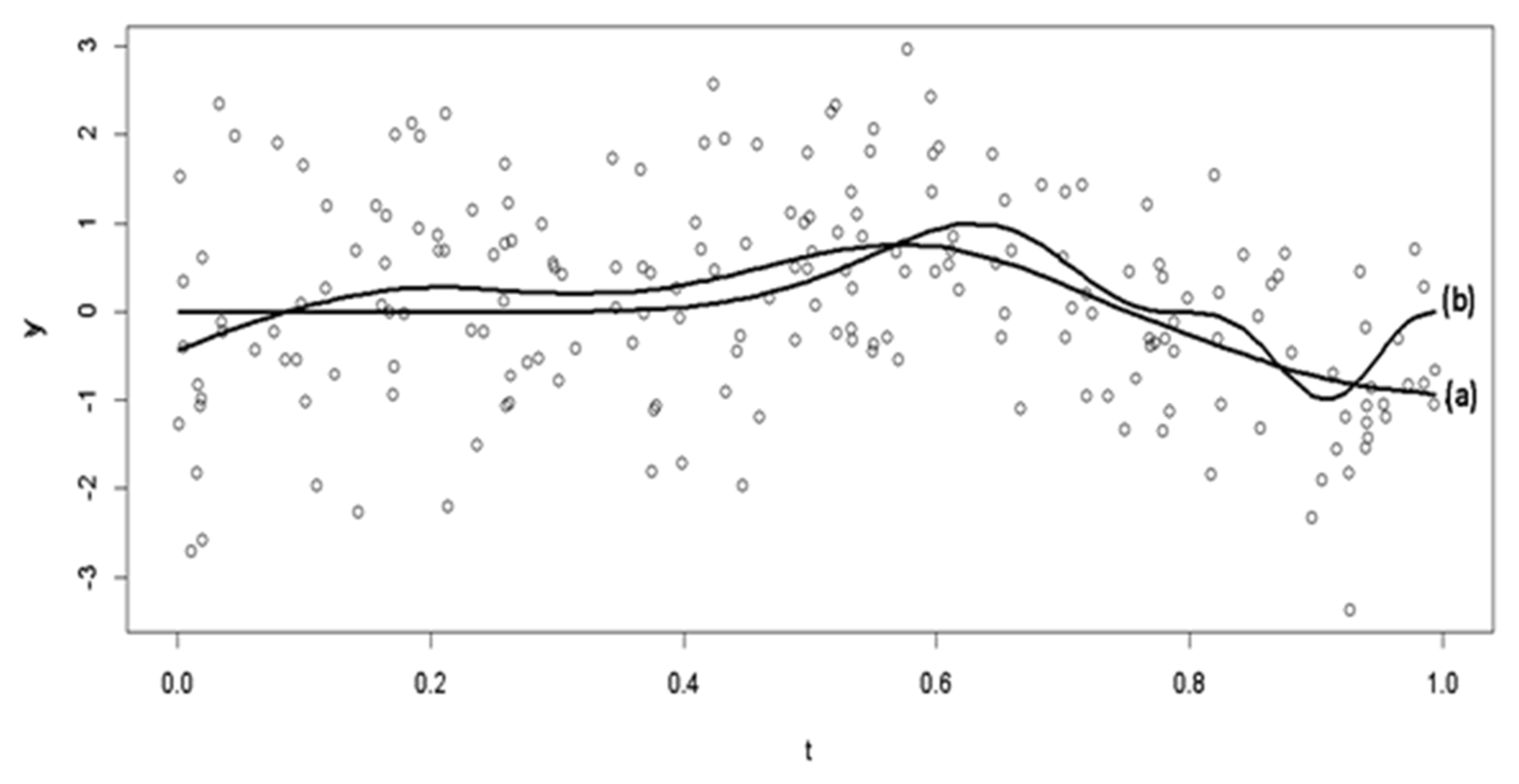
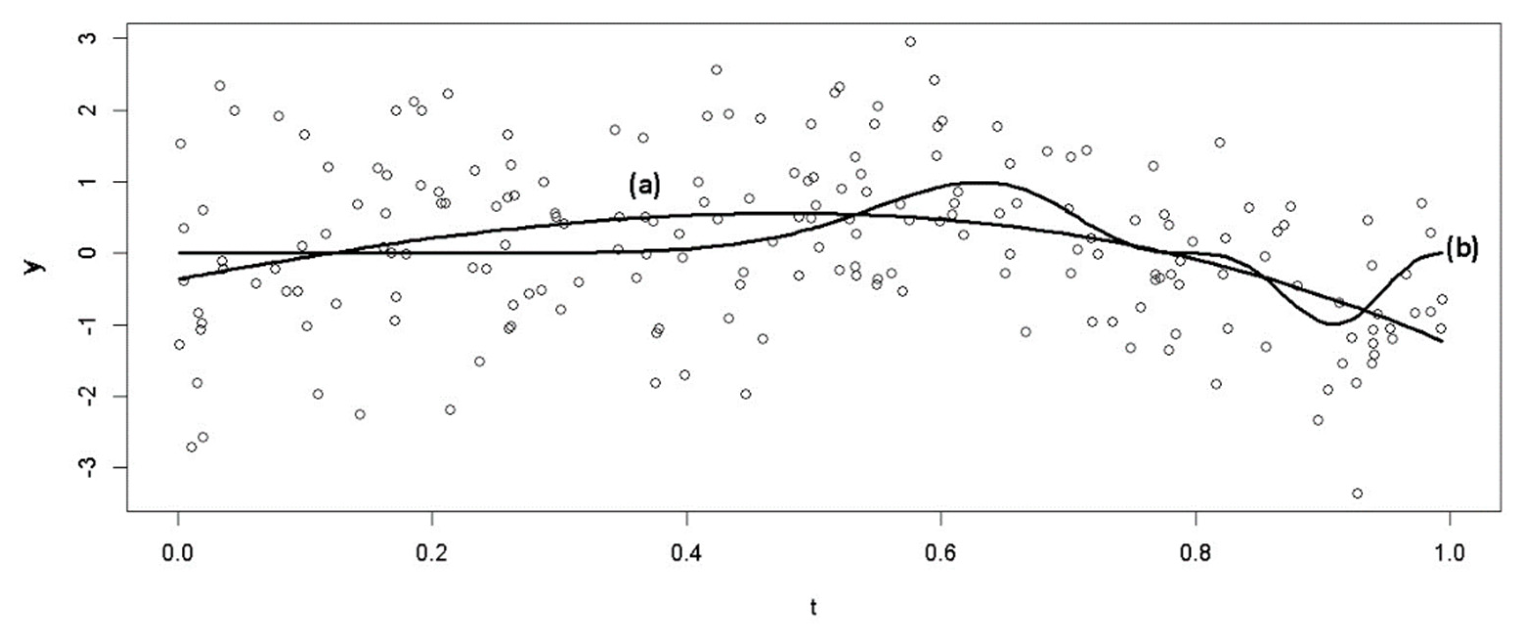
3.4. Simulation Study
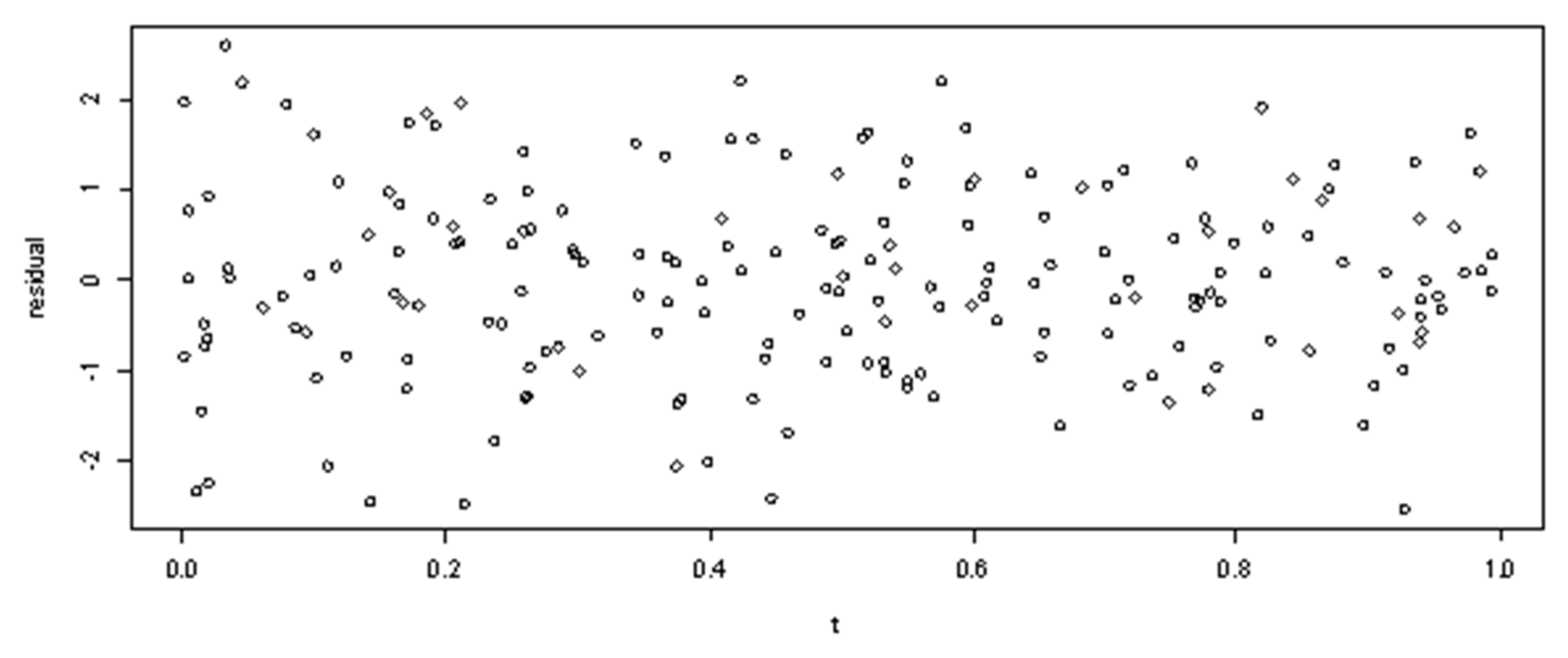
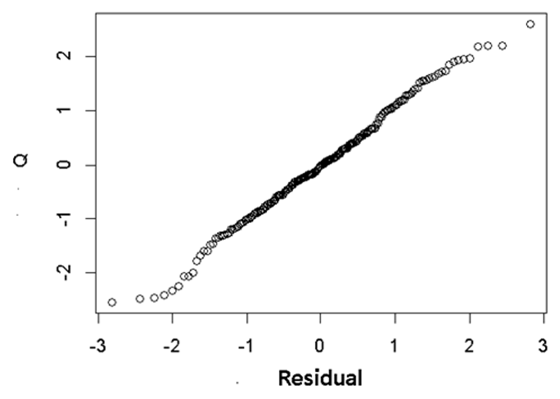
3.5. Investigating the Consistency of the Smoothing Spline Regression Function Estimator
- (A1)
- For every , and .
- (A2)
- For every , .
- (A3)
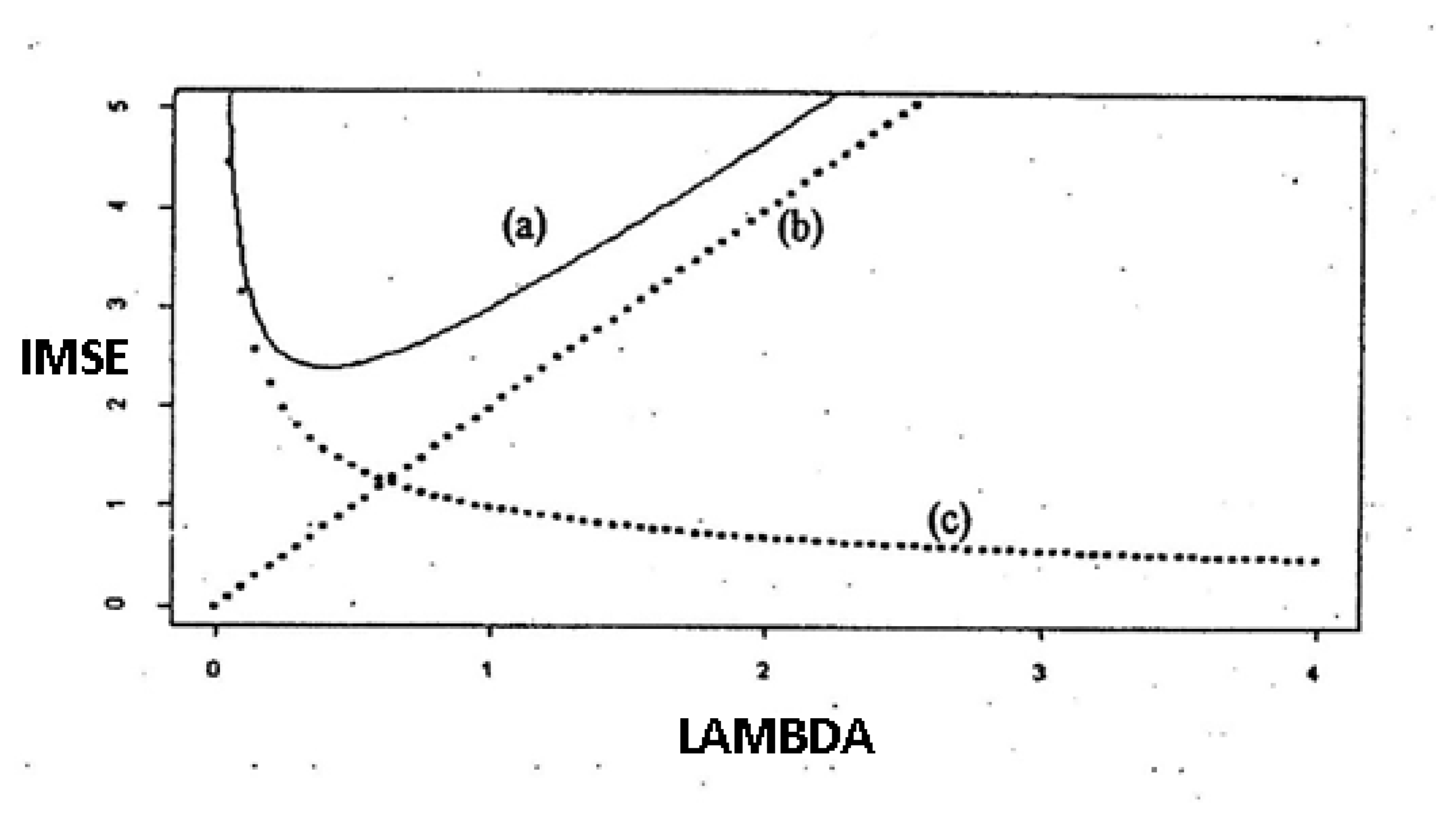
- (a)
- , as .
- (b)
- dt, as .
- (c)
- , as .
3.6. Illustration of Theorems
4. Conclusions
Author Contributions
Funding
Institutional Review Board Statement
Informed Consent Statement
Data Availability Statement
Acknowledgments
Conflicts of Interest
References
- Wahba, G. Spline Models for Observational Data; SIAM: Philadelphia, PA, USA, 1990. [Google Scholar]
- Kimeldorf, G.; Wahba, G. Some results on Tchebycheffian spline functions. J. Math. Anal. Appl. 1971, 33, 82–95. [Google Scholar] [CrossRef]
- Cox, D.D. Asymptotics for M-type smoothing spline. Ann. Stat. 1983, 11, 530–551. [Google Scholar] [CrossRef]
- Oehlert, G.W. Relaxed boundary smoothing spline. Ann. Stat. 1992, 20, 146–160. [Google Scholar] [CrossRef]
- Ana, E.; Chamidah, N.; Andriani, P.; Lestari, B. Modeling of hypertension risk factors using local linear of additive nonparametric logistic regression. J. Phys. Conf. Ser. 2019, 1397, 012067. [Google Scholar] [CrossRef]
- Chamidah, N.; Yonani, Y.S.; Ana, E.; Lestari, B. Identification the number of mycobacterium tuberculosis based on sputum image using local linear estimator. Bullet. Elect. Eng. Inform. 2020, 9, 2109–2116. [Google Scholar] [CrossRef]
- Cheruiyot, L.R. Local linear regression estimator on the boundary correction in nonparametric regression estimation. J. Stat. Theory Appl. 2020, 19, 460–471. [Google Scholar] [CrossRef]
- Cheng, M.-Y.; Huang, T.; Liu, P.; Peng, H. Bias reduction for nonparametric and semiparametric regression models. Stat. Sin. 2018, 28, 2749–2770. [Google Scholar] [CrossRef]
- Chamidah, N.; Zaman, B.; Muniroh, L.; Lestari, B. Designing local standard growth charts of children in East Java province using a local linear estimator. Int. J. Innov. Creat. Chang. 2020, 13, 45–67. [Google Scholar]
- Delaigle, A.; Fan, J.; Carroll, R.J. A design-adaptive local polynomial estimator for the errors-in-variables problem. J. Amer. Stat. Assoc. 2009, 104, 348–359. [Google Scholar] [CrossRef]
- Francisco-Fernandez, M.; Vilar-Fernandez, J.M. Local polynomial regression estimation with correlated errors. Comm. Statist. Theory Methods 2001, 30, 1271–1293. [Google Scholar] [CrossRef]
- Benhenni, K.; Degras, D. Local polynomial estimation of the mean function and its derivatives based on functional data and regular designs. ESAIM Probab. Stat. 2014, 18, 881–899. [Google Scholar] [CrossRef]
- Kikechi, C.B. On local polynomial regression estimators in finite populations. Int. J. Stat. Appl. Math. 2020, 5, 58–63. [Google Scholar]
- Wand, M.P.; Jones, M.C. Kernel Smoothing; Chapman & Hall: London, UK, 1995. [Google Scholar]
- Cui, W.; Wei, M. Strong consistency of kernel regression estimate. Open J. Stats. 2013, 3, 179–182. [Google Scholar] [CrossRef]
- De Brabanter, K.; De Brabanter, J.; Suykens, J.A.K.; De Moor, B. Kernel regression in the presence of correlated errors. J. Mach. Learn. Res. 2011, 12, 1955–1976. [Google Scholar]
- Chamidah, N.; Lestari, B. Estimating of covariance matrix using multi-response local polynomial estimator for designing children growth charts: A theoretically discussion. J. Phy. Conf. Ser. 2019, 1397, 012072. [Google Scholar] [CrossRef]
- Aydin, D.; Güneri, Ö.I.; Fit, A. Choice of bandwidth for nonparametric regression models using kernel smoothing: A simulation study. Int. J. Sci. Basic Appl. Res. 2016, 26, 47–61. [Google Scholar]
- Eubank, R.L. Nonparametric Regression and Spline Smoothing, 2nd ed.; Marcel Dekker: New York, NY, USA, 1999. [Google Scholar]
- Wang, Y. Smoothing Splines: Methods and Applications; Taylor & Francis Group: Boca Raton, FL, USA, 2011. [Google Scholar]
- Liu, A.; Qin, L.; Staudenmayer, J. M-type smoothing spline ANOVA for correlated data. J. Multivar. Anal. 2010, 101, 2282–2296. [Google Scholar] [CrossRef]
- Gao, J.; Shi, P. M-Type smoothing splines in nonparametric and semiparametric regression models. Stat. Sin. 1997, 7, 1155–1169. [Google Scholar]
- Chamidah, N.; Lestari, B.; Massaid, A.; Saifudin, T. Estimating mean arterial pressure affected by stress scores using spline nonparametric regression model approach. Commun. Math. Biol. Neurosci. 2020, 2020, 1–12. [Google Scholar]
- Fatmawati, I.N.; Budiantara, B.L. Comparison of smoothing and truncated spline estimators in estimating blood pressures models. Int. J. Innov. Creat. Change 2019, 5, 1177–1199. [Google Scholar]
- Chamidah, N.; Lestari, B.; Budiantara, I.N.; Saifudin, T.; Rulaningtyas, R.; Aryati, A.; Wardani, P.; Aydin, D. Consistency and asymptotic normality of estimator for parameters in multiresponse multipredictor semiparametric regression model. Symmetry 2022, 14, 336. [Google Scholar] [CrossRef]
- Eilers, P.H.C.; Marx, B.D. Flexible smoothing with B-splines and penalties. Statist. Sci. 1996, 11, 86–121. [Google Scholar] [CrossRef]
- Lu, M.; Liu, Y.; Li, C.-S. Efficient estimation of a linear transformation model for current status data via penalized splines. Stat. Meth. Medic. Res. 2020, 29, 3–14. [Google Scholar] [CrossRef]
- Wang, Y.; Guo, W.; Brown, M.B. Spline smoothing for bivariate data with applications to association between hormones. Stat. Sin. 2000, 10, 377–397. [Google Scholar]
- Yilmaz, E.; Ahmed, S.E.; Aydin, D. A-Spline regression for fitting a nonparametric regression function with censored data. Stats 2020, 3, 11. [Google Scholar] [CrossRef]
- Aydin, D. A comparison of the nonparametric regression models using smoothing spline and kernel regression. World Acad. Sci. Eng. Technol. 2007, 36, 253–257. [Google Scholar]
- Lestari, B.; Budiantara, I.N.; Chamidah, N. Smoothing parameter selection method for multiresponse nonparametric regression model using spline and kernel estimators approaches. J. Phy. Conf. Ser. 2019, 1397, 012064. [Google Scholar] [CrossRef]
- Lestari, B.; Budiantara, I.N.; Chamidah, N. Estimation of regression function in multiresponse nonparametric regression model using smoothing spline and kernel estimators. J. Phy. Conf. Ser. 2018, 1097, 012091. [Google Scholar] [CrossRef]
- Osmani, F.; Hajizadeh, E.; Mansouri, P. Kernel and regression spline smoothing techniques to estimate coefficient in rates model and its application in psoriasis. Med. J. Islam. Repub. Iran 2019, 33, 1–5. [Google Scholar] [CrossRef]
- Lestari, B.; Budiantara, I.N. Spline estimator and its asymptotic properties in multiresponse nonparametric regression model. Songklanakarin J. Sci. Technol. 2020, 42, 533–548. [Google Scholar]
- Mariati, M.P.A.M.; Budiantara, I.N.; Ratnasari, V. The application of mixed smoothing spline and Fourier series model in nonparametric regression. Symmetry 2021, 13, 2094. [Google Scholar] [CrossRef]
- Wang, Y.; Ke, C. Smoothing spline semiparametric nonlinear regression models. J. Comp. Graphical Stats. 2009, 18, 165–183. [Google Scholar] [CrossRef]
- Lestari, B.; Chamidah, N. Estimating regression function of multiresponse semiparametric regression model using smoothing spline. J. Southwest Jiaotong Univ. 2020, 55, 1–9. [Google Scholar]
- Gu, C. Smoothing Spline ANOVA Models; Springer: New York, NY, USA, 2002. [Google Scholar]
- Aronszajn, N. Theory of reproducing kernels. Transact. Amer. Math. Soc. 1950, 68, 337–404. [Google Scholar] [CrossRef]
- Berlinet, A.; Thomas-Agnan, C. Reproducing Kernel Hilbert Spaces in Probability and Statistics; Kluwer Academic: Norwell, MA, USA, 2004. [Google Scholar]
- Wahba, G. Support vector machines, reproducing kernel Hilbert spaces and the randomized GACV. Adv. Kernel Methods-Support Vector Learn. 1999, 6, 69–87. [Google Scholar]
- Scholkopf, B.; Smola, A.J. Learning with Kernels: Support Vector Machines, Regularization, Optimization, and Beyond; MIT Press: Cambridge, MA, USA, 2002. [Google Scholar]
- Zeng, X.; Xia, Y. Asymptotic distribution for regression in a symmetric periodic Gaussian kernel Hilbert space. Stat. Sin. 2019, 29, 1007–1024. [Google Scholar] [CrossRef]
- Hofmann, T.; Scholkopf, B.; Smola, A.J. Kernel methods in machine learning. Ann. Stat. 2008, 36, 1171–1220. [Google Scholar] [CrossRef]
- Johnson, R.A.; Wichern, D.W. Applied Multivariate Statistical Analysis; Prentice Hall: New York, NY, USA, 1982. [Google Scholar]
- Li, J.; Zhang, R. Penalized spline varying-coefficient single-index model. Commun. Stat.-Simul. Comp. 2010, 39, 221–239. [Google Scholar] [CrossRef]
- Ruppert, D.; Carroll, R. Penalized Regression Splines, Working Paper; School of Operation Research and Industrial Engineering, Cornell University: New York, NY, USA, 1997. [Google Scholar]
- Tunç, C.; Tunç, O. On the stability, integrability and boundedness analyses of systems of integro-differential equations with time-delay retardation. RACSAM 2021, 115, 115. [Google Scholar] [CrossRef]
- Aydin, A.; Korkmaz, E. Introduce Gâteaux and Frêchet derivatives in Riesz spaces. Appl. Appl. Math. Int. J. 2020, 15, 16. [Google Scholar]
- Sen, P.K.; Singer, J.M. Large Sample in Statistics: An Introduction with Applications; Chapman & Hall: London, UK, 1993. [Google Scholar]
- Eubank, R.L. Spline Smoothing and Nonparametric Regression; Marcel Dekker, Inc.: New York, NY, USA, 1988. [Google Scholar]
- Speckman, P. Spline smoothing and optimal rate of convergence in nonparametric regression models. Ann. Stat. 1985, 13, 970–983. [Google Scholar] [CrossRef]
- Budiantara, I.N. Estimator Spline dalam Regresi Nonparametrik dan Semiparametrik. Ph.D. Dissertation, Universitas Gadjah Mada, Yogyakarta, Indonesia, 2000. [Google Scholar]
- Serfling, R.J. Approximation Theorems of Mathematical Statistics; John Wiley: New York, NY, USA, 1980. [Google Scholar]


| Smoothing Parameters | Minimum Values of GCV | Results of Estimation |
|---|---|---|
| 4.763234 | The estimation results are too rough. | |
| 2.526286 | The estimation results are the best. | |
| 4.617504 | The estimation results are too smooth. | |
Publisher’s Note: MDPI stays neutral with regard to jurisdictional claims in published maps and institutional affiliations. |
© 2022 by the authors. Licensee MDPI, Basel, Switzerland. This article is an open access article distributed under the terms and conditions of the Creative Commons Attribution (CC BY) license (https://creativecommons.org/licenses/by/4.0/).
Share and Cite
Lestari, B.; Chamidah, N.; Aydin, D.; Yilmaz, E. Reproducing Kernel Hilbert Space Approach to Multiresponse Smoothing Spline Regression Function. Symmetry 2022, 14, 2227. https://doi.org/10.3390/sym14112227
Lestari B, Chamidah N, Aydin D, Yilmaz E. Reproducing Kernel Hilbert Space Approach to Multiresponse Smoothing Spline Regression Function. Symmetry. 2022; 14(11):2227. https://doi.org/10.3390/sym14112227
Chicago/Turabian StyleLestari, Budi, Nur Chamidah, Dursun Aydin, and Ersin Yilmaz. 2022. "Reproducing Kernel Hilbert Space Approach to Multiresponse Smoothing Spline Regression Function" Symmetry 14, no. 11: 2227. https://doi.org/10.3390/sym14112227
APA StyleLestari, B., Chamidah, N., Aydin, D., & Yilmaz, E. (2022). Reproducing Kernel Hilbert Space Approach to Multiresponse Smoothing Spline Regression Function. Symmetry, 14(11), 2227. https://doi.org/10.3390/sym14112227