Review

A Critical Review of Works Pertinent to the Einstein-Bohr Debate and Bell’s Theorem

Center for Advanced Study, University of Illinois, Urbana, IL 61801, USA
Symmetry 2022, 14(1), 163; https://doi.org/10.3390/sym14010163
Submission received: 7 December 2021 / Revised: 30 December 2021 / Accepted: 11 January 2022 / Published: 14 January 2022
(This article belongs to the Special Issue Mathematical Modelling of Physical Systems 2021)

Abstract

:
This review is related to the Einstein-Bohr debate and to Einstein–Podolsky–Rosen’s (EPR) and Bohm’s (EPRB) Gedanken-experiments as well as their realization in actual experiments. I examine a significant number of papers, from my minority point of view and conclude that the well-known theorems of Bell and Clauser, Horne, Shimony and Holt (CHSH) deal with mathematical abstractions that have only a tenuous relation to quantum theory and the actual EPRB experiments. It is also shown that, therefore, Bell-CHSH cannot be used to assess the nature of quantum entanglement, nor can physical features of entanglement be used to prove Bell-CHSH. Their proofs are, among other factors, based on a statistical sampling argument that is invalid for general physical entities and processes and only applicable for finite “populations”; not for elements of physical reality that are linked, for example, to a time-like continuum. Bell-CHSH have, furthermore, neglected the subtleties of the theorem of Vorob’ev that includes their theorems as special cases. Vorob’ev found that certain combinatorial-topological cyclicities of classical random variables form a necessary and sufficient condition for the constraints that are now known as Bell-CHSH inequalities. These constraints, however, must not be linked to the observables of quantum theory nor to the actual EPRB experiments for a variety of reasons, including the existence of continuum-related variables and appropriate considerations of symmetry.
Keywords:
Bell; EPRB; CHSH

1. Introduction

Einstein’s opposition to the probability-related interpretation of quantum mechanics is widely known and attributed by many to an inflexibility of Einstein to accept the new ideas of Bohr’s Copenhagen school [1,2]. Related discussions have all but intensified in recent times and cover several disciplines [3].
The probability interpretation was against Einstein’s intuition, as it may violate the speed of light as a limiting velocity. Naturally, a wave function that permits physical results with finite probability at arbitrary spatial distances cannot obey that limit. The superposition of quantum states, one of the characteristic features of quantum mechanics and interpretations that involve the instantaneous collapse of the wave function upon measurement are clearly difficult to reconcile with the core ideas of relativity.
Einstein had numerous ways to illustrate that situation, including two closed boxes; one containing a marble. Once one box was opened and did not contain the marble, it was known that the other box did. That example evolved into superpositions of exploded and unexploded gunpowder and into Schroedinger’s cat, dead or alive. All of these examples involve quantum entanglement and, in the end, either contradict Einstein’s relativity or represent an incomplete description of physical reality.
Bohr and Heisenberg, on the other hand, went as far as claiming that complementary variables (also named canonical conjugate variables), such as position and momentum, cannot exist as properties of quantum particles but can only be determined in the moment of measurement. Their discussions often went far enough to cast doubts on the physical concepts of space and time altogether.
The height of the discourse was reached in a publication of Einstein, Podolsky and Rosen (EPR) in 1935 [4]. They proposed experiments in which pairs of quantum entities met and interacted and became thus correlated by physical law. Subsequently, the pair was separated and each part sent to a measurement station that was capable of measuring one of two complementary properties of the particles—for example, the position in measurement station 1 and the momentum of the other particle in station 2.
Due to the correlation of the particles by physical law, a situation was considered possible that the position of the particle was measured in station 1 and its momentum inferred from physical law and the measurement in station 2 or vice versa. The claim of Bohr–Heisenberg that position and momentum materialize only in the moment of measurement was thus put in jeopardy.
It took years until an experiment was proposed that indeed could be performed. Bohm suggested that singlet pairs of two quantum entities exhibiting spin, such as photons or neutrons, should be created and then separated and sent toward two distant stations. A spin component (polarization) should then be determined in station 1 and be used to infer the spin component that would be measured in station 2. Such experiments were performed by Kocher and Commins [5] with photons. They confirmed the basic principle proposed by EPRB using parallel polarizers and showed the existence of entanglement over a large distance—large at least on the scale of atomic sizes. The corresponding idealized experiment for photon pairs and Wollaston prisms (which are simply sophisticated polarizers) is discussed in detail below.
In 1964, a new climax was reached on the theory side by a mathematical theorem proposed by J. S. Bell [6] that promised the possibility of a decisive consequence of the Einstein–Podolsky–Rosen–Bohm (EPRB) experiments that followed from measurements with arbitrarily rotated polarizers in the two stations: Bell claimed that the use of Einstein’s “locality condition” (the limiting role of the speed of light) and of “classical” probability theory, make it impossible to obtain all the results that quantum mechanics has provided for EPRB experiments.
This was an unexpected result, because EPRB had eliminated the traps and constraints of the Uncertainty Principle by suggesting to perform only one measurement in each of the two stations and inferring the second not simultaneously measurable complementary property. It was, therefore, expected by Bell, that actual EPRB experiments could, and would, decide the Einstein-Bohr debate.
Clauser, Horne, Shimony and Holt (CHSH) [7] generalized Bell’s theory and, subsequently, extended Kocher’s experiments to rotated polarizers. Aspect [8] and coworkers introduced fast and random switching of the polarizer directions and showed that the CHSH entanglement-correlations were not sensitive to that switching. Zeilinger and coworkers [9] showed these facts over extremely large distances. Of the most modern measurements, the most precise are those of Kwiat [10] as well as Giustina [11] and coworkers, the latter using optical fibers, electro optical modulators as well as extremely efficient solid state detectors (avalanche photodiodes).
All these experiments did indeed show, as postulated by EPR, that measurements in station 2 may be predicted from measurement results in station 1 (and vice versa) with probabilities that approach certainty (more or less). This fact by itself should have ended the Einstein-Bohr discussion. However, this was not to be, because Bell-CHSH did not agree with the totality of the experiments and also not with all the results of quantum mechanics.
As the strictures of the Uncertainty Principle had been removed by EPR and due to a general feeling that classical and quantum probability should not differ too much otherwise as well as because the work of Bell and CHSH appeared to be so elementary that any error was difficult to surmise, there appeared to many only one way out of the discrepancies: to abandon the absolute limitation of “influences” by the speed of light.
It is now widely believed, on the basis of Bell’s work, that entanglement does encompass such instantaneous influences even at large distances. (Note that these influences do not mean instantaneous information transfer, due to the randomness of the possible outcomes of the measurements.)
Greenberger, Horne and Zeilinger (GHZ) [12] even claimed that Einstein’s hypothesis of elements of physical reality can be refuted by a short measurement sequence, and Mermin commented in Physics Today [13] with “What’s wrong with these elements of reality” (see complete story in [1]). It was, however, shown subsequently that the GHZ reasoning amounts to the assumption that, at a certain point of the experiment, a toss of a coin yielding the outcome “head” or “tail” necessitates that the next toss of the same coin will yield the identical outcome. An explicit Einstein local model for the GHZ experiments involving straightforward time dependencies has also been found [14].
The works of Bell and CHSH do not suffer from GHZ’s trivial error (eased by the widespread conviction that quantum entities cannot at all be dealt with by using common sense) but do have a number of issues. Many of these issues have been discussed in a large number of papers, a cross-section of which has been reviewed in recent work by Kupczynski [15]. This latter work contains well over hundred references to important other works of the critical minority–majority discussions that the interested reader may wish to consult. I have included in my review only a very small selection, in order to concentrate on the issues that I find most striking.
I present here a specific concatenation of the issues of Bell-CHSH that are, in my personal view, the most serious. In particular, I concentrate on the fact that quantum and classical probability theories differ by more than the Uncertainty Principle and that the treatments of Bell and CHSH have neglected these other differences in their theory, although these differences could have been included into Bell-type theories and have previously been included in Einstein-type physics. Among these differences are:
  • The probability related work of Bell-CHSH implies that the elements of physical reality are encompassed by a finite number of elements of physical reality, such as Bertelmann’s socks [1]. Relations of the Bell-CHSH elements of reality to continua, such as time-like variables (and corresponding stochastic processes) are incompatible with the Bell-CHSH proofs. Quantum probability for measurements of entangled entities implies no such limitations.
  • Quantum mechanics makes ample use of symmetry laws and merges them with the probability approach by the proper choice of variables; such proper choice of variables may easily be made also for classical probability but Bell and CHSH did not do so.
  • Bell used variations of Einstein’s separation principle that do not have a solid physical basis.
  • Bell and CHSH were not aware of Vorobev’s mathematical theorem [16] that was published two years before Bell’s work and presents the necessary and sufficient condition for the validity of the theorems by Bell and CHSH: the existence of a combinatorial-topological cyclicity of the involved random variables on a probability space. This necessary and sufficient condition has no direct relation to the locality conditions introduced by Bell-CHSH as the basis for their theorems.
It is the purpose of this critical review to show that the above-mentioned neglects of Bell-CHSH have indeed led to the discrepancies between their theory and the experiments as well as quantum mechanics, and that it is not Einsteins separation principle that needs to be abolished. Thus, the results of Bell-CHSH may also not be used to determine the physical nature of entanglement and whether or not entanglement is related to instantaneous influences at a distance.

2. The EPR Gedanken Experiment and Its EPRB Implementation

2.1. Measurements of Spin and Polarization

Figure 1 shows a basic quantum experiment related to spin as described in Feynman’s lectures. Photons are sent from a source S along the z-direction toward a Wollaston Prism that is typically shaped like a cube and is represented in the figure by a square in the x , y - plane that is perpendicular to the z-direction. Through interactions of the photon with the material of the Wollaston symbolized by the shaded circle, the photon is sent either along the black line or the dashed line channel.
These channels are related to the respective H (horizontal) and V (vertical) polarization, as indicated in Figure 1. Such sorting into two channels can be and has been achieved by different types of polarizers, and we use the Wollaston for convenience with the convention that the face of its cube is perpendicular to the z-direction, and the propagation direction of the light (photons). V and H coincide with the x- and y- direction of the face of the Wollaston cube.
For the sake of simplicity of explanation, we assume that the two output channels are also almost parallel to the z-direction (Wollaston cubes close to that property are commercially available). Additional Wollastons subsequent to the first and also oriented in the x , y direction will then conserve the horizontal and vertical channels. It is interesting to note that this possibility of sorting into two channels has been known for about two centuries and, together with Einstein’s photon hypothesis, is completely analogous to the Stern–Gerlach experiments with magnets and spin 1 2 particles. Yet, this latter experiment came as a surprise to the physics world.
Traditional quantum mechanics describes the incoming photons by wave-functions | ψ (spinors) that are transformed by the act of measurement using the Wollaston and assigned a new wave-function denoted either by | H or | V , respectively. No preexisting property of the photons is assumed by traditional Bohr–Copenhagen quantum mechanics. The measurement itself is represented by an operator that, in turn relates to the Wollaston and its geometrical arrangement. Additional subsequent Wollaston prisms will leave the wave function unchanged either | H or | V .
Einstein favored a statistical interpretation of quantum mechanics. According to this interpretation, the photons do have a property, some “marker”, or element of physical reality related to spin or polarization before they are measured. The Wollaston sorts the incoming photons according to this property into two sets S H x and S V y . In the process of sorting, these photons may also be changed and, subsequently, behave precisely like the photons of traditional quantum mechanics when subjected to a sequential suitably oriented Wollaston Prism. The complete set S of all photons emitted from the source is given by S = S H x S V y . We added to the respective sets the subscripts x , y for the following reason:
Any given photon can only be “handled” by one Wollaston Prism with one given orientation. This is where the Uncertainty Principle comes in: The measurement outcome is either horizontal or vertical for the given geometrical position of the Wollaston, which is signified by its coordinates x , y . The horizontal or vertical measurement outcome remains that way if a subsequent parallel Wollaston is used. A rotation of the subsequent Wollaston by some angle a to coordinates x , y sorts the sets S H x ; S V y into new sets S H x ; S V y according to the Malus law involving the relative angle a of the second Wollaston. This sorting is, according to Einstein, due to the elements of physical reality that “mark” the quantum entities and cause the “sorting decisions” by the Wollaston.
In contrast, the Copenhagen school decided against the possibility of such “markers” altogether and rejected Einstein’s statistical interpretation as a possibility; mainly on the basis of the Uncertainty Principle. Einstein at first attempted to unseat the Uncertainty Principle but without success and later changed his strategy and accepted the Uncertainty Principle as an “empirically proven fact”. He came up with an idea for a different method of measurements with the purpose to circumvent the Uncertainty Principle. Bohm’s specialized and perfected version of Einstein’s idea is schematically shown in Figure 2. This version involves correlated photons propagating in opposite directions toward distant Wollaston Prisms.

2.2. EPRB Experiments, Elements of Physical Reality and Entanglement

The schematic experiment shown in Figure 2 uses photon pairs that exhibit, through preparation, certain correlations (entanglement). Such a pair may, in particular, be created as a so-called “singlet” with the property that the measurement outcomes on the two sides are anti-correlated, i.e., horizontal on one side implies vertical on the other and vice versa independent of the chosen Wollaston directions x , y . As discussed, the experiment was designed to decide the question whether quantum particles carry any measurable physical “markers” or elements of physical reality as Einstein suggested. EPR stated [4]:
if, without in any way disturbing a system, we can predict with certainty...the value of a physical quantity, then there exists an element of physical reality corresponding to this physical quantity.
Notice that EPR talked about predicting “the value of a physical quantity”. The equipment may or may not change the physical quantity and assigns it (via the measurement) a value. It is false to believe that Einstein thought that the measurements do not change the quantum entities and determine some absolute property and do not simply “evaluate”. The EPR paper appeared after many discussions with Bohr, Heisenberg and others, and they had agreed on that point. Textbooks and even research papers tend to interpret Einstein in an incorrect way indicating that he did not permit a change of properties by measurement, and then they dismiss his reasoning as prejudicial and classical.
The key idea is that pairs of quantum entities are measured with one entity in each of two distant stations. These pairs of particles are correlated because they are created and interact in a common source and subsequently propagate into different directions. Einstein related these elements of physical reality to mathematical symbols of “hidden variables”, because he suspected an incompleteness of quantum theory, and the EPR and EPRB experiments were designed to investigate these hidden variables.
It is important to realize from the start that one needs two measurements to investigate “hidden variables” because the related elements of physical reality may not yet be recognized. One such measurement needs to put first a value on the hidden variables that may depend also on the measurement equipment. The second measurement is performed on a correlated (entangled) element of physical reality, which is handled by a similar if not identical evaluation equipment (in the present case, a parallel Wollaston). The outcome of this second measurement will then show a relation to the first, because both recognize the correlated (by physical law) elements of physical reality.
There are many examples for classical-macroscopic correlated “particles”, e.g., gyroscopes, that show correlations due to some elements of physical reality. For quantum entities, the correlation is now universally called entanglement and is generally regarded as something entirely different to any classical correlation. It is the main purpose of this paper to present the major reasons of whether both quantum entanglement and correlations of macroscopic entities may be due to elements of physical reality as Einstein suggested.
Of course, entanglement may, in its general physical nature, be very different to standard classical correlations as, for example, those of two gyroscopes propagating in opposite directions. We limit, therefore, all of our discussions of entanglement only to the question of whether or not these correlations may be related to elements of physical reality without involving instantaneous influences over a distance, i.e., we investigate precisely Bell’s question of whether “local hidden variables” are a possibility.
I am fully aware that even this limited view was answered in the negative by Bell and is only considered by a minority, while a large majority has declined the existence of local hidden variables altogether and has accepted, instead, instantaneous influences at a distance.

2.3. Measurements of Entangled Distant Quantum Entities

Experiments corresponding to the scheme of Figure 2 have been performed by several researchers and groups. Kocher, as mentioned above, was the first to show distant quantum entanglement of photons in his thesis with Commins advising [5]. Aspect [8], Zeilinger [9] and related groups have proven the independence of the correlations from the measurement-station distance. Rotational invariance of the correlations, as already found by Kocher, Clauser and others [1], was also confirmed by them.
Anti-correlation of the outcomes can be achieved for 99% of measurement events and maybe even better, as shown by Kwiat [10] and coworkers. Thus, if we measure the outcome H (horizontal) in station 1, then we are virtually certain that the measurement of the photon (belonging to the given pair) in the second station S 2 will result in V (vertcal).
As the events of measurements occur at a large space-like distance, they are separated according to relativity theory, and the correlation must, according to Einstein, arise from some marker, some element of physical reality, that the quantum entities propagating to opposite sides carry with them. Ergo, again according to Einstein, the Copenhagen interpretation is incorrect or at least incomplete, except if one dismisses his claim that the events in the two stations are causally separated and cannot influence each other.
Why, however, should one deny this separation principle of Einstein that has enjoyed, together with the bulk of relativity theory, enormous success in the description of a universe of experiments? Quantum Mechanics and the Copenhagen interpretation have, of course, also shown enormous success, and it is natural that physicists have desired to obtain a decision one way or the other.
Such a decision appeared difficult to impossible until John Stuart Bell [6] proposed an idea that promised to give an experimental distinction between any theory that involved elements of physical reality (some type of markers of the quantum entities) and a theory that did not, such as the quantum mechanics of the Copenhagen school.
Bell and followers discussed the experimental situation of Figure 2 with some addition: the polarizers (corresponding to our Wollaston Prisms) were rotated in time steps between different positions in each station, resulting in measurement pairs for four relative angles between the polarizers. Such angles are frequently referred to as Bell-angles or CHSH-angles. (For the detailed history of contributions see [1]).
Bell claimed in his later work that all these measurements could be explained by quantum mechanics but not by the use of any local theory involving Einstein’s elements of physical reality. In addition, Bell claimed, and this is the current majority view of physicists, that Einstein’s separation principle was, therefore, violated, meaning that there exist instantaneous influences at arbitrary large distances.

3. General Considerations for Modeling EPRB Experiments

The common procedure in work devoted to the Einstein-Bohr–Bell debate is to introduce Bell’s well known paper [6] that presents a classical theory with the additional use of entangled quanta, such as photons. (The term classical theory is often interpreted in different ways, and we, therefore, specify the term further. We refer, with the word “classical”, to an Einstein-type theory for the EPRB that postulates the existence of elements of physical reality and assumes the validity of a classical set-theoretic probability theory [17], of relativity theory and Einstein’s separation principle).
It is then shown that Bell’s classical approach, using such elements of physical reality, leads to contradictions to quantum mechanics as well as experiments. Therefore, it is concluded that such elements do not exist and, consequently, some form of instantaneous influences at a distance must exist. In most cases, that type of discussion leads to a Gordian knot made of strings from the foundations of probability, Einstein’s separation principle, some quantum principles and usually additional assumptions regarding locality that have no direct physical justification (see, e.g. the discussion of outcome independence below).
We proceed here, for reasons of clarity, in a different way and discuss first an example of the separation principle in Einstein’s classical relativity involving two spaceships with identical clocks. We attempt to combine this example with a set-theoretically founded probability theory like that of Kolmogorov in its most basic form. This type of probability theory is a classical way of dealing with probabilities but with a precise axiomatic basis. I do not refer to complicated questions of measure theory that cannot easily be related to physics.
I also discuss, subsequently, a few special properties of quantum probability. These general discussions are directly linked to and compared to EPRB experiments and some important consequences of this comparison are emphasized. Considering these consequences, a precise model a la Bell is presented and compared to the actual model that Bell and CHSH used. The inaccuracies of Bell-CHSH are pointed out, and it is shown that, therefore, neither Bell nor CHSH nor the actual EPRB experiments relate to the nature of entanglement in such a way that one can deduce instantaneous influences at a distance.

3.1. Correlations and Einstein’s Separation Principle in Relativity

Consider two spaceships, one piloted by Alice and the second piloted by Bob; both spaceships carry identically designed clocks. There are a few basic elements in the physical description of the two spaceships with clocks that are relevant to the Bell-CHSH formulation of functions and their theory of EPRB experiments.
  • All the laws for the elements of physical reality within the spaceships are the same and independent of the mostly constant velocities of the spaceships. They are, of course, also the same in the two stations of the EPRB experiments. In addition, physical law connects the two ships and two stations. For example, identical clocks within the two spaceships represent some of these physical laws, and their future readings are correlated in a nonlinear fashion depending on the relative velocities of the spaceships.
    Analogous facts, related to rotational symmetry, hold for the statistical correlations of EPRB experiments.
  • Neither Alice nor Bob can give any prediction about the relative readings of their clocks as long as they have neither theoretical nor experimental knowledge about each other. Bell, CHSH and their followers demand that Alice and Bob still be able to predict the probability for the outcomes of their EPRB measurements in such a way that the outcomes have the precise correlation after merging the data taken in the two stations. This demand represents the core of what is called “the Bell game”.
    The fact that no one can play this game without involving nonlocal effects is taken by many as a proof for the validity of the Bell-CHSH theorems that are seen as consequence of locality assumptions. However, for the case of the two spaceships, the Bell game cannot be played either, as we know from the famous twin paradox. Nevertheless we do not suspect any non-localities or instantaneous influences at a distance in Einstein’s theory of relativity.
    What is overlooked by the Bell-game proponents is the fact that the data of the EPRB experiments are connected in pairs with help of an elaborate space and time system including clocks in the stations that identify and unite the two parts of the entangled pairs. EPRB experiments and their measurement results are not raw data that nature presents but are subject to symmetry laws involving our space–time system, which also determines the relevant physical variables.
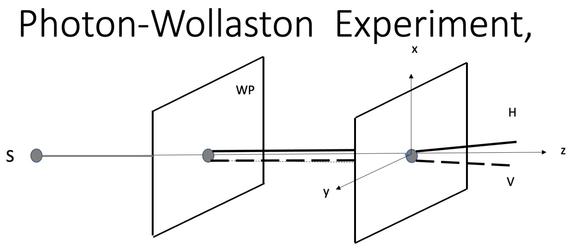
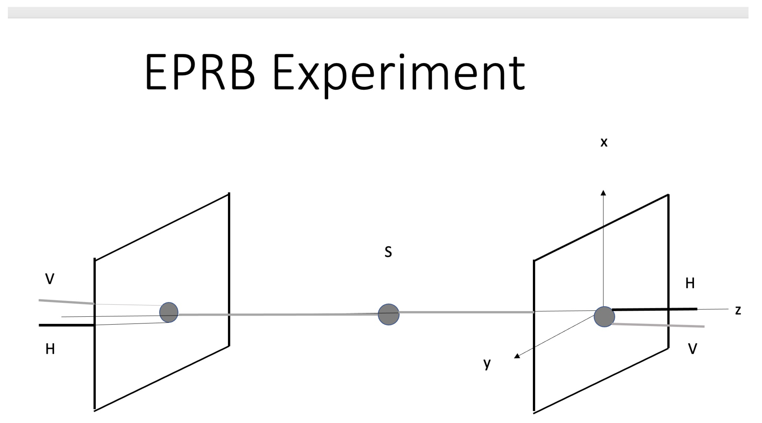
  • In the spaceship example, the velocity of Alice is a “gauge” variable that may be put equal to zero, thus, putting Alice at rest. The clock-reading of Bob depends on the difference of the velocity of his ship relative to Alice’s and does so in a nonlinear way. All of this follows from the invariance to the group of Lorentz transformations. If we assume that the relative clock readings of Alice and Bob depend on some absolute velocity of the spaceships, we would violate the relativistic symmetry.
    The symmetry governing EPRB experiments is the invariance under rotations and the EPRB experiments shown in the above figures are invariant to rotations around the z-axis. As a consequence, the Wollaston coordinates ( x , y -axis) in one given station must also be “gauge” variables that may be arbitrarily chosen. If we rotate the Wollaston of station 2 by an angle θ away from the x-axis, then that θ is the physical variable that describes the change of the statistical correlations as is well known from experiments [5] and quantum theory [18].

3.2. Classical vs. Quantum Probability: Macroscopic Configurations, Symmetries

3.2.1. General Considerations

Classical probability theory includes the concept of time mainly for the case of stochastic processes. Ordinarily, random variables have no time dependence. Tyche, the goddess of fortune, “supplies” some actual element of the sample space Ω of events ω , and as soon as Tyche supplies that actual ω = ω a c t , the random variables that represent physical outcomes of an experiment take on a certain value. One can think of the ω ’s as being simple, indecomposable experiments as described in [17].
For instance, ω can be thought of as being the experiment of sending out a certain correlated pair of quantum entities from a source S to stations S 1 and S 2 . Questions related to reference frames as well as choice of variables and mathematical representations of the data-producing equipment, are assumed to be taken care of by the theorist who creates the probability model.
Tyche is not concerned with symmetry considerations, such as invariance under Lorentz transformations or with configuration-related requirements, such as the spatial extension of dice. Such requirements must be taken care of by the experimenters and theoreticians who choose the random variables (functions on a probability space) that represent the machinery of the actual experiments. Thus, the difficult mathematical and physical choices are not necessarily clearly prescribed by the axiomatic probability framework and the connection of theory and experiments is left to the skills of the theoreticians, which, in certain cases, need to be considerable.
For example, it is entirely possible and an important part of our considerations below that we involve functions on a probability space (random variables), while certain combinations of such functions may lead to contradictions, because the occurrence of different polarizer pairs may lead to demands about the elements of physical reality that cannot be fulfilled.
Quantum mechanics has developed methods that avoid such pitfalls automatically, because it is based on symmetry considerations, plays in Hilbert space and, most importantly avoids the abyss to deal with the outcomes of single measurements, while still producing with expectation values. As a consequence, however, the connection to our accepted space–time system is difficult if not problematic, particularly because the measurement itself is not included in the quantum formalism.
It is mostly the Uncertainty Principle that is blamed for the difficulties. The particular way of EPRB experiments has, however, already circumvented the Uncertainty Principle. Thus, many scientists thought that any additional significant remaining differences mean that our views of physical reality must be revised altogether. However, the classical set-theoretic probability framework does have other significant differences.
For example, if we introduce several equipment configurations during the run of an experiment (as Bell-CHSH do) and if we use the same element of reality in the domain of different Bell-functions, then we introduce the assumption that this same element of reality is indeed available for all these different equipment configurations (such as Wollastons oriented in different directions). Consider, for example, that the elements of physical reality have all different “markers”. Thus, no two of them may be represented by the same mathematical symbol when measured by a Wollaston pointing in different directions at different times.
Quantum probability does not need to concern itself with such questions, but classical probability needs to watch the connection of equipment configurations in space and time and related assumptions about the nature of the quantum entities and the corresponding elements of physical reality. Such assumptions and possible contradictions can usually be taken care of by the use of stochastic processes and the introduction of time-like variables into the probability framework. Bell did not consider this approach.
It also must be noted that quantum probability has, over time, developed very efficient ways to include symmetries of nature, while it takes some doing to include these same symmetries into classical probability theory. The correct physical variables need to be used as the random variables. In the case of spaceships, we need to use the relative velocities as the true physical variable and not any fictitious absolute velocities. Similarly, we need to use the difference between the polarizer angles and not strictly the angles themselves to explain EPRB correlations. This will be discussed in more detail below.

3.2.2. Important Aspects Dealing with Observables and Random Variables

The definitions of the observables of quantum theory and the random variables of classical probability differ in a fundamental way even if one does not deal with non-commutation and the Uncertainty Principle.
I am referring to the following basic facts illustrated for the GHZ experiment [12]. This type of experiment involves four entangled photons that are simultaneously measured either with respect to their linear polarization for which the random variables are denoted by X 1 , X 2 , X 3 , X 4 or for circular polarization with random variables Y 1 , Y 2 , Y 3 , Y 4 . The outcomes of these random variables depend on the polarizer directions or angles, and we denote them by H and V for the horizontal or vertical linear polarization and by L and R for the left circular and right circular polarization, respectively. Thus, we may perform four simultaneous measurements to obtain:
X 1 ( ω n ) = H ; Y 2 ( ω n ) = L ; X 3 ( ω n ) = H ; Y 4 ( ω n ) = L ,
where n stands for the nth measurement of this particular combination. In another measurement, e.g., the ( n + 1 ) ’s, we may obtain:
X 1 ( ω n + 1 ) = H ; Y 2 ( ω n + 1 ) = R ; X 3 ( ω n + 1 ) = V ; Y 4 ( ω n + 1 ) = L ,
It has become customary (but is not always precise enough; see below) to replace the possible outcomes by integer numbers ± 1 , because random variables have usually real numbers for their co-domain and ± 1 reminds us of the possible eigenvalues in quantum theory. Therefore, researchers have chosen + 1 for H and R and 1 for V and L, respectively, which sometimes represents simply a convenient labeling that permits also to use some algebra. For example, the product of the random variables for both above measurements n as well as n + 1 is + 1 .
It represents a grievous mistake, however, to forget about the definition of random variables and continue with the axioms of integers as has unfortunately been done by all researchers supporting the GHZ paper. They assumed, for example that, independent of the number n of the experiment, they may write [12]:
Y i Y i = + 1 ,
with i = 1 , 2 , 3 , 4 being the number of the photon of a simultaneous measurement sequence. However, we have seen from the above equations that we may have
Y 2 ( ω n ) Y 2 ( ω n + 1 ) = 1
Quantum mechanical observables avoid such algebraic inaccuracies, because they involve an operator representing the equipment and a wave function that remind us automatically of possible different outcomes for different measurement sequences.
Therefore, the basic definitions of quantum observables and classical random variables, as well as their relations to actual measurements, quantum preparations and experiments, need to be carefully considered and followed. Using mixtures of the above possibilities and using the algebra of integers instead of the algebra of random variables leads to a comedy of errors, such as published by Greenberger, Horne and Zeilinger [12], approved by Bell [1] and amplified by Mermin in Physics Today [13]. Mermin asked “What is wrong with these elements of reality?” (see also [1]). We know the answer: Mermin’s implementation of the algebra related to random variables is wrong. (For a more detailed explanation see [14].)
The work of Bell-CHSH does not stumble over such elementary problems. As we will see, however, more elaborate problems of similar kind also make it difficult to link Bell-CHSH to actual experiments. More detailed explanations are given in the Appendix A.

4. EPRB Models and Random Variables

4.1. Precise Bell-Type Model with Random Wollaston Orientation

Let us return now to the EPRB experiment of Figure 2 and its actual realization by Aspect and coworkers that includes random and fast switching of the orientation of the Wollaston prisms. This experiment deals with two entangled photons (not with four as the GHZ experiment does).
The information package or quantum entity sent out by the source into two directions is naturally described by a random variable Λ that assumes values of λ n , which represent the elements of physical reality that influence the nth measurement. The orientation of the Wollastons, relative to a given x , y -direction, may be characterized by random variables j and j in the respective stations, which may assume the values given by the angles a , a in S 1 as well as b , b in S 2 .
The measurement outcomes may then be represented by functions A ( j , Λ ) in station S 1 and B ( j , Λ ) in station S 2 , which, by definition, are also random variables. Both the values that Λ and the variables A , B assume need to be dealt with carefully [19]. According to Bell, Λ and the values λ n that it assumes for the nth measurement may symbolize “anything” (that may be called an element of physical reality), which includes measurement times, measurement positions as well as any reasonable physical properties or markers such as necessary to describe phase relations [20]. The variables A , B assume the values H and V.
Let us agree then that we start from any parallel Wollaston configuration (same x-direction, or more generally a configuration of total anti-correlation). The values that A , B assume may then be denoted by H or V, respectively, depending whether the detectors are triggered by channels corresponding to the black line or gray line in Figure 2. Operationally speaking, we also need to note the measurement times t n and t n at which the respective detectors are triggered. We use, for the simplicity of notation below, a common measurement time in both stations.
The possible outcomes for A and B must then be described by symbols, such as ( a , H , t n ) in station 1 and ( b , V , t n ) in station S 2 , respectively. A typical data characterization in station S 1 in terms of functions will then read A ( a , t n ) = H and similar line for station S 2 . The use of time t n in any operational notation has at least four reasons.
  • This reminds us that we are dealing with a different entangled pair (the use of a number n is also sufficient for this purpose).
  • Kocher [21] has shown that the pair emissions from the source exhibit some time dependence. Therefore, for the quantitative description of such experiments the measurement times are needed.
  • We also cannot exclude interactions with the measurement equipment that may depend, for example, on both the Wollaston angle and certain interaction times.
  • The measurement time is needed to identify entangled pairs.
Any deviation from this operational notation imposes conditions on the nature of the elements of physical reality. The inclusion of time-like variables means that it may be necessary to introduce stochastic processes to describe EPRB experiments as has been discussed in several previous publications (e.g., [22,23]).
It is important that the Bell-CHSH model itself must describe pairs of measurement, because it is the entangled pairs that are actually measured. Only for the correlated pairs may we use the elementary events ω n that Tyche provides for the nth measurement and thus obtain:
A ( j ( ω n ) , Λ ( ω n ) ) B ( j ( ω n ) , Λ ( ω n ) ) = A ( a , λ n ) B ( b , λ n ) ,
where the element of physical reality λ n may encompass the actual measurement time t n .
A different pair-experiment must have, in general, a different number n and correspondingly relates to a different ω n as pointed out by the precise probability syntax of Feller [17]. This is important for the Bell-CHSH use of triples and quadruples of pairs. It is also important to keep in mind that the pair expectation values E ( A B ) corresponding to the measured A B products must be functions of j j .

4.2. The Actual Model of Bell-CHSH

The actual model of Bell-CHSH is different from the above precise pair model and considers triples or quadruples that have two different polarizer angles for each of the variables j and j and, correspondingly, four differences j j . These differences are not random as frequently believed but represent the carefully chosen Bell-CHSH angles a b , a b , a b , a b .
Any randomness of the experiments refers exclusively to the order in which these pairs are measured. Subsequently, Bell-CHSH considered large numbers of triple (quadruple) sets of measurement pairs that are obtained by some reordering process after the measurements. That reordering process involves identification of the clicks of an actual pair by synchronized clocks as well as the corresponding angles at these clock-times of actual measurements.
Thus, the concatenated pair-triples (Bell) or pair-quadruples (CHSH) necessitate a description in space and time, which is the basis for the arrangement of the remote components. This is an important point, because it is often said that these triples or quadruples are what nature presents to us locally. The truth is far from that and involves nonlocal knowledge and synchronized clocks and altogether a space–time system and the assumption of equipment-configurations free of contradictions.
There are other major assumptions made in most of the discussions involving Bell-CHSH functions. I have already mentioned that it is commonly assumed that the co-domain of the functions may be described by integer numbers ± 1 that also can be used in algebraic expressions subject to the axioms of integers. The definition of random variables appears to obviate that step. However, it has been pointed out [19] that, while the products in Equation (4) are random variables, complexes of such products, as shown in Equation (7), may not be, at least they may not relate to actual experiments. To use, for example A ( a , λ n ) = + 1 instead of A ( a , λ n ) = V represents a big assumption, because V is related to a certain x , y direction of the Wollaston measurement equipment, and the use of integers looses this connection [20].
Nevertheless, this is what is often the basis for Bell type proofs (see, e.g., Leggetts writings [24] and his statement that the photon “possesses a definite value of the variable A = ± 1 ). Mermin [25], who uses the same simplifications (and additional ones) states:
“Confusion buried deep in the formalism of very general critiques tends to rise to the surface and reveal itself when such critiques are reduced to the language of my very elementary example.”
The inclusion of different numbers n for each different measurement of an entangled pair is already sufficient to derail all the oversimplified Bell-type proofs of Mermin as we will see below, because it removes the Vorob’ev cyclicity that will be discussed immediately. Mermin introduced, in a later publication [26], a sampling theorem that permits a reordering of the λ n s to obtain cyclical quadruples. However, such sampling theorems are only valid for “populations” with finite numbers (countability may be sufficient if the physics permits). As soon as the λ n are chosen for the nth measurement from a continuum, particularly the time continuum, any sampling argument becomes a complicated problem, as is well known from examples of general signal processing (see Appendix A).
It will be shown in the bulk of this review that Mermin’s approach is not “elementary” but oversimplified and does no justice to the complexities of the actual experiments. Similar conclusions have also been reached by other authors (see, e.g., [27]) for a variety of different reasons. With regard to more complex codomains of the Bell functions, see also [28].

5. Vorob’ev and Bell-CHSH-Type Theorems: Constraints for Multiple Pair Measurements

Starting with Boole in 1862, mathematicians have developed a variety of constraints for complexes (e.g., algebraic sums of products of random variables) of three or more random variables and corresponding expectation values. Bell derived such a constraint in terms of his inequality and CHSH generalized his treatment for complexes of four random variables without knowledge of the preceding mathematical work and the corresponding precise necessary and sufficient conditions for the validity of these constraints. They used a variety of premises based on physical considerations that were, as we will see, neither necessary nor sufficient.

5.1. The Theorem of Vorob’ev

The theorem of Vorob’ev [16] is, in this authors opinion, the conclusive work that covers all possible Bell-CHSH type of constraints. It is a very general theorem based on Kolmogorov’s probability theory that involves random variables related to combinatorial-topological cyclicities. The relation to Bell-CHSH was discussed in great detail and more elementary terms in [22].
The Appendix of [20] also presents the Vorob’ev cyclicity in elementary terms, and this review overlaps in several ways with [20], while attempting to present overall a deeper investigation of the crux of the problems with Bell-CHSH. In order to make this review more self-contained and to prime the casual reader with the main points that the Vorob’ev theorem provides us with in relation to EPRB, I am presenting an example that relates directly to the CHSH inequality.
Consider random variables A , A , B , B that may only assume values of ± 1 and are arranged in the following algebraic expression that forms the random Variable Γ :
Γ = | A B + A B + A B A B |
This combination contains a Vorob’ev cyclicity, which is expressed by the fact that the last term on the right hand side of this equation is fully determined once the first three terms are chosen. Note that any random variable that appears identical multiple times in such an expression must represent the same measurement and the same outcome when related to actual experiments.
As one can immediately see by inserting all possible values of ± 1 for the random variables on the right hand side, we have the following constraint for Γ :
Γ = | A B + A B + A B A B | 2
According to Vorob’ev, it is the cyclicity in the expression for Γ that “in the last (sic) analysis is the reason” for any constraints on G a m m a .
If and only if A , A , B , B and Γ are random variables with consistent probabilities and if and only if a cyclicity is formed by the algebraic expression involving A , A , B , B , must we deal with the possibility of constraints. Thus, Vorob’ev’s framework applied to the EPRB situation gives us necessary and sufficient conditions for the existence of the constraints that are imposed by the Bell-CHSH-type inequalities.
Note also that we have now derived a CHSH-type inequality without any word about locality considerations and without any word about elements of physical reality and their mathematical representation by the random variable Λ .
Some of the Bell-CHSH type proofs proceed in that way. We will see, however, that a precise proof that is based on random variables, including Λ , and random variables analogous to Γ and that relates (in a one to one correspondence) to the actual EPRB experiments, is extremely difficult if not impossible to accomplish. As mentioned, if we relate to each product of random variables appearing in the inequality (6) a stochastic process with time-like variables, the proof of Bell-CHSH fails. We will explain this fact further by taking a variety of points of view.

5.2. Theorems of Bell-CHSH and Connection to Vorob’ev’s Cyclicity

The Bell-CHSH constraint is, in its essence, expressed by the following CHSH inequality that has the premise that almost all EPRB data may be described by Bell’s functions and, in turn, may be arranged in quadruples of the form:
| A ( a , Λ ( ω n ) ) B ( b , Λ ( ω n ) ) + A ( a , Λ ( ω n ) ) B ( b , Λ ( ω n ) ) +
A ( a , Λ ( ω n ) ) B ( b , Λ ( ω n ) ) A ( a , Λ ( ω n ) ) B ( b , Λ ( ω n ) ) | 2 ,
It is important to realize that n = 1 , 2 , 3 , . . . , N represents the number of the measurement and does not indicate that the elementary events ω or the elements of physical reality λ are given by a finite number. It is only the number of experiments that is finite. We also see that there is the assumption made that all terms involve the same elementary event ω n that determines the outcome λ n for the random variable Λ .
The cyclicity is expressed by the fact that the last term with the minus sign is fully determined by the previous three terms and the expectation value for the last product can, therefore, not be chosen independently from the other products no matter what probability density of ω is used to start with. A more careful explanation is given in the Appendix of reference [20]. The reader may convince himself by using + 1 and 1 for the possible outcomes. The use of + 1 and 1 and the algebra of integers adds, of course, additional assumptions [20] as already discussed above. Bell’s inequality is a special case of the above CHSH inequality, which is obtained for a = b .
Equation (7) may immediately be turned into expectation values E ( A ( j , Λ ) B ( j , Λ ) ) E ( j , j ) , with j = a , a and j = b , b , and therefore we have:
| E ( a , b ) + E ( a , b ) + E ( a , b ) E ( a , b ) | 2 .
The cyclicity of Vorob’ev is achieved by three factors:
1. The functions A , B are chosen to depend cyclically on the Wollaston angles a , a , b , b . However, these angles are not necessarily the relevant variables of the physics of EPRB experiments (the physical variables are rather the difference between the Wollaston angles as we will see).
2. The ω n are all the same in the measurements with different angle-pairs. This fact needs to be either justified mathematically or physically or both. This is not an obvious fact, because the indices n correspond to different measurements with different entangled pairs and, therefore, to different elementary events ω .
3. The co-domain of the functions A , B has been modeled by the values ± 1 without regard to the actual direction of the Wollastons and the measurement times t n , which may not be a valid procedure (see Equation (5) of [20]).
Thus, Bell and CHSH rediscovered special cases of a general theorem regarding expectation values on probability spaces based on complexes (quadruples and triples) of random variables. On the surface, their premises and derivations appear to use straightforward physics. They did use, however, inaccurate mathematics and oversimplified physics that have been neither necessary nor sufficient to prove their respective theorems as will be shown immediately. Some of these findings have been reported in [29].

5.3. Violations of Probability Syntax by Quadruple Function-Pairs of CHSH

In order to connect the mathematical symbols of any set-theoretic probability theory with the actual measurements and experiments, one needs to link the elementary events ω of the sample space Ω to simple indecomposable experiments [17]. As mentioned, ω can be thought as being the experiment of sending out a correlated pair from S or sending out elements of physical reality (mathematically represented by outcomes λ , of the random variable Λ ). Such a connection to the experiment demands, in general, rules for the definition and logical handling of the elements of physical reality.
For example, on the grounds of basic physics and elementary probability theory, it is impossible to have at any given measurement time period indicated by the EPR clocks and for any given entangled pair two or more different macroscopic configurations or Wollaston angles that are chosen and observed by the experimenter. It is also impossible to send identical entangled pairs simultaneously to more than two different stations with different Wollaston angles.
Quantum mechanics secures such elementary physical demands by playing in a Hilbert space and not being concerned about single outcomes. Classical set theoretic probability theory needs to take care of such facts in different ways. For example, we need to demand that the ω n in inequality (7) may be all different because they belong to different experiments and measurements. If we agree to this natural demand that is commensurate with Feller’s syntax of probability theory, then inequality (7) looses its cyclicity, and all the claims of Bell and CHSH that constraints exist for the Aspect–Zeilinger experiments are null and void.
A more detailed discussion that expresses these facts in a variety of ways can be found in [30]. This reference explains that, while the single pairs in inequality (7) are products of random variables, the complete term with four different setting pairs may not be a legitimate random variable and may not have a well defined expectation value, because it arises from four different experiments.
Many thoughts around this theme have been published by Khrennikov [31] and have been discussed in the many conferences organized by him.

5.4. Are the Wollaston Angles Genuine Physical Variables?

The measurements of relative pair outcomes shown in Figure 2 are invariant to rotations around the z-axis. In other words, we have complete anti-correlation of the outcomes independent of the of actual choice of the x , y -axis of the Wollaston Prisms. As soon as one Wollaston (say Wollaston 2) is turned by an angle θ , that symmetry is broken and a fraction of s i n ( θ ) 2 of the pairs will exhibit equal instead of anti-correlated outcomes.
The interesting fact is that we may obtain the same result, with quantitatively the same fraction of violations of anti -symmetry, if we use an electro optical modulator that “rotates” the polarization of the photons somewhere between the source and station 2 by an angle θ . We conclude from these facts that the angle θ is the genuine physical variable that describes the relative outcomes at the Wollastons, and it is not the absolute Wollaston position, characterized by the x , y -coordinates that determines the relative outcomes.
θ is also the variable quantum theory uses trough introduction of a product Hilbert space. (For the general idea, see [32].) The direction of the x , y -axis is thus only a “redundant gauge” just as the absolute velocity was in the case of the spaceships.
Any educated guess for binary outcomes, involving nonlinear dependencies must involve two probabilities that have a sum equal to 1, such as P 1 = c o s ( F ( θ ) ) 2 and P 2 = s i n ( F ( θ ) ) 2 with:
c o s ( F ( θ ) ) 2 + s i n ( F ( θ ) ) 2 = 1 ,
where F represents, in general, an arbitrary function and plausibly a linear function. This fact was shown with greater rigor in reference [33].

6. Can Bell-CHSH Be Saved?

We can see from the reasoning above that Bell and CHSH use probability theory in such a way that it implies the simultaneous measurability of the same element of physical reality related to photon spin while using different Wollaston directions. This is exactly what the Uncertainty Principle forbids us to do and what Einstein attempted to avoid by proposing to measure exactly one property in each station.
Ways around this problem have been suggested by a number of researchers. We review only a few of these ways all others being combinations of them. What needs to be shown to save Bell-CHSH is that the use of the same ω n in (7) is indeed justified by the mathematical physics of Einstein-type. Here are the ways proposed for justification; all of them incorrect or not applicable to the EPRB experiments and measurements.

6.1. Counterfactual Reasoning

Some reason that one could have measured the same element of physical reality Λ ( ω n ) = λ n for the four different setting pairs, and therefore one would have needed only one pair measurement and should, thus, have obtained the result of all four with one measurement-pair only. No court of justice would have accepted such reasoning, and the actual algebra of Bell-CHSH also has led to an immediate contradiction: after assuming equal λ n in all terms, they obtain by using algebra a term B ( b , λ n ) B ( b , λ n ) for which the λ n actually must be different, because the term symbolizes two measurements with different Wollaston angles in station 2 or alternatively two different angles must have been used at the same time [20]. This points, of course again to the lack of precise treatment of the experimental configurations, which requires the use of stochastic processes to describe the kinematics and dynamics of the situation.

6.2. Reordering of the Elements of Reality

There is an additional and seemingly very plausible way that leads to a Vorob’ev cyclicity of the quadruple-function products that represent possible outcomes. This method is based on the possibility of reordering the λ n such that one obtains all triples or quadruples that exhibit a Vorob’ev cyclicity. A necessary condition for the possibility of reordering is the statistical independence of the λ n from the Wollaston pair settings, which represents one of the reasons for the extensive work on absolutely random switching between these pair settings.
However, this statistical independence is not sufficient to guarantee the possibility of reordering, only necessary. One can convince oneself of this fact by the following counterexample: choose λ from a continuum, for example, related to a time-like variable. The four CHSH pair products relate then to different λ ’s, and the Vorob’ev cyclicity is removed.
Mermin and others used a sampling argument [26], which, in essence, says that each of the different Wollaston pairs samples the same elements of physical reality. They deduced this sampling argument exclusively from the fact that the measurements are performed using fast and random switching between the Wollaston settings, which is at best a necessary condition. What they have not realized are two facts:
First, they need to define the elements of physical reality in their relation to the possible measurements, which means, for the case of random switching, that they need an absolute reference, such as the meter measure in Paris, which does not exist for spin or polarization in stations with different measurement angles. To obtain such a reference free of contradictions, one needs, for example, one Wollaston setting fixed in one station [14,32].
Second, all standard sampling arguments are for finite sets of elements of reality (or depending on the underlying physics perhaps even countable sets). One might think that this is a guaranteed fact for the λ n , because n is limited by a large number N. However, n is only a number labeling the measurement. Yet, λ itself may describe a quantum entity with some wavelike properties that, in turn, may entail phase relations that require a continuum for their description.
Case 1 has been discussed in the subsection about physical variables and also in [20] where it has been shown in the Appendix how the Vorob’ev cyclicity may be removed. One may, of course claim that any definition or “gauge” for the elements of physical reality does not matter as long as we can apply case 2, i.e., Mermin’s “standard” sampling argument, meaning as long as we deal with sets of elements of reality that are comparable to the finite numbers of a “population”.
Assume, for example, that there exist only two elements of physical reality λ 1 = H and λ 2 = V and ignore the fact that H , V have an operational–geometric relation to the Wollaston directions. Such an assumption indeed leads to inequality (7). The proof is simple: one can perform the measurements in sequence for random Wollaston angle pairs and then reorder the measurements such that one obtains the quadruples of (7) with either all V or all H and avoids the problem with simultaneous measurement of impossible configurations.
There is a certain irony in the fact that the Bell-CHSH model leads to contradictions even if we relate λ to two polarization values only. The mere assumption that we deal with four random variables having binary outcomes independent of the Wollaston orientations introduces the Vorob’ev cyclicity. This fact is sufficient to guarantee (7), which, in turn, contradicts quantum mechanics. Quantum mechanics is, of course, not constrained by any Vorob’ev cyclicity, because its observables attribute no significance to the single outcomes. As mentioned, we do not need to restrict ourselves to two values of λ : it is possible to reorder a large number N of the λ n [19].
However, while much of quantum physics deals with a finite number of entities, it also deals with fields. In general, physical models, quantum and classical models, must include continuum considerations related to space–time or continuous “phases”.
In any attempt to admit elements of physical reality, it is certainly necessary to consider such elements related to and having the cardinality of a continuum. The many body interactions of incoming photons with the quantum building blocks of the Wollastons (their constituting atoms, electrons etc.) may point to further elements of physical reality. These may involve, for example, the Wollaston angle a, interaction times Δ t and phase relations ϕ correlated to interactions in the other station.
In other words, functions, like A ( a , λ n , may represent functions, such as A ( a , Δ t , Δ ϕ , . . . ) resulting in a new λ n = ( Δ t , Δ ϕ ) , . . . and similar expressions for other angles and for B in station 2. We clearly deal now with variables that have lost the property of being even countable and, therefore, do not offer the possibility of reordering in any obvious way. Time may certainly enter for a variety of reasons as shown already by Kocher [21] for processes related to the source emission. All of these facts point to the importance of stochastic processes as discussed in many previous publications as necessary to model EPRB experiments [20].
Note that a theory that includes time-dependent processes may also be able to explain why so many experiments, like that of Weihs and coworkers [9], deviate significantly from the straightforward quantum result E ( A , B ) = c o s ( a b ) 2 , with E being the expectation value for angles a , b and outcomes denoted by A , B = ± 1 .
If, however, for additional valid physical reasons, the actual data can indeed be reordered into quadruples that contain a Vorob’ev cyclicity, which implies constraints, then these constraints may not be violated at all no matter whether we talk about quantum or classical experiments and no matter whether or not elements of physical reality exist, as follows immediately from a frequency interpretation of probability.
These considerations certainly show that the experiments organized by Zeilinger and groups using “cosmic randomness” [34] or the free will of coworkers [35] to order the sequence of angle-pairs do not give justification for the Bell-CHSH theory. On the one hand, they cannot guarantee a contradiction-free reference frame [32] for the description of the correlated pairs because of the random switching.
They also cannot justify the reordering and standard sampling arguments if the physical and mathematical description of the pairs involves continua. Such involvement is certainly guaranteed in the classical limit (as shown in the example with circularly polarized wave-packets below). All that these experiments show is a certain unlikeliness of possible interpretations of Bell-CHSH violations related to super-determinism [36].
Mermin’s invocation of sampling arguments, does not work with continuous variables related to the elements of reality, particularly not time-like variables; independent of statistical dependencies. It can be seen from the complications of signal processing and information theory that the continuum case presents no straightforward ways to derive any reordering rules. Vorob’ev simply assumes that his variables are defined on a probability space and identical random variables are related to identical measurement outcomes.
In other words, if a random variable occurs multiply in algebraic expressions, the same outcome needs to be guaranteed for the same ω n ; a guarantee that for multiple EPRB experiments can be provided neither by the syntax of probability theory nor from any known sampling arguments. Bell’s well known proof involving Dr. Bertelmann’s socks (see [1] for the full story) is naturally based on a finite number of socks in addition to other oversimplifications.
Mermin’s error is described in detail in the Appendix, which also explains the differences between reordering requirements to achieve a cyclicity and sampling arguments; all in terms of Mermin’s own mathematical explanations.
Furthermore, the expectation values that are the actual results of the Zeilinger group, depend only on the difference of the Wollaston angles, e.g., a b . This difference is not changed at all by the random process of switching that Zeilinger and coworkers employ. Their statistical results are, therefore, not expected to depend at all on the switching and its randomness, and it makes no difference whether that randomness is derived from star-light or the free will of persons, simply because the Bell-CHSH angles are not randomly changed but kept constant in all of the experiments.

6.3. Listing of Imagined Triples (Another Counterfactual Idea)

A special form of reordering was involved in the inequalities attributed to Wigner and d’Espagnat. It was particularly d’Espagnat [37] who explained that one could write lists of possible outcomes in three Bell-triples instead of in three Bell-pairs, by adding to each Bell-pair an imagined possible outcome C for the third setting:
A ( a , . . . ) , B ( b , . . . ) , C ( ( b , . . . ) ; A ( a , . . . ) , B ( b , . . . ) , C ( ( b , . . . )
A ( b , . . . ) , B ( b , . . . ) , C ( ( a , . . . )
The values of λ n are now irrelevant, and arbitrary long lists of actual results complemented by imagined ones guarantee the existence of joint triple probabilities by the frequency interpretation of probability. This fact suggested to d’Espagnat that the three functions A , B , C are random variables on a probability space and may indeed be used to characterize the actual experiments. Then, a Bell-type inequality follows trivially from line (10). Remembering that Bell-type inequalities are a special case of CHSH for a = b and b = c , we obtain (using A , B , C for the functions with corresponding Wollaston settings a , b , c ) the Bell-type inequality:
| A B + A C + 1 B C | + 2
independent of any elements of physical reality and due to the fact that the above triples can be listed.
The mistake here is that each of the triples of line (10) may have a different joint probability due to the fact that the Cs are arbitrary and imagined (counterfactual again) and the conclusion of d’Espagnat is, therefore, incorrect. A more elaborate description of the inaccuracies of the Wigner-d’Espagnat approach is given in [38].

6.4. Bell’s Factorization and Outcome Independence

The persisting believe in the possibility of saving Bell-CHSH is further based to a large extent on (failed) attempts to factorize Bell’s pair correlation probability density ρ ( A , B | j , j ) as follows [2]:
ρ ( A , B | j , j ) = ρ 1 ( A | j ) ρ 2 ( B | j ) .
This factorization has been justified in a variety of ways, mostly by postulating “outcome independence”. Leggett (see [39] Equation (4)) defines outcome independence by (using our notation):
A ( j , λ n | B ) = A ( j , λ n ) and B ( j , λ n | A ) = B ( j , λ n ) ,
where the symbols | A , | B mean conditional to the outcome of A or B respectively. Such definition is mathematically incorrect. Take, for example, j = j meaning that we have complete anti-correlation. Assume further that A ( j , λ n ) = V . Then, A ( j , λ n | B = V ) represents conditioning to the impossible event, because it violates anti correlation.
If we reformulate this definition in the more usual words “The knowledge that B has occurred does not influence our degree of belief that A has occurred” [17], we must realize that we have used the definition of independent events A and B to start with. Any connection and correlation of the outcomes of A and B by physical law is thus denied. No correlation between the spaceships can exist; not even clocks of the same reference frame may be correlated.
This is, of course, a possible view, if Alice and Bob know absolutely nothing of each other. However, as soon as they bring their data together and involve clock-readings of the timing of the measurements as well as the detection of correlated quantum entities, the possibility of physical laws that correlate the data can no longer be denied. The concept of statistical independence clearly does not follow from Einstein’s separability.
Equation (13) has also been refuted in the literature using a variety of more elaborate reasons (see, e.g., [2]). In addition, basing Equation (13) on locality fails for the spaceship example, because one may not work with absolute velocities. Correspondingly, there are also no absolute angles j = a , b ; j = a , b , because the genuine physical variable for the EPRB correlations is the difference θ = j j as follows from the rotational symmetry. It is difficult to see, how outcome independence can possibly be used as a premise to any general EPRB-related physical theorem.
The factorization has also been shown to be incorrect for many other reasons [40], including the consideration of dynamic effects [41].

7. Bell-Type Models Violating the Quantum Result

The following approaches were designed to rescue Bell’s theorem by showing that certain Bell-type models could not obtain the quantum result.

7.1. Larsson’s Pie Chart

Larsson [18] presented a linear pie chart model that easily explains the complete anti-correlation results. It is well known and frequently used to illustrate that the quantum mechanical result for photons P ( j , j ) = P ( j j = θ ) = c o s ( 2 θ ) may only be approximated by the straight line P ( θ ) = 4 π θ 1 , with 0 θ π 2 when using the Bell-CHSH theory. Larsson had not seen the theorem of Vorob’ev at this time of introducing his pie chart and did not realize that the existence of a cyclicity depends on the way that P ( θ ) is measured.
If, for example, the angle j is fixed to j = a and only j is varied to obtain a value of 0 θ π 2 , then no Vorob’ev cyclicity exists as is easily checked out and shown in great detail in the Appendix of [20]. The measurements of Kwiat (see Kwiat and coworkers [10] and their Figure 2a) are performed that way and still represent the most precise EPRB data in excellent agreement with quantum mechanics.
Larsson’s pie chart approximation and the claim of necessity of linearity because of the Bell-CHSH work, has led many researchers to the circular logic that the Bell’s inequalities may not be violated. A simple Einstein local counterexample with fixed setting in one station and in complete agreement with the measurements of Kwiat and coworkers [10] has already been published in 2006 [29].

7.2. The Malus Law and EPRB

A favorite way to show that the quantum laws cannot be derived by the approach of Bell, is by way of counterexample based on a twofold application of the Malus law. It is pointed out that the quantum mechanical description of the singlet pair at the source relies on a superposition of states. This superposition, involving Hilbert space, is then put in juxtaposition to the following postulate.
Bell’s λ n , the elements of physical reality leaving the source, cannot be related to the Wollaston angles, which may be rapidly and randomly changed. Nevertheless, some definite “model-value” is attributed to them that relates somehow to a fixed linear, circular or elliptic polarization. Such an attribute is implied in the work of Larsson [18] and explicitly described by Leggett [39].

7.2.1. Problems with the Double Malus Model

Reasoning of this kind naturally leads to applying the Malus law twice, once on each side by using the given polarization that is ascribed to the photon at the source. Its measurement outcome is then derived from the Malus law by using the angle with respect to the angle of the Wollaston at the time of measurement: α j for one station and α j for the other. (The complications of circular and elliptic polarization are discussed in the example below).
One thus applies the Malus law twice, exactly as one would do if one had a given polarization corresponding to Bell’s λ n . Any relation of λ n to a definite polarization is, however, problematic for the following reason. The measurement-outcome-value is determined by both the properties of the entangled pair and the respective equipment settings. It is, therefore, logically problematic to assign to λ n some value related to “horizontal” or “vertical” if the polarizers in the two wings are not parallel.
The procedure would only be precise, if indeed an entity would be emitted, say into the right wing of the experiment and measured by a first polarizer that defines what “horizontal” or “vertical” really means (consistent with what it means at the moment of measurement) and the so-prepared entity is then subsequently measured by a second polarizer, which is rotated by some angle α j relative to the first (and a similar procedure with α j in the other wing). For the actual EPR experiment, however, a consistent value of “horizontal” or “vertical” that is now firmly related to λ n can only be assigned for parallel polarizers in the two wings. For not parallel polarizers, the Malus law cannot consistently be applied twice, because “horizontal” and “vertical” means something different in the two stations.

7.2.2. Single Malus Model

The way one needs to explain the actual EPRB experiments is the following. The first Wollaston in station 1 measures an entity of which a correlated counterpart has been sent to station 2. As soon as one measures in station 1 and obtains a result of say “horizontal” one is also sure that one will measure “vertical” in station 2 if j = j . If, however, j j and j j = θ , one still may guess the probability with the Malus law but now only for a given outcome in one station.
For example, if we have a “horizontal” outcome in station 1, we have the probability c o s 2 ( θ ) for a “vertical” outcome in the station 2. Thus, one uses the Malus law only once after a measurement has been performed, and indeed one obtains the quantum result (this was discussed by Jung [42] in some detail using wave arguments, i.e., reasoning that applies only for the classical limit). In this way, Alice can predict the probability of Bob’s outcome after she has made her measurement and vice versa.
It is quite usual for quantum problems that the probability for certain outcomes to occur depends on factors that may only be determined by a test measurement or preparation, which, in turn, may change the quantum entity. For our particular EPRB experiment, this change does not matter, because we are dealing with distant correlations and not immediate causal consequences.

8. Why Bell-CHSH Cannot Be Saved: An Explicit Einstein-Local Counterexample

We now present an Einstein type model, with local elements of physical reality, for the experiments of Aspect, Zeilinger and related groups. We use the mathematics of circular polarized light packets or circularly polarized photons. An attempt of this kind was made by Leggett [39] who used the Malus law twice as described above and, therefore, could not come up with a local model. Another attempt was presented by Jung [42] who used the Malus law correctly and successfully but stayed within the confines of a wave-picture.
Quantum mechanically speaking, a right-hand circular polarized photon may be described by a state | R and a left hand circular polarized photon by | L (see Feynman [43] p. 11). There appears to be the puzzle, related to both the classical field formalism and the quantum formalism, that the polarized entities do not appear to have any relations to the coordinates of the Wollastons.
Feynman [43] had already noticed this puzzle and solved it for the quantum formalism. Feynman states: One may use the circular polarized states | R and | L as quantum basis states and can forget then about the x , y -axes. “Isn’t that nice-it doesn’t take any axes..... On the other hand isn’t it rather a miracle that when you add left and right together you can find out which direction x was”. Feynman then derives two states | R , | L for coordinates x and y that are obtained rotating the Wollaston by an angle θ and finds
| R = e ( i θ ) | R and | L = e ( + i θ ) | L ,
from which Feynman concluded that the phase relation of the right and left circular polarized states keeps track of the x direction.
From the viewpoint of the hypothesis involving elements of physical reality and from the fact that the EPRB correlations are a function of θ , one must conclude the existence of some additional “marker” that is the origin of the nonlinear statistical dependence on θ .
To illustrate these facts, I present a model that has been derived previously in slightly different form [29]. (Regarding a version using a classical wave picture see also [42] and [44].) Included into this model is a set of hidden variables λ n R and λ n L representing elements of physical reality corresponding to circular polarizations R or L, respectively, in the two stations of the EPRB experiments.
We describe only the case of right circular polarization R toward station 1 and L toward station 2. We assume that any consequences of possible space–time dependences are absorbed into both λ n R and λ n L , which thus need to be chosen from a continuum and we choose them from the unit interval [0, 1] of the real numbers. The angle j of the Wollaston in station 1 may be set to a = 0 , because it represents, as explained above, a gauge variable.
The angle of the Wollaston in station 2 is at first also chosen to be 0, in order to establish complete anti-correlation, and then rotated to θ . As discussed above, the actual measurements and experimental settings as well as the collection and ordering of the data in pairs involve extensive use of our space–time system as well as clocks. We then denote our Bell-functions by A ( 0 , λ n R ) and B ( θ , λ n L ) and choose the following convention for the possible measurement outcomes:
A ( 0 , λ n R ) = H
for all λ n R and
B ( θ , λ n L ) = V
if and only if
λ n L 1 2 ( 1 + c o s ( 2 θ ) )
Using the frequency interpretation of probability, we find that the probability P θ for B resulting in V (for vertical) is given by:
P θ = ( c o s θ ) 2 .
We proceed analogously for the case when left circular polarized photons propagate to station 1, with the outcome V in station 1 and H in station 2, respectively. The resulting possible outcomes agree with quantum mechanics.
Followers of Bell-CHSH may protest that the use of θ represents a nonlocality. However, as we have seen, the space–time system is used in an elaborate way to pair the data, and we are facing here the usual fact that science exorcises the spooky influences at a distance by introducing the power of the space–time system. In addition, if this protest had any “teeth”, then the Bell theorem would be proven by the mere fact that the pair expectation values depend on θ , and there would be no need to consider triples as Bell did or quadruples as CHSH did.
There are some subtleties in the above approach: Alice and Bob cannot predict the actual outcome for A , B that they will record next if they are not informed about the conventions of Equations (15)–(17) that include global gauge for right and left circular polarization. Only if Alice knows that her outcome is H and that θ = 0 , can she predict that Bob’s outcome will be V. It is nonsense to ask Alice and Bob (or any theoretician) to somehow deduce the global correlations without them both knowing θ . In addition, the λ n R or λ n L are chosen from a continuum, as perhaps related to a relative phase or some relative occurrences in space–time. This fact by itself invalidates the sampling argument by Mermin and others.
The failures of previous models, particularly the one introduced by Larsson [18] arise from the attempt to work with linear functions and to apply the Malus law twice from the source toward station 1 and 2, respectively, while, at the source, there cannot be any information toward which measurement angles the Wollastons actually will be rotated in the moment of measurement. Thus, the rotations of the angles that are performed to assure Einstein separation and the reordering hypothesis, actually prevent the development of valid double-Malus models.
Is the above example still subject to any CHSH constraint at all, for reasons not yet discussed? Any other constraint is unlikely, because the real variables in any pair-experiment are not the Bell-CHSH angles but only their differences. A Vorob’ev cyclicity and, therefore, a constraint may only be achieved by special experimental circumstances. If, however, the data pairs can indeed be reordered into CHSH quadruples, then not even quantum mechanics can contradict these measurement outcomes and the CHSH theorem.

8.1. Closing Loopholes

The above considerations demonstrate that the theorems of Bell-CHSH are special cases of a mathematical theorem that has been treated in the literature since Boole’s work of 1862 and perfected by Vorob’ev in 1962, who gave necessary and sufficient conditions for all related theorems. The conditions used by Bell-CHSH and followers, particularly the outcome independence suggested by Bell, Leggett and others (as explained above) as well as Mermin’s sampling argument are not applicable to EPR and EPRB experiments as soon as continua (related to phases, fields, space–time etc.) are admitted to influence the elements of physical reality and their physical properties. These facts have not been acknowledged by the supporters and followers of Bell for reasons unknown to this author.
Bell was, of course, aware that the contradiction of his theorem and quantum mechanics, if indeed defensible, had major consequences for the interpretation of entanglement over a space-like distance. He was convinced that “locality" was at least a necessary condition for his theorem and he saw immediately that instantaneous influences over a distance could lead to violations of his theorem. From these facts, he deduced that, in order to show the revolutionary character of his findings, one only had to rule out any communication between the stations that were limited by the speed of light.
The first important experimental contributions by Kocher and Commins as well as others (see the detailed story in [1]) could not close this “loophole”. It was Aspect and his group [8] who closed this loophole by the ultrafast switching between polarizer settings. As we have seen above, this ultrafast switching gave also rise to confusion about the evaluation of the λ n by the polarizers (Wollastons), because it was not contained properly in Bell’s theory.
The next set of loopholes that were considered are related to the fact that detectors did not have a 100% efficiency and thus not all entangled pairs were measured. Many detailed investigations have been dedicated to the corresponding experimental inaccuracies that may permit “loopholes” (ways around the Bell theorem).
One such way was the excellent idea of Pearle [45] who made an early milestone contribution. He showed that in case not all entangled pairs are measured, quite natural strategies may be found to violate the Bell-constraints. Detector inefficiencies and photon absorption in the polarizers provide ample of possibilities to open such a loophole. Pearle’s work was quantified and extended by Larsson [18]. These and several other loopholes have been closed with increasing certainty and some of the remaining criticism may be far too exacting.
There also exists certainly a complication for the selection of entangled pairs and the corresponding measurement outcomes, because in any of the measurement schemes, particularly that of Aspect [8] this selection can only be made through clock-time-measurements. Kocher [21] had already demonstrated that a time dependence of the pair emissions-probabilities does exist.
Such time dependencies certainly need to be included in any Bell-CHSH type theory and certainly may lead to violations of the Bell-CHSH theorems that do not include them. In addition to this time dependence at the source, other time dependences may arise from the many body effects in the Wollastons. The existence of such effects present a big problem for the actual connections of Bell’s theory to experiments, one of which has been identified as “photon identification loophole” [23].
There exist also a number of researchers who have introduced some form of “super-determinism” some way that emphasizes natures possibilities to frustrate ideas of the randomness of Wollaston settings and to introduce some statistical dependence between these settings and the hidden variables that then results in violations of Bell’s theorem (see [36,46]). The recent measurements by Zeilinger and coworkers [34,35] go to extraordinary length to show the independence of the λ n from the Wollaston angle-pair-settings to close the loophole against super-deterministic objections, such as Gerard ’t Hooft’s rejection of “Free Will”. However, as we have seen, the closure of this loophole still does not mean that the λ n may be reordered, which can only be shown for a finite number of elements of reality.
’t Hooft also did not work with the results of Vorob’ev that permit to remove the Bell-CHSH constraints (instead of the Free Will) by removing the Vorob’ev cyclicity. For example, if we take a rotating reference frame then we still obtain the same possible outcomes for the A , B pair-functions, because we have rotational invariance (in our examples around the z-axis). Such a rotation also conserves the Bell-CHSH angles. It destroys, however, the Vorob’ev cyclicity which is a mathematical construct and has nothing to do with any law of nature.
Thus, the work by ’t Hooft, related to deterministic ideas and quantum mechanics, does not need any “conspiratorial” way to violate the Bell-CHSH constraints, but may rely on other means (such as random rotations) that remove the Vorob’ev cyclicity and the validity of any constraints of Bell-CHSH type.

8.2. The Bell Game

Bell’s followers, particularly those tired of closing loopholes, argued that be all of this as it may, there was the so-called Bell game that could not be played without introducing nonlocal knowledge or factors. Therefore, Bell later claimed that his inequality (and that of CHSH and others) could not be violated, lest some mysterious quantum nonlocalities (instantaneous influences at a distance) were introduced. In this latter respect it is, of course, self-consistent to endow entanglement itself with the nature of involving instantaneous influences at a distance.
Then, any entanglement automatically proofs Bell’s theorem in this latter form by involving quantum nonlocalities. In turn, it is argued that entanglement must be nonlocal, because the Bell inequalities are violated. This type of reasoning is circular, in the opinion of the present author and depends entirely on whether indeed quantum nonlocalities may be deduced, because no one can play the Bell game.
The Bell game simply asks Alice and Bob to present a theory for their possible outcomes without knowing anything of each other and then, upon merging the data (they do that by using the space–time system) to obtain the quantum correlations. As discussed by the example of spaceships, this cannot be done without knowing the relevant symmetries and laws of nature and the choice of correct physical variables and a distinction between physical and gauge variables.
As we have seen in the example of applying the Malus law, all that can be done by Alice is to predict on the basis of her particular outcome a probability for Bob’s outcome (and vice versa). It is impossible to predict correlations for two stations that deal with independently picked definitions of horizontal and vertical, i.e., with independent characterizations and evaluations of the elements of physical reality emanating from the source. The demand that one must be able to play the Bell game, or else quantum non-localities must exist, is simply nonsense.

9. Consequences of Removing Bell-CHSH Constraints as Physical Constraints for EPRB Experiments

9.1. Summary of the Validity of Bell-CHSH

The above elaborations may be summarized as follows: The theorems of Bell and CHSH are valid with the assumptions of a finite number N of all elements of reality, with the assumption of no time dependence related to the source or measurement equipment and the guarantee of the existence of a Vorob’ev cyclicity. Their proofs also rest on the use of the integers ± 1 for the possible measurement outcomes and the codomain of Bell’s functions.
As a consequence, the theorems of Bell, CHSH and similar theorems cannot be applied to EPRB experiments and their statistical outcomes without extraordinary caution, even if one disregards all the above mentioned loopholes and considers them closed.

9.2. Consequences for the Quantum Interpretation

The above discussions of the existence of a Vorov’ev cyclicity point to two factors. Such a cyclicity may not exist if the elements of physical reality related to the entangled pairs arise from considerations of a continuum. A fortiori, the cyclicity may be removed if time-like continua and many-body interactions with the constituents of the Wollastons (electrons, atoms, ...) play a role. The invocation of quantum properties of the measurement equipment was already discussed by Schroedinger in his reaction to EPR.
If one divides our world clearly into macroscopic entities, such as the Wollastons and microscopic entities, such as photons, the statistical quantum result may, for reasons of symmetry, only depend on θ , the angle between the Wollastons. As soon as one begins to describe the Wollastons in some microscopic ways by introducing many body interactions with their constituting quantum entities (electrons, atoms and crystal structure), then interaction times will start to matter and additional elements of reality become important.
It is thus the famous boundary between macroscopic quantities and microscopic quantities and its “shifty” nature that determines whether or not the use of Einstein’s elements of reality is desirable. Schroedinger already pointed this fact out to Bohr in a letter that criticized the exclusion of the measurement equipment from quantum considerations. As long as symmetry laws can describe the statistical outcomes to satisfaction, there is, of course, no need for additional elements of physical reality.
However, there still may be a need in the general physical reasoning to think of Einstein’s elements of physical reality that derive also from considerations of phases, space–time and general fields, or otherwise one might be led too far into the wilderness of hypotheses that have no self-contained significance, such as the instantaneous quantum teleportation proposed by Bennet and coworkers [47].

9.3. The Nature of Entanglement and Quantum Nonlocalities

This author believes that the majority of physicists has abandoned Einstein’s separation principle to justify violations of Bell-CHSH-type of inequalities because instantaneous influences introduce differences for the random variable pairs of (7) and thus remove the Vorob’ev cyclicity. Such removal, however, may also be achieved in other ways; as we saw.
Instantaneous influences, as proposed early on by Aspect [8] in connection with Bell’s work, would have been scientific suicide during the lifetime of Bohr and Einstein, and it is reported that Bohr chastised Feynman because he thought that Feynman invoked instantaneous influences at a distance with his path integrals.
In the present time, however, assumptions of instantaneous influences are commonplace and support other daring suggestions, such as the mentioned quantum teleportation [47] and the quantum-superposition of macroscopic entities (e.g., Schroedinger’s cat alive and dead [24]). The Bell theorem has even been reformulated by some to state that the quantum correlations in EPRB experiments may be obtained in “classical” models if and only if quantum non-localities (meaning mostly instantaneous influences) are involved, which is usually backed up by challenges to play the Bell game.
This review has shown that the quantum correlations in EPRB experiments may very well be obtained without instantaneous influences at a distance. I also believe that the above discussions show the overreach of proponents of quantum teleportation and the existence of macroscopic superpositions, who all assume that they do have experimental proof for their daring ideas as significant violations of Bell-CHSH type inequalities have been demonstrated.
Super-determinism mainly derives from the complete acceptance of Bell’s theorem and its contradiction to quantum theory and actual experiments. Again, the removal of the Vorob’ev cyclicity and thus of the Bell constraints may be achieved in more straightforward ways that do not imply a strange conspiratorial behavior of nature.
Bell-CHSH type theorems have only a tenuous connection to the actual experiments as well as to quantum theory. The connection is tenuous, because the necessary and sufficient conditions for any constraints to be derived is the existence of the Bell-CHSH quadruples of cyclically occurring random variables. The actual premises of the Bell-CHSH derivations (such as outcome independence and Mermin’s sampling argument) are based on inaccuracies in the use of probability theory (such as conditioning to impossible events), a lack of knowledge of the theorem of Vorob’ev (and earlier related theorems going back to Boole in 1862), as well as a lack of recognizing the true physical variables and whether or not they relate to a continuum.
These facts illustrate the great difficulties that Einstein’s ideas have posed with respect to both the foundations of physics and probability. The difficulties where not entirely recognized in their totality and “patched” by illustrious scientists, including Bell, Wigner, Leggett, Mermin and d’Espagnat. As a consequence of all of the above, this author believes that the nature of entanglement, whatever it might be, has nothing to do with Bell-CHSH constraints that are only special cases of Vorob’evs general theorem and cannot be clearly related to the physics of EPRB experiments. Therefore, Bell-CHSH can also not be confirmed by closing the well known loopholes.
All of my statements above, and virtually all in this review, are exclusively referring to Bell-CHSH and related topics. I do not wish to imply in any way that my statements have a more general meaning for the interpretations of quantum mechanics and I do believe that many other experiments and theoretical considerations hold their own with respect to quantum nonlocalities. I am also deeply aware that modern quantum theory and experiment have greatly exceeded the information and knowledge that was available to Einstein. I am, however, convinced to have brought to light mathematical and physical inaccuracies of the Bell-CHSH approach that are significant enough to raise great doubts about this approach.

10. A Summarizing View of Bell-CHSH

I conclude that the connection of the Bell-CHSH theorems and inequalities to actual experiments is tenuous because they rest, in the final analysis, on a sampling argument that has been explicitly introduced by Mermin [26] and implicitly by many others [24]. This argument is only valid for a finite number of elements of physical reality and fails, as shown by the above example, when the hidden variables are chosen from the unit interval [ 0 , 1 ] of real numbers. In addition, Mermin’s argument rests on the choice of using gauge related variables and disregards the actual physical variables: the difference angles between the Wollaston’s that are suggested by the symmetry of the problem.
It is, in general, not possible to obtain Vorobev cyclicities when using models based on the true physical variables. “Outcome independence” the special locality condition introduced by Bell and followers, is mathematically incorrect, because it involves conditioning to the impossible event. It is also physically inappropriate because it removes all local correlations necessitated by physical law, such as the correlation of distant clocks. Einstein’s correct locality condition and separation principle do not automatically lead to a Vorob’ev cyclicity and are neither necessary nor sufficient to prove the Bell-CHSH theorems.
Thus, a major key to understand the problems of Bell-CHSH proofs, is given by the fact that their ordering of possible outcomes into cyclical quadruples is not guaranteed for the actual EPRB data, nor is it guaranteed for the observables of quantum mechanics that are not concerned with single outcomes or quadruples of them. It is only guaranteed if we may represent the experimental outcomes by random variables and if we may invoke, in addition, Mermin’s sampling argument, which may be entirely valid for political polling of finite populations but is certainly not valid for a description of a physical world that relies on continua.
This author prefers a resolution involving continua in the description of the elements of physical reality as well as the use of proper physical variables over any theory invoking instantaneous influences at a distance.

Funding

This research received no external funding.

Institutional Review Board Statement

Not applicable.

Informed Consent Statement

Not applicable.

Data Availability Statement

Not applicable.

Acknowledgments

I would like to thank Bengt Nordén for asking incisive questions about my work and for his clear and far-seeing responses to my answers. His comments have given me a deeper understanding of the material that I have presented in this manuscript. I sincerely hope that I have used this new understanding well and have explained my minority viewpoints in a better way.

Conflicts of Interest

The author declares no conflict of interest.

Appendix A

In this Appendix, I attempt to elaborate on the key assumption that is the basis for all types of Bell-CHSH proofs, although it is often only implied and not explicitly stated. This assumption is the finite number of elements of physical reality and has been certainly prompted by the finite number of quantum entities that emanate from the source during EPRB experiments. However, the physics of these quantum entities and their interactions also involves continua, such as the time-continuum, or phases and fields.
The well known essays of N. David Mermin that cover many of the “straightforward” proofs of Bell-CHSH are all based on the assumption of a finite number of elements of reality and so is Bell’s well known proof involving Dr. Bertelmann’s socks, which includes, of course, a finite number of socks.
I am using, in the following, precisely Mermin’s response to criticism that I published with my colleague Walter Philipp [26]. In this response, Mermin narrowed down all of our disagreements to a sampling argument. He stated that his manuscript was merely interesting for historians, because everything he showed was self evident. We will immediately see, however, that the sampling argument does not justify the reordering into CHSH quadruples, which is what actually needs to be proven.
Mermin summarized my work with Philipp in his Equation (3), which may be derived from Equation (4) of the present review:
1 N | λ n X a b A ( a , λ n ) B ( b , λ n ) + λ n X a b A ( a , λ n ) B ( b , λ n ) +
λ n X a b A ( a , λ n ) B ( b , λ n ) λ n X a b A ( a , λ n ) B ( b , λ n ) | ,
where N is 1 4 of the total number of experiments, because we have assumed that the different Wollaston angle-pairs ( a , b ) ; ( a , b ) ; ( a b ) ; ( a , b ) occur randomly with equal frequency. It is important to note that λ n represents an element of physical reality while the index n represents the number of the measurement. To illustrate this by an example, we could have λ 3 = π 10 X a b , while neither this value of λ 3 nor the measurement number 3 are contained in X a b . All λ n may be specific and different for each of the X x y with x assuming (in our notation) the values a , a and y the values b , b , respectively.
Mermin committed a serious oversimplification by equating the necessity of the reordering into quadruples with identical λ n (in order to establish a Vorob’ev cyclicity) with the mere sampling of a finite number of elements of physical reality and their mathematical representations.
He stated: “So by standard sampling arguments, when N is large each term of line (A1) will be very close to the corresponding term...”. His corresponding term is in our notation:
1 N | n A ( a , n ) B ( b , n ) + n A ( a , n ) B ( b , n ) +
n A ( a , n ) B ( b , n ) n A ( a , n ) B ( b , n ) | 2
and fulfills the CHSH inequality.
The error that has been committed here is that the sets X x y are all assumed to be the same, because of a “sampling argument” that it is well known and used for political polling of finite populations. However, if the λ n are chosen out of a continuum, there is no general reason that the λ n that are sampled should be the same for different X x y . Take, for example, λ n randomly chosen out of the unit interval of real numbers as done in the explicit counterexample above. The probability that all choices can be ordered into quadruples with identical λ n is zero. Therefore, there is no immediate mathematical reason that we may, or even must, be able to reorder all the data into CHSH quadruples.
Such reordering cannot even be justified by the fact that the λ s may be numerically close to each other, because the complete reordering into quadruples introduces a constraint for the expectation values, now for no physical or mathematical reason. Mathematically speaking, particularly when considering the teachings of Vorob’ev, there is a big difference between the sampling of similar entities and the complete reordering into quadruples that exhibit a cyclicity.
Thus, the assumption that λ n and the Wollaston settings must be independent forms, at best, a necessary condition to guarantee Bell-CHSH inequalities—not a sufficient one. The Wollaston settings and λ n may indeed be statistically independent (and this may well be proven by the random switching between the Wollaston orientations), but the λ n may all be different for all measurements.
A Vorob’ev cyclicity can, therefore, not be established from obvious mathematical considerations and no constraint can be deduced, because the λ n need not be all equal in about all of the CHSH quadruples. There also exists no other reason, physical or mathematical to justify the reordering. Mermin’s explicitly stated (but erroneous) sampling argument is also contained in virtually all other Bell type proofs. For example, the famous proof using “Bertelmann’s socks” presented by Bell himself, deals with a finite number of socks and implicitly uses Mermin’s sampling argument. Nature with all its complexities simply cannot be described that way.
One immediate consequence of these facts is that super-determinism, as discussed in [36], and its construction of statistical dependencies between the elements of reality and the Wollaston angles are not needed to invalidate the constraints given by Bell-CHSH. The mere relation of Bell’s λ n to continua accomplishes the same effect.
Another consequence is that concepts that are claimed to have physical significance by relying exclusively on violations of the Bell-CHSH inequalities, should be viewed with greatest suspicion. Prominent among such concepts is that of quantum teleportation [47]. However, I certainly do not mean to diminish the many other technical and theoretical accomplishments of quantum information research.
The author is also aware that quantum nonlocalities may be indicated by many factors that are independent of whether or not the Bell-CHSH proofs have substance. I also agree with Feynman’s famous quip: “Nature isn’t classical, dammit!”, and I am well aware that Einstein did not have the information on which modern quantum theory is based. If I sounded overly negative in the text above about some of the more general concepts, I apologize. I am exclusively concerned with the mathematical and physical deficiencies of the Bell-CHSH approach.
There are also certain facts that need to be considered when speaking about nonlocalities. As explained in the main body of the paper, any theory that uses only completely local knowledge when dealing with correlations, can only produce trivial results for these correlations. If we have Alice completely isolated in one spaceship and Bob in another, they cannot even guess any correlations of their clocks upon a reunion of the spaceships and they cannot come up with a theory for the relative clock readings at any stage of their travels as these depend on their relative velocities. Some nonlocalities simply need to be permitted when considering physical theories. However, it is certainly not necessary to invoke instantaneous influences in special relativity (see also [48]).

References

  1. Gilder, L. The Age of Entanglement: When Quantum Physics Was Reborn; Alfred A. Knopf: New York, NY, USA, 2008. [Google Scholar]
  2. Hess, K. Einstein Was Right; Pan Stanford Publishing: Singapore, 2015. [Google Scholar]
  3. Nordén, B. Quantum entanglement: facts and fiction- how wrong was Einstein after all. QRB Discov. 2016, 49, 1–12. [Google Scholar] [CrossRef] [Green Version]
  4. Einstein, A.; Podolsky, B.; Rosen, N. Can quantum mechanical description of physical reality be considered complete? Phys. Rev. 1935, 16, 777–780. [Google Scholar] [CrossRef] [Green Version]
  5. Kocher, C.A.; Commins, E.D. Polarization correlation of photons emitted in an atomic cascade. Phys. Rev. Lett. 1967, 18, 575–577. [Google Scholar] [CrossRef] [Green Version]
  6. Bell, J.S. On the Einstein Podolsky Rosen Paradox. Physics 1964, 1, 195–200. [Google Scholar] [CrossRef] [Green Version]
  7. Clauser, J.F.; Horne, M.A.; Shimony, A.; Holt, R.A. Proposed experiment to test local hidden-variable theories. Phys. Rev. Lett. 1969, 23, 880–884. [Google Scholar] [CrossRef] [Green Version]
  8. Aspect, A.; Dalibard, J.; Roger, J. Experimental test of Bell’s inequalities using time-varying analyzers. Phys. Rev. Lett. 1982, 49, 1804–1807. [Google Scholar] [CrossRef] [Green Version]
  9. Weihs, G.; Jennewein, T.; Simon, C.; Weinfurther, H.; Zeilinger, A. A violation of Bell’s inequality under strict Einstein local conditions. Phys. Rev. Lett. 1998, 81, 5039–5043. [Google Scholar] [CrossRef] [Green Version]
  10. Kwiat, P.G.; Waks, E.; White, A.G.; Appelbaum, I.; Eberhard, P.H. Ultrabright source of polarization-entangled photons. Phys. Rev. A 1999, 60, 773–776. [Google Scholar] [CrossRef] [Green Version]
  11. Giustina, M.; Versteegh, M.A.; Wengerowsky, S.; Handsteiner, J.; Hochrainer, A.; Phelan, K.; Steinlechner, F.; Kofler, J.; Larsson, J.; Abellán, C. Significant-Loophole-Free Test of Bell’s Theorem with Entangled Photons. Phys. Rev. Lett. 2015, 115, 25401. [Google Scholar] [CrossRef]
  12. Greenberger, D.M.; Horne, M.; Zeilinger, A. Going beyond Bell’s theorem. In Bell’s Theorem, Quantum Theory and Conceptions of the Universe; Kafatos, M., Ed.; Kluwer Academic: Dordrecht, The Netherlands, 1989; pp. 73–76. [Google Scholar]
  13. Mermin, N.D. What is wrong with these elements of reality? Phys. Today 1990, 43, 9–10. [Google Scholar]
  14. Aschwanden, M.; Philippe, W.; Hess, K.; Barraza-Lopez, S.; Adenier, G. Local Time Dependent Instruction-set Model for the experiment of Pan et al. AIP Conf. Proc. 2006, 810, 437–445. [Google Scholar]
  15. Kupczynski, M. Is the Moon There if Nobody Looks: Bell Inequalities and Physical Reality. Front. Phys. 2020, 8, 1–13. [Google Scholar] [CrossRef]
  16. Vorob’ev, N.N. Consistent families of measures and their extension. Theory Probab. Appl. 1962, 7, 147–163. [Google Scholar] [CrossRef]
  17. Feller, W. An Introduction to Probability Theory and Its Applications; Wiley Series in Probability and Mathematical Statistics; Wiley: New York, NY, USA, 1968; pp. 1–9. [Google Scholar]
  18. Larsson, J.-A. Quantum Paradoxes, Probability Theory, and Change of Ensemble; Linkoping Studies in Science and Technology, Dissertations No. 654; Linköpings University: Linköping, Sweden, 2000. [Google Scholar]
  19. Hess, K.; Philipp, W. Breakdown of Bell’s theorem for certain objective local parameter spaces. Proc. Natl. Acad. Sci. USA 2004, 101, 1799–1805. [Google Scholar] [CrossRef] [PubMed] [Green Version]
  20. Hess, K. What do Bell tests Prove? A Detailed critique of Clauser-Horne-Shimony-Holt Including Counterexamples. J. Mod. Phys. 2021, 12, 1219–1236. [Google Scholar] [CrossRef]
  21. Kocher, C.A. Time Correlations in the Detection of Successively Emitted Photons. Ann. Phys. 1971, 65, 1–18. [Google Scholar] [CrossRef]
  22. Hess, K.; Philipp, W. The Bell Theorem as a Special Case of a Theorem of Bass. Found. Phys. 2005, 35, 1749–1767. [Google Scholar] [CrossRef] [Green Version]
  23. De Raedt, H.; Michielsen, K.; Hess, K. The Photon Identification Loophole in EPRB Experiments: computer models with single wing selection. Open Phys. 2017, 15, 713–733. [Google Scholar] [CrossRef] [Green Version]
  24. Leggett, A.J. The Problems of Physics; Oxford University Press: Oxford, NY, USA, 1987. [Google Scholar]
  25. Mermin, N.D. Reply to the comment by K. Hess and W. Philipp on “Inclusion of Time in the Theorem of Bell”. Europhys. Lett. 2004, 67, 693–694. [Google Scholar] [CrossRef]
  26. Mermin, N.D. What’s Wrong with this Criticism. Found. Phys. 2005, 35, 2073–2077. [Google Scholar] [CrossRef]
  27. Lad, F. Quantum Mysteries for No One. J. Mod. Phys. 2021, 12, 1366–1399. [Google Scholar] [CrossRef]
  28. Christian, J. Disproof of Bell’s Theorem; Brown Walker Press: Boca Raton, FL, USA, 2012. [Google Scholar]
  29. Hess, K.; Philipp, W.; Aschwanden, M. What is Quantum Information? Int. J. Quantum Inf. 2006, 4, 585–625. [Google Scholar] [CrossRef]
  30. Hess, K.; Philipp, W. Comment on papers by Gill, and Gill, Weihs, Zeilinger and Zukowski. arXiv 2003, arXiv:quant-ph/0307092v1. [Google Scholar]
  31. Khrennikov, A. Has the CHSH-Inequality any relation to the EPR-Argument? Quantum Bio-Inform. 2020, 5, 87–92. [Google Scholar]
  32. Oaknin, D.H. Bell’s theorem revisited: geometric phases in gauge theories. Front. Phys. 2020, 8, 142–162. [Google Scholar] [CrossRef]
  33. Oaknin, D.H.; Hess, K. On the role of Vorob’ev cyclicities and Berry’s phase in the EPR paradox and Bell tests. arXiv 2020, arXiv:2008.02633v1. [Google Scholar]
  34. Rauch, D.; Handsteiner, J.; Hochrainer, A.; Gallicchio, J.; Friedman, A.S.; Leung, C.; Liu, B.; Bulla, L.; Ecker, S.; Steinlechner, F.; et al. Cosmic Bell test using random measurement settings from high-redshift quasars. Phys. Rev. Lett. 2018, 121, 080403. [Google Scholar] [CrossRef] [PubMed] [Green Version]
  35. The Big Bell Test Collaboration. Challenging local realism with human choices. Nature 2018, 557, 212–216. [Google Scholar] [CrossRef] [Green Version]
  36. Hossenfelder, S.; Palmer, T. Rethinking Superdeterminism. Front. Phys. 2020, 87, 139. [Google Scholar] [CrossRef]
  37. D’espagnat, B. The Quantum Theory and Reality. Sci. Am. 1979, 241, 158–181. [Google Scholar] [CrossRef]
  38. Hess, K.; De Raedt, H.; Michielsen, K. Analysis of Wigner’s Set Theoretical Proof for Bell-Type Inequalities. J. Mod. Phys. 2017, 8, 57–67. [Google Scholar] [CrossRef] [Green Version]
  39. Leggett, A.J. Nonlocal Hidden-Variable theories and Quantum Mechanics: An Incompatibility Theorem. Found. Phys. 2003, 33, 1469–1493. [Google Scholar] [CrossRef]
  40. Khrennikov, A. (Ed.) Foundations of Probability and Physics; World Scientific: London, UK, 2000. [Google Scholar]
  41. Accardi, L. Topics in quantum probability. Phys. Rep. 1981, 77, 169–192. [Google Scholar] [CrossRef]
  42. Jung, K. Polarization Correlation of Entangled Photons Derived without Using Non-Local Interactions. Front. Phys. 2020, 8, 170. [Google Scholar] [CrossRef]
  43. Feynman, R.P.; Leighton, R.B.; Sands, M. The Feynman lectures on Physics III; Addison-Wesley: Reading, MA, USA, 1965. [Google Scholar]
  44. Annila, A.; Wikström, M. Quantum Entanglement: Bell’s Inequality Trivially Violated also Classically. 2021. Available online: https://viXra.org/abs/2112.0118 (accessed on 28 December 2021).
  45. Pearle, P.M. Hidden-variable example based on data rejection. Phys. Rev. D 1970, 2, 1418–1425. [Google Scholar] [CrossRef]
  46. Hooft, G. Deterministic Quantum Mechanics: The Mathematical Equations. Front. Phys. 2020, 8, 1–12. [Google Scholar] [CrossRef]
  47. Bennet, C.H.; Brassard, G.; Crepeau, C.; Josca, R.; Peres, A.; Wootters, W.K. Teleporting an unknown quantum state via dual classical and Einstein–Podolsky–Rosen channels. Phys. Rev. Lett. 1993, 70, 1895–1899. [Google Scholar] [CrossRef] [Green Version]
  48. Hess, K. Categories of Nonlocality in EPR Theories and the Validity of Einstein’s Separation Principle as well as Bell’s Theorem. J. Mod. Phys. 2019, 10, 1209–1221. [Google Scholar] [CrossRef] [Green Version]
Figure 1. Photon impinging on Wollaston prisma (WP) deflected into photon with horizontal polarization H (black) or vertical polarization V (dashed). The Wollaston’s cubic shape is symbolized by the square WP arranged perpendicular to the z-direction; its sides pointing into x- (vertical), y- (horizontal) directions. The incoming photons are separated into two sets S H x (black channel) and S V y (dashed channel). A subsequent Wollaston leaves this sorting unchanged.
Symmetry 14 00163 g001
Figure 2. Correlated photons impinging on two distant Wollaston Prisms are deflected by each into either horizontal polarization H (black) or vertical polarization V (gray). Special preparation of the photon pair guarantees that, in the case where one is evaluated as H, the other is evaluated as V and vice versa.
Symmetry 14 00163 g002
Publisher’s Note: MDPI stays neutral with regard to jurisdictional claims in published maps and institutional affiliations.

