
Dimensionality-Transformed Remote Sensing Data Application to Map Soil Salinization at Lowlands of the Syr Darya River

 , , , , , , and
Abstract
1. Introduction
2. Materials and Methods
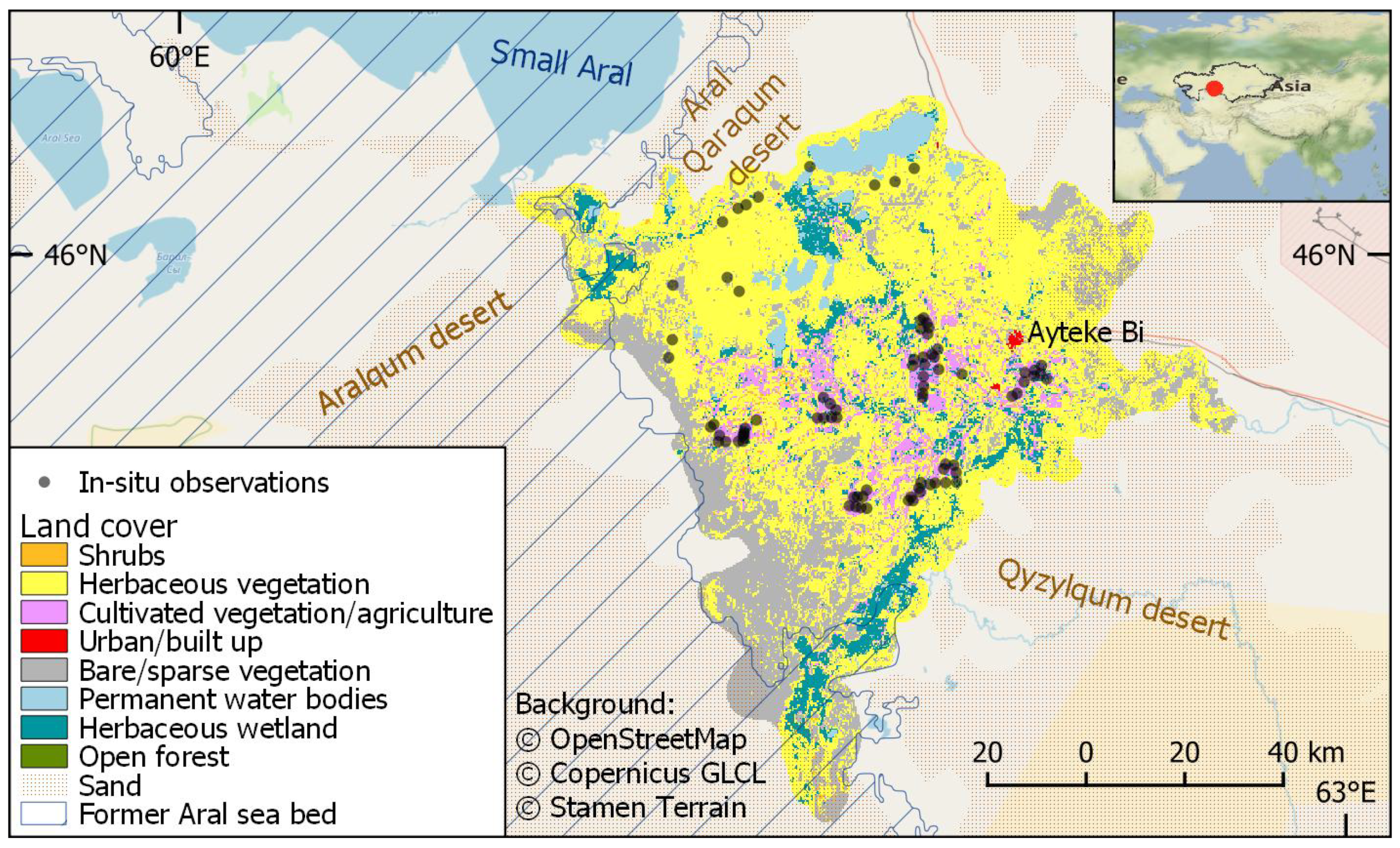
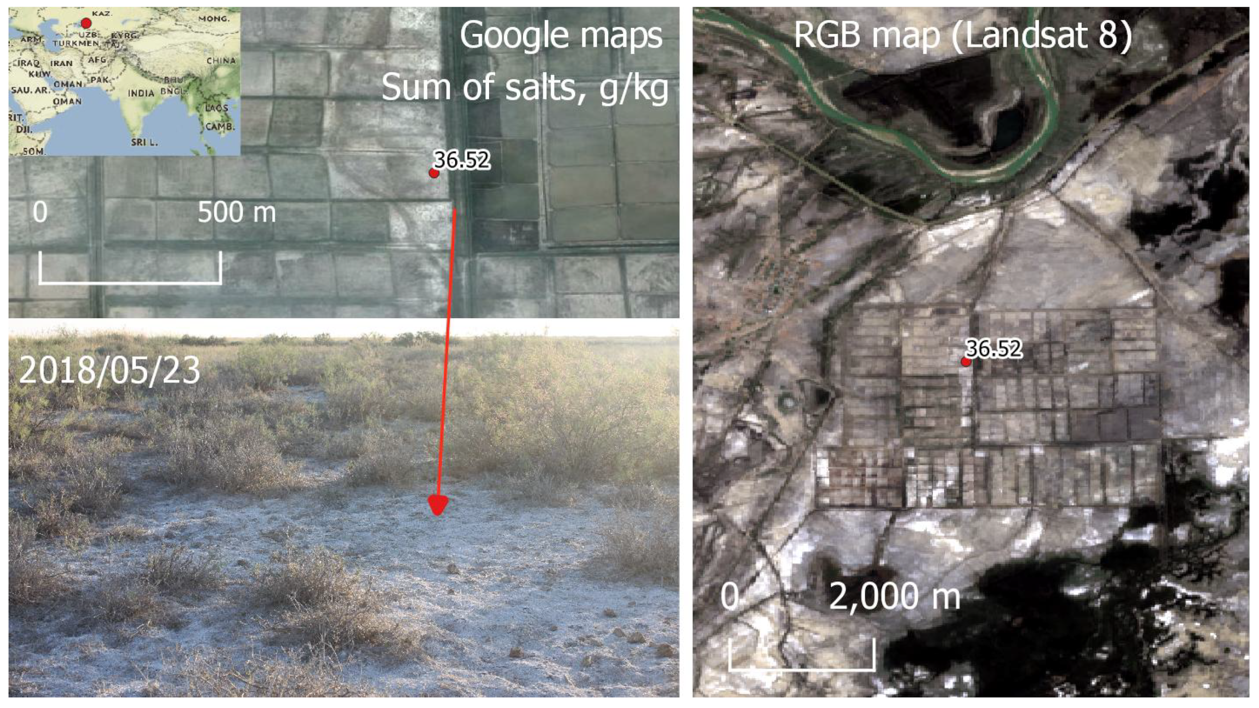
2.1. Description of the Study Area
2.2. The Data and Research Methods
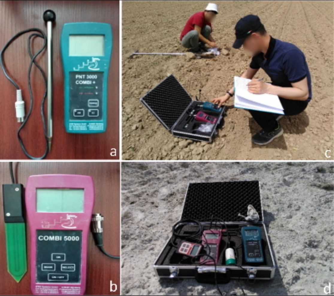
- Field research was conducted once in May 2018, including soil sampling, land cover, and land use observation at 83 locations. The 93 soil samples of the topsoil layer (0–20 cm) and samples at 20–50 cm and 50–100 cm depth were collected (30 samples at each), and soil EC was measured. The coordinates (WGS-84) were measured using the Garmin T650 hand-held global positioning system and a mobile phone with an accuracy of about 10 m due to locations situated primarily in distant areas without a mobile network. The field measurement of the soil electric conductivity (Soil EC) was carried out using the STEP Combi 3000+ device (Figure 3). Pictures of landscapes and vegetation were taken at each location. The field measurements included the soil temperature and moisture measurements using the portable STEP Combi 5000 tool (Germany).
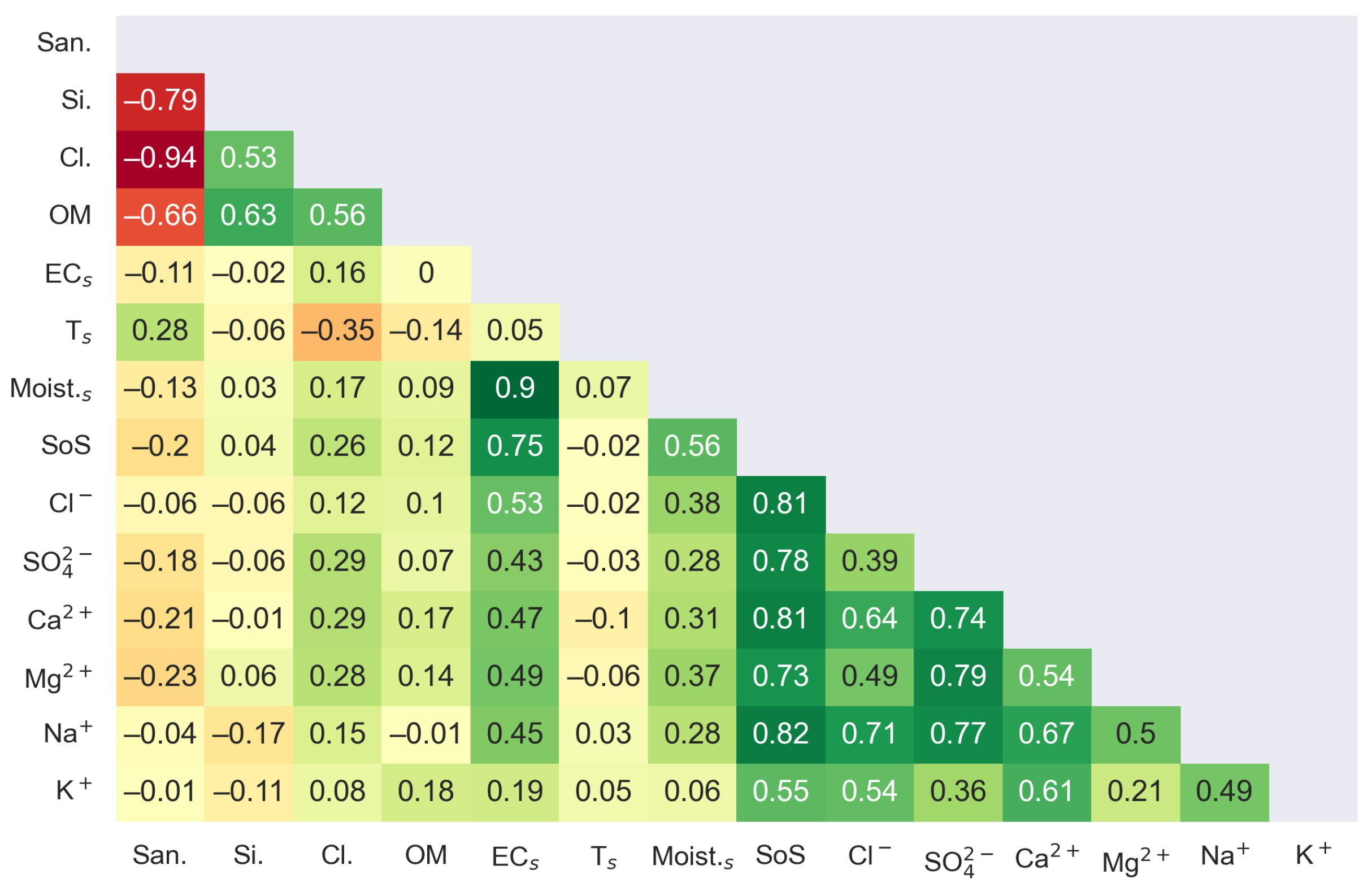
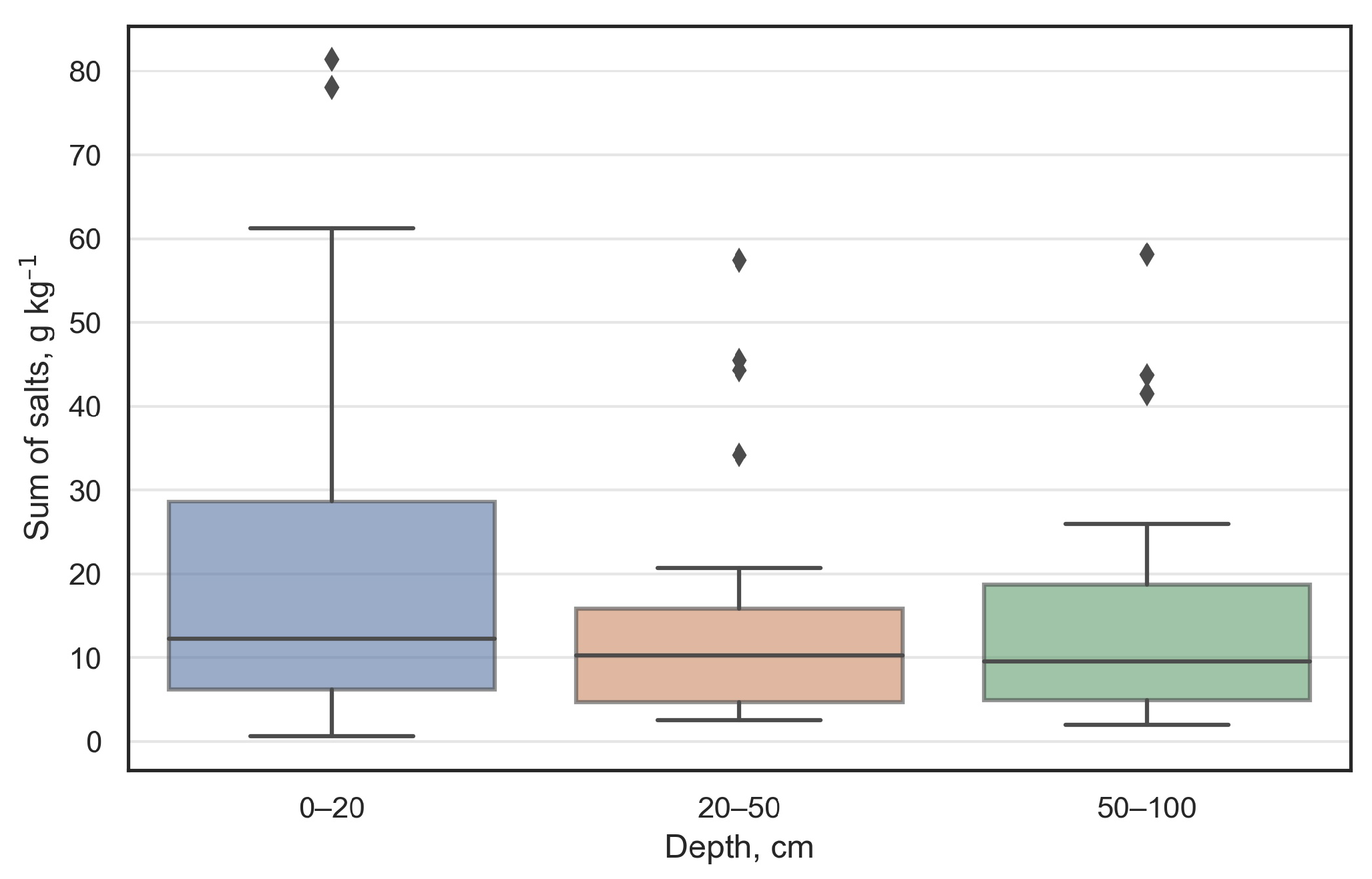
- Data consisting of 14 parameters (sand content (%, Sa.), clay content (%, Cl.), soil organic matter (%, OM-Humus), electric conductivity (dS m, EC), soil temperature (°C, T), soil moisture (mm, Moist), a sum of salt in the soil (g kg, SoS), chlorine (Cl), sulfate (SO), calcium (Ca), magnesium (Mg), sodium (Na), and potassium (K)) were prepossessed to test possible interconnections of variables and to find predictors of the soil salinity expressed by soil electric conductivity. The soil moisture was selected as a potential predictor for the soil salinity, and its correlation with the satellite remote sensing data was tested afterward. The coefficient of determination for selected predictors in the sum of salt in the soil of the medium (20–50 cm) and the lowest (50–100 cm) soil layers did not exceed 0.6; data on the two layers were not included in further modeling. The coordinates of points were checked accurately, and data refinement resulted in a topsoil layer dataset consisting of variables on 31 points (Table 1) out of the initial 93. The sum of salts contains the sum of ions and is included in the table.
- For the physical and chemical analysis, soil samples were transported to the U.U.Uspanov Kazakh Research Institute of Soil Science and Agrochemistry (Almaty, Kazakhstan) for further laboratory analysis. The analysis included several soil parameters: the water hood, mechanical content analysis, electric conductivity, and soil humus content. The soil electrical conductivity was measured using electrodes in an aqueous solution (with distilled water) with a 1:5 ratio (soil: water).
- The Pearson’s coefficient was calculated to characterize the connections between measured parameters according to the equation below.where n is sample size, , are the individual sample points indexed with i, , and is the sample means that is estimated as follows:where is mean value for all values of x, and the equation for y is the same.
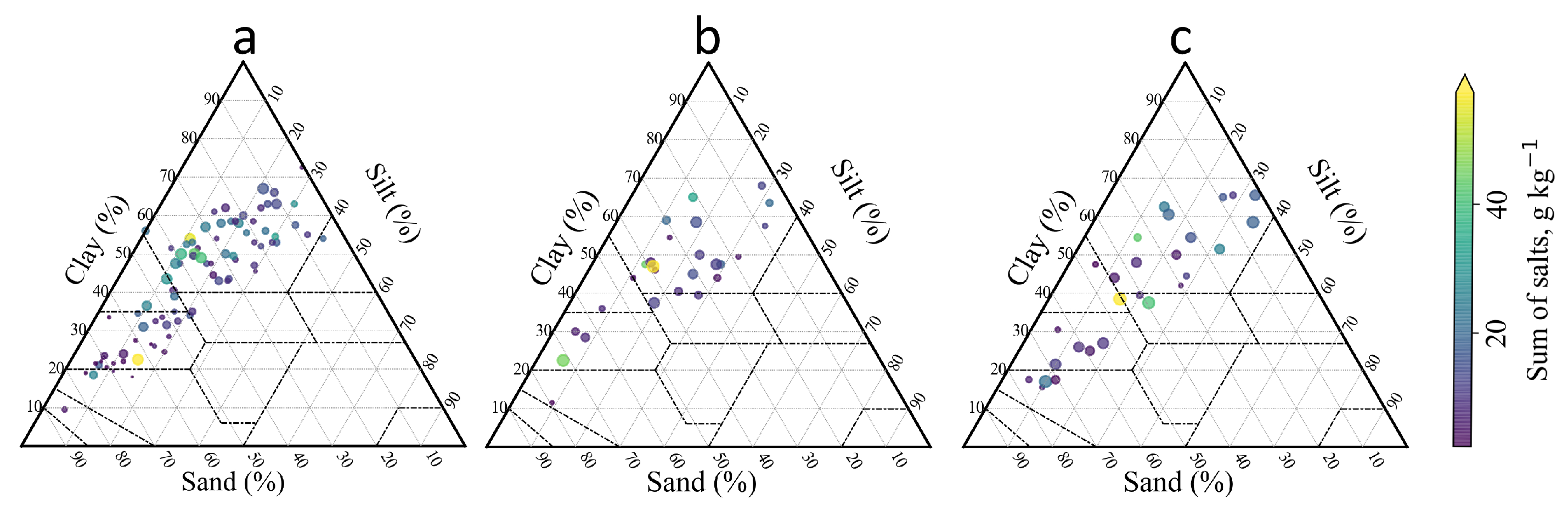
- Soil texture was classified by soil mechanical content data derived after the laboratory analysis according to the USDA classification, and its repetition was also analyzed [66]. The open-source Python software tool Soiltexture 1.0.4 (https://pypi.org/project/soiltexture/ (accessed on 21 September 2022)) was applied for this purpose. To visualize the soil clusters for the study area, the texture triangle [67] implemented through the Python tool SoilTriangle (https://github.com/mishagrol/SoilTriangle (accessed on 21 September 2022)) was used. In the next step, the distribution of the sum of salt in the soil and other parameters within soil texture classes were checked. Soil salt chemical content analysis was also performed to describe the soil salinization.
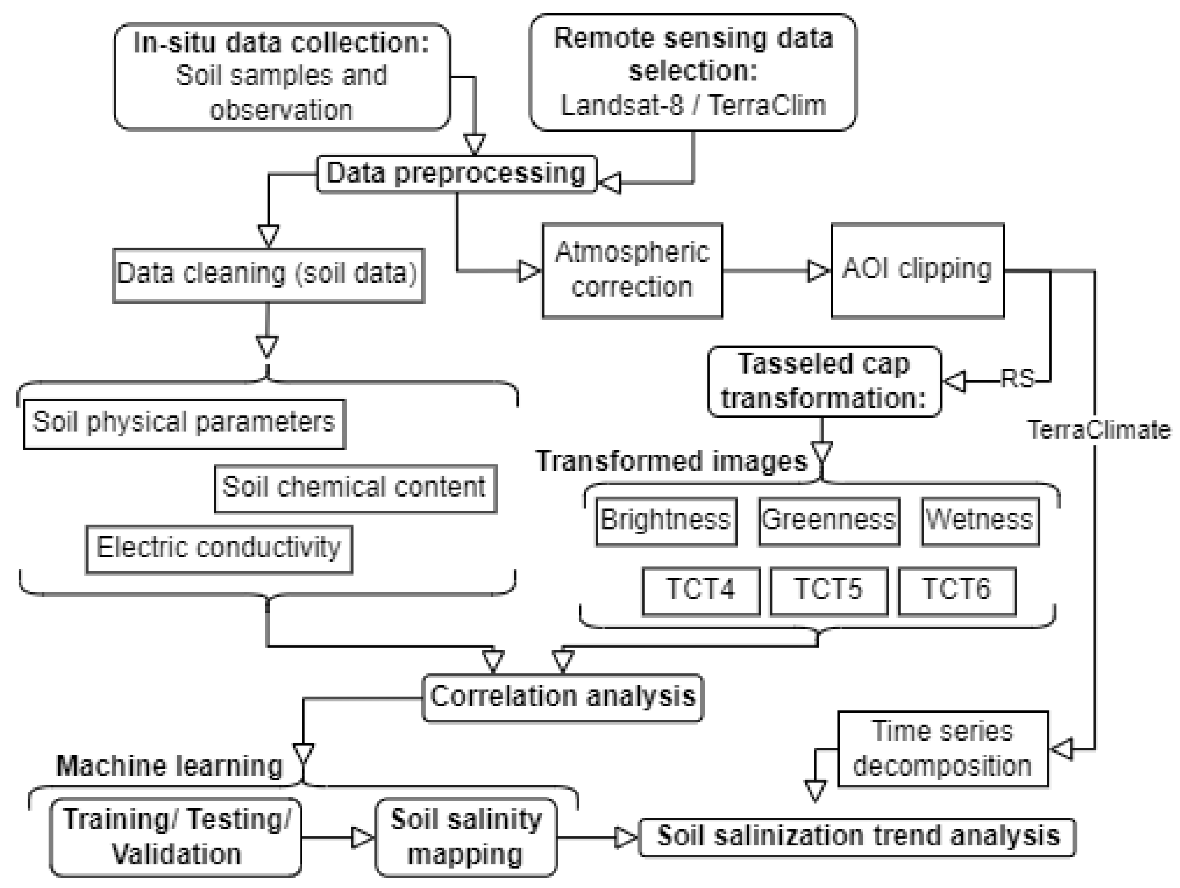
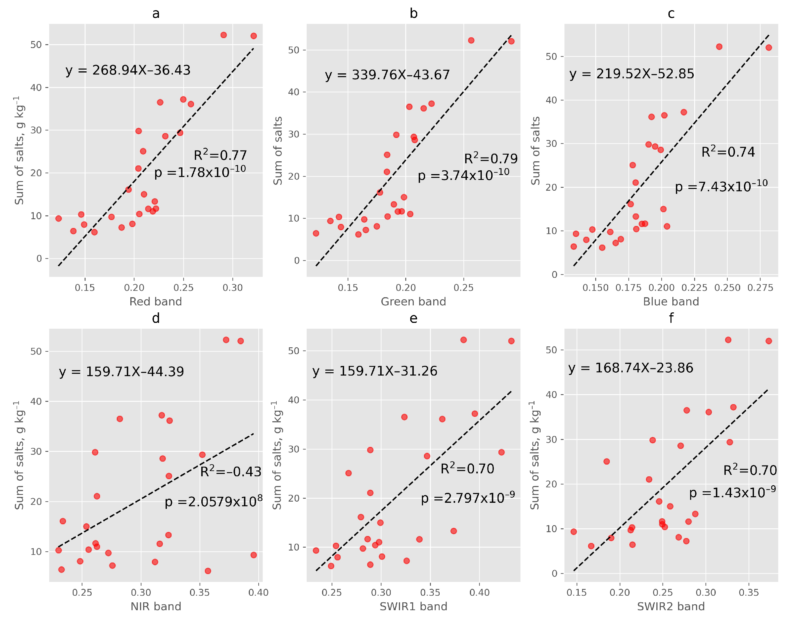
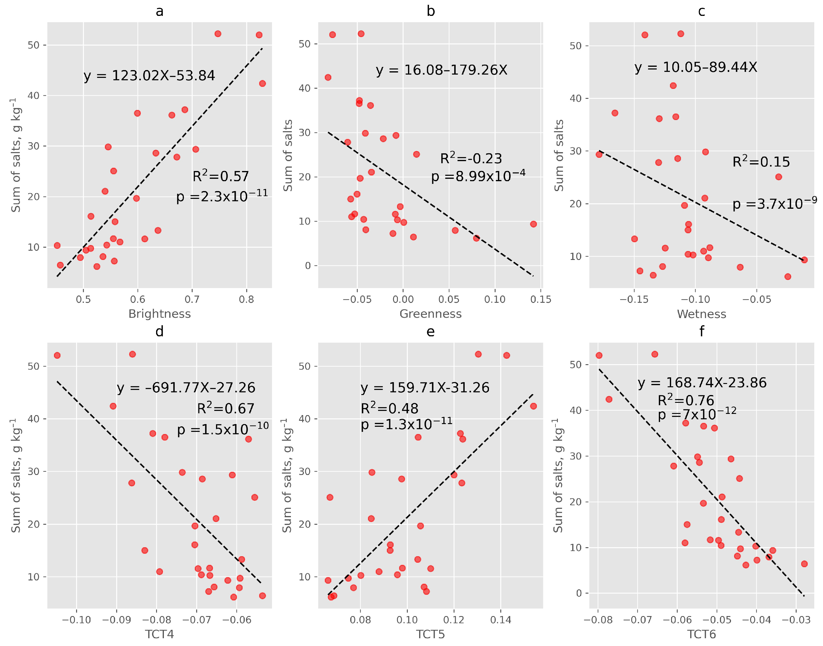
- Tasseled cap transformation was applied to Landsat-8 bands, and 6 coefficients (placed in 6 bands) that improved reflectance of vegetation, soil, and water: greenness, wetness, and brightness, were obtained as coefficients from 4 to 6. These coefficients successfully differentiate soil from vegetation, and in this study, it was decided to apply them to obtain soil information. The values were proposed by Baig et al. [68].The single scene acquired by Landsat-8 (Collection 2 Tier 1 calibrated top-of-atmosphere (TOA) reflectance) was selected for the Qazaly cropping zone to test the possible relationships between the soil salinity and Landsat 8 bands acquired on 13 May 2018 (path 160, row 028). The Google Earth Engine (https://developers.google.com/earth-engine/guides/arrays_array_images (accessed on 20 September 2022)) web service was used to derive the Tasseled Cap Transformed coefficients. Correlation tests of derived TCT coefficients and soil salinity features of the study area were used to define best-matching predictors.
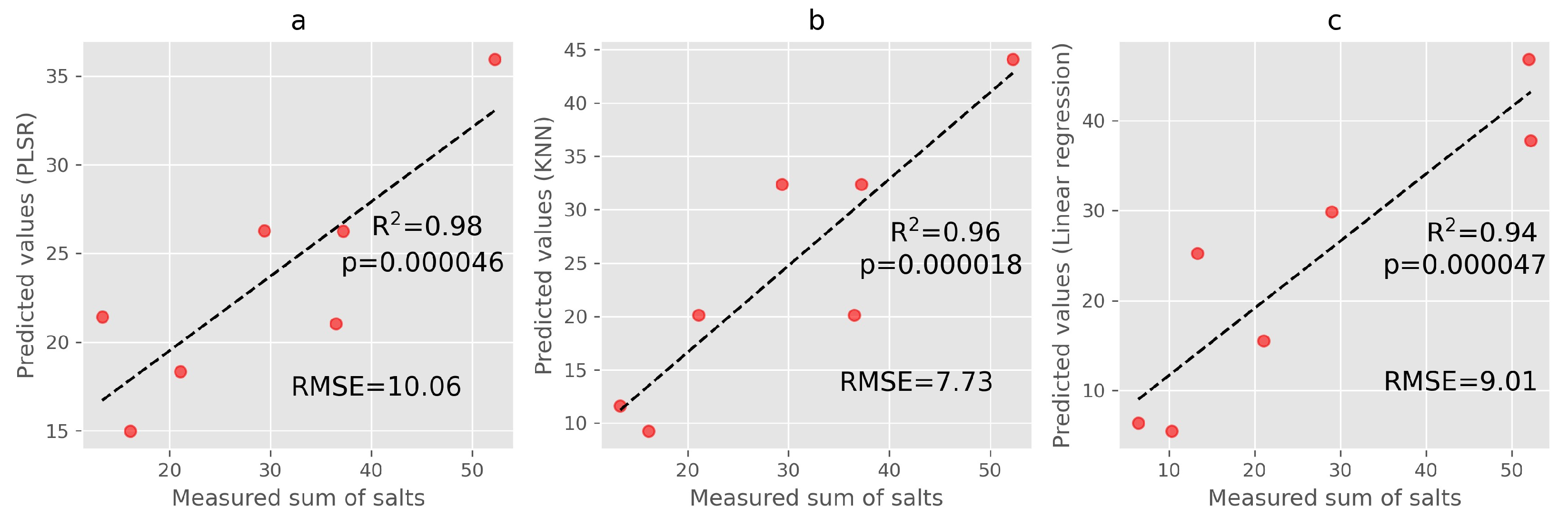
- The soil salinity prediction modeling was built after selecting its predictors. The input dataset, consisting of variables on 31 samples, was established. Due to the high variance of other measurements, the sum of salts in the soil was used. Images acquired on 13 May 2018, 16 July 2018, 2 September 2018, 18 September 2018, and 20 October 2018 were selected for modeling.Three machine learning techniques were chosen to analyze the observed sum of salt in the soil: multiple linear regression (MLR), polynomial regression, K-nearest neighborhood (KNN), and the partial least squares regression (PLSR) for this purpose [35,69,70]. Conditions of using a small yet valuable dataset were similar: the share of train and test values was 70% and 30% within 31 samples. Machine learning open-source Scikit-learn software was used for a regression [71].After this comparison, applying the K-nearest neighbor model to predict soil salinity using Landsat-8 images was decided. It is based on k nearest neighbor for input points, is calculated using the distance between values as the weight in this research, and is expressed using Equation (3):where x is an input band value, and y is the sum of salt in the soil.
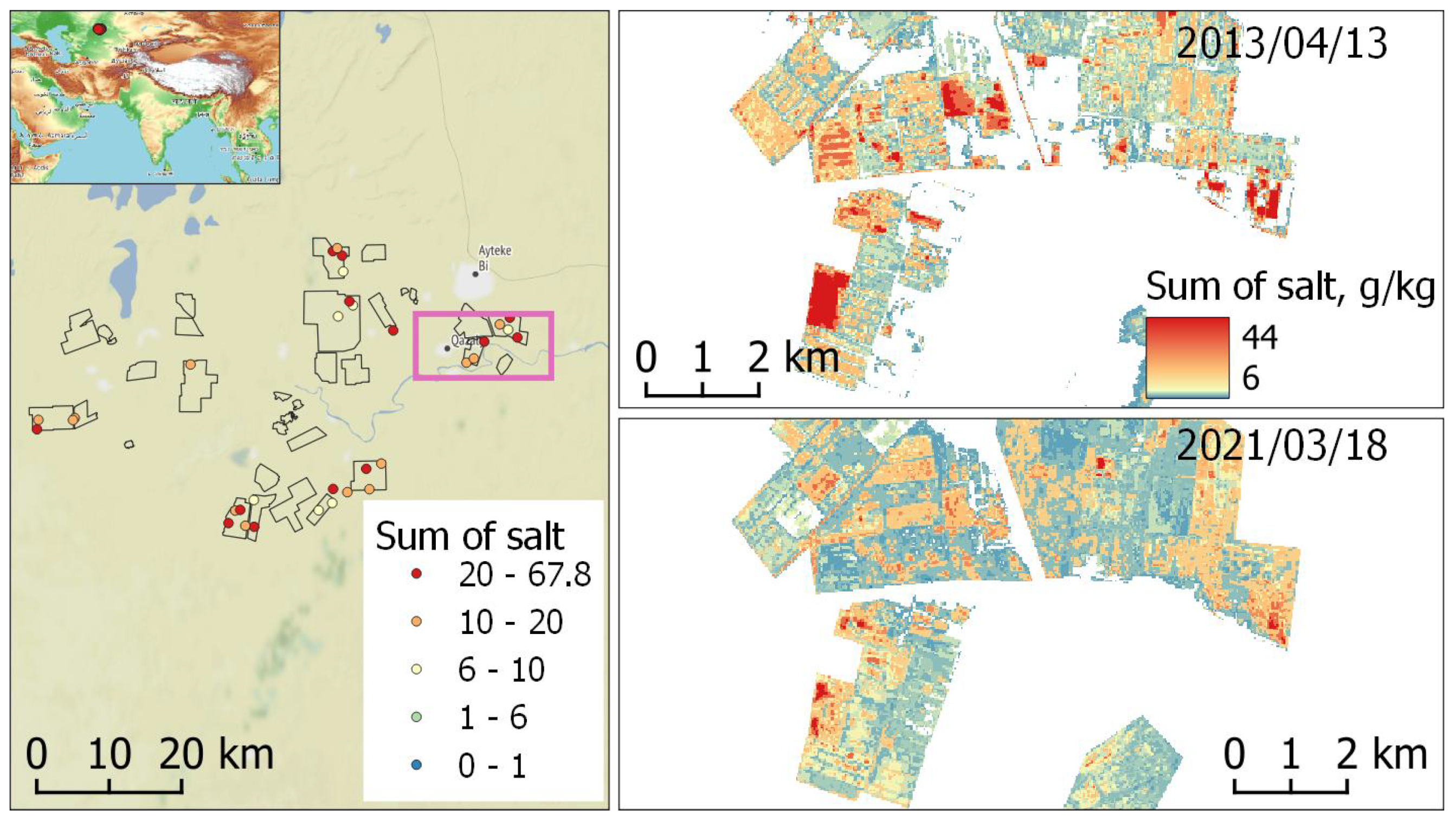
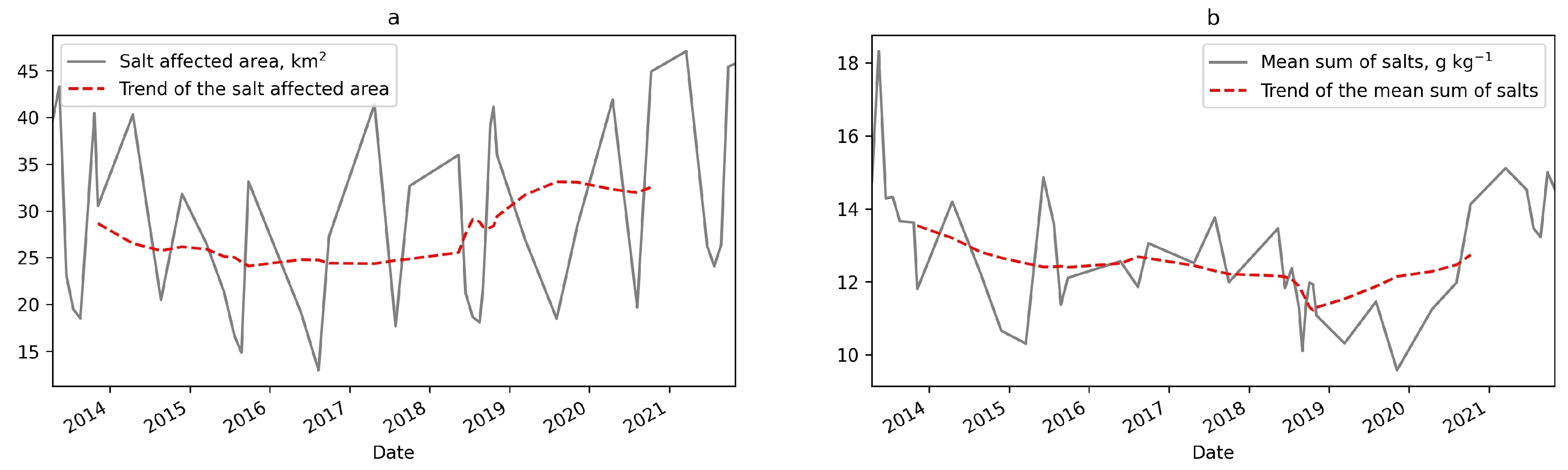
- The quantitative soil salinity assessment for 2013–2021 was performed by applying the regression K-nearest neighbor model. The pixel-wise sum of salt in the soil was derived over 42 periods and calculated for the study area’s croplands. Then, the areas affected by soil salinity were measured and added to the table. Data on the sum of salt in the soil was organized as a set of time series. Trends and seasonal variations of derived parameters were calculated using an additive decomposition model via Python Statsmodel tool (https://www.statsmodels.org/stable/index.html (accessed on 27 September 2022)). The additive model can be described by Equation (4).where is an average value, —increasing/decreasing value, —short-term cycle in the series, —is a random variation, and their summary y is a model of time series.The primary purpose of this study was to set up the proper method and data to quantify soil salinity for the Qazaly irrigation zone using commonly applied satellite image data, and the results are described in the next part.
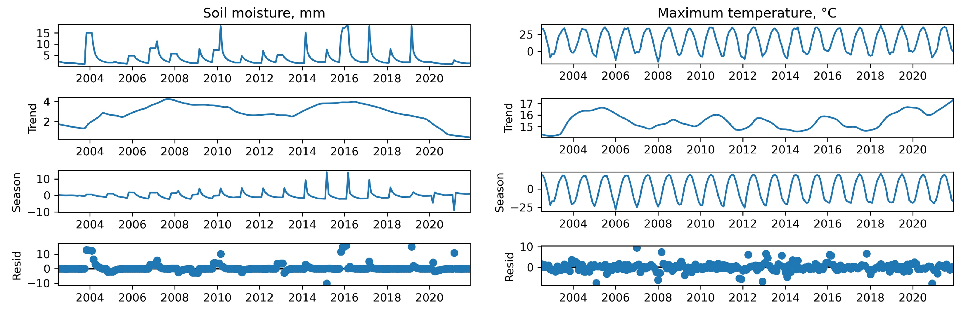
- To monitor the difference in climate change trends, we considered the soil moisture and maximum temperature data by TerraClimate between July 2002 and December 2021 [72]. TerraClimate is a global dataset of the monthly surface climate and water balance. It uses the interpolation method to calculate the data. Thus, we applied the Mann–Kendall test to derive the trends in the soil moisture and maximum temperature at 2 different points for comparison: the first located at the study area (N45.591, E61.9065) and the second at the upper part down to the southern region in the border zone between Kazakhstan and Uzbekistan (N40.88593, E68.092595). Points were selected due to the soil salinity conditions based on the field studies in 2018. We applied the results on the salt-affected soil areas from the previous part to compare the climatic parameters and found several concurrences for the Qazaly irrigation zone.
3. Results
3.1. Statistic Processing of the Field Data
3.2. Distribution of Soil Texture and Salt Chemical Composition
3.3. Selection of Predictors for Soil Salinity Assessment
3.4. The Soil Salinity Modeling
3.5. The Soil Salinization at Croplands
3.6. Soil Salinity and Climate Change
4. Discussion
5. Conclusions
Author Contributions
Funding
Institutional Review Board Statement
Informed Consent Statement
Data Availability Statement
Acknowledgments
Conflicts of Interest
References
- Blaikie, P.; Brookfield, H. Land Degradation and Society; Routledge: London, UK, 2015. [Google Scholar]
- Metternicht, G.I.; Zinck, J.A. Remote sensing of soil salinity: Potentials and constraints. Remote Sens. Environ. 2003, 85, 1–20. [Google Scholar] [CrossRef]
- Montanarella, L.; Pennock, D.J.; McKenzie, N.; Badraoui, M.; Chude, V.; Baptista, I.; Mamo, T.; Yemefack, M.; Aulakh, M.S.; Yagi, K.; et al. World’s soils are under threat. Soil 2016, 2, 79–82. [Google Scholar] [CrossRef]
- Hussain, Z.; Khattak, R.A.; Fareed, I.; Irshad, M.; Mahmood, Q. Interaction of Phosphorus and Potassium on Maize (Zea mays L.) in Saline-Sodic Soil. J. Agric. Sci. 2015, 7, 66–78. [Google Scholar] [CrossRef]
- Ivushkin, K.; Bartholomeus, H.; Bregt, A.K.; Pulatov, A.; Kempen, B.; de Sousa, L. Global mapping of soil salinity change. Remote Sens. Environ. 2019, 231, 111260. [Google Scholar] [CrossRef]
- Singh, A. Soil salinity: A global threat to sustainable development. Soil Use Manag. 2022, 38, 39–67. [Google Scholar] [CrossRef]
- Mukhopadhyay, R.; Sarkar, B.; Jat, H.S.; Sharma, P.C.; Bolan, N.S. Soil salinity under climate change: Challenges for sustainable agriculture and food security. J. Environ. Manag. 2021, 280, 111736. [Google Scholar] [CrossRef]
- Bissenbayeva, S.; Abuduwaili, J.; Saparova, A.; Ahmed, T. Long-term variations in runoff of the Syr Darya River Basin under climate change and human activities. J. Arid. Land 2021, 13, 56–70. [Google Scholar] [CrossRef]
- Eswar, D.; Karuppusamy, R.; Chellamuthu, S. Drivers of soil salinity and their correlation with climate change. Curr. Opin. Environ. Sustain. 2021, 50, 310–318. [Google Scholar] [CrossRef]
- Niedrist, G.H.; Psenner, R.; Sommaruga, R. Climate warming increases vertical and seasonal water temperature differences and inter-annual variability in a mountain lake. Clim. Chang. 2018, 151, 473–490. [Google Scholar] [CrossRef]
- Qi, X.; Jia, J.; Liu, H.; Lin, Z. Relative importance of climate change and human activities for veobtaination changes on China’s silk road economic belt over multiple timescales. Catena 2019, 180, 224–237. [Google Scholar] [CrossRef]
- Venkatesh, K.; John, R.; Chen, J.; Jarchow, M.; Amirkhiz, R.G.; Giannico, V.; Saraf, S.; Jain, K.; Kussainova, M.; Yuan, J. Untangling the impacts of socioeconomic and climatic changes on veobtaination greenness and productivity in Kazakhstan. Environ. Res. Lett. 2022, 17, 095007. [Google Scholar] [CrossRef]
- Halsch, C.A.; Shapiro, A.M.; Fordyce, J.A.; Nice, C.C.; Thorne, J.H.; Waetjen, D.P.; Forister, M.L. Insects and recent climate change. Proc. Natl. Acad. Sci. USA 2021, 118, e2002543117. [Google Scholar] [CrossRef] [PubMed]
- Zare, E.; Huang, J.; Santos, F.M.; Triantafilis, J. Mapping salinity in three dimensions using a DUALEM-421 and electromagnetic inversion software. Soil Sci. Soc. Am. J. 2015, 79, 1729–1740. [Google Scholar] [CrossRef]
- Zhao, D.; Li, N.; Zare, E.; Wang, J.; Triantafilis, J. Mapping cation exchange capacity using a quasi-3d joint inversion of EM38 and EM31 data. Soil Tillage Res. 2020, 200, 104618. [Google Scholar] [CrossRef]
- Zhao, D.; Wang, J.; Zhao, X.; Triantafilis, J. Clay content mapping and uncertainty estimation using weighted model averaging. Catena 2022, 209, 105791. [Google Scholar] [CrossRef]
- Allbed, A.; Kumar, L. Soil salinity mapping and monitoring in arid and semi-arid regions using remote sensing technology: A review. Adv. Remote. Sens. 2013, 2013, 41262. [Google Scholar] [CrossRef]
- Gorji, T.; Sertel, E.; Tanik, A. Monitoring soil salinity via remote sensing technology under data scarce conditions: A case study from Turkey. Ecol. Indic. 2017, 74, 384–391. [Google Scholar] [CrossRef]
- Ben-Dor, E. Quantitative remote sensing of soil properties. Adv. Agron. 2002, 75, 173–243. [Google Scholar] [CrossRef]
- Dehaan, R.; Taylor, G. Image-derived spectral endmembers as indicators of salinisation. Int. J. Remote. Sens. 2003, 24, 775–794. [Google Scholar] [CrossRef]
- Howari, F. The use of remote sensing data to extract information from agricultural land with emphasis on soil salinity. Soil Res. 2003, 41, 1243–1253. [Google Scholar] [CrossRef]
- Farifteh, J.; Farshad, A.; George, R. Assessing salt-affected soils using remote sensing, solute modeling, and geophysics. Geoderma 2006, 130, 191–206. [Google Scholar] [CrossRef]
- Farifteh, J.; Van der Meer, F.; Atzberger, C.; Carranza, E. Quantitative analysis of salt-affected soil reflectance spectra: A comparison of two adaptive methods (PLSR and ANN). Remote Sens. Environ. 2007, 110, 59–78. [Google Scholar] [CrossRef]
- Wang, L.; Qu, J.J. NMDI: A normalized multi-band drought index for monitoring soil and veobtaination moisture with satellite remote sensing. Geophys. Res. Lett. 2007, 34. [Google Scholar] [CrossRef]
- Metternicht, G.; Zinck, A. Remote Sensing of Soil Salinization: Impact on Land Management; CRC Press: Boca Raton, FL, USA, 2008. [Google Scholar]
- Ben-Dor, E.; Chabrillat, S.; Demattê, J.A.M.; Taylor, G.; Hill, J.; Whiting, M.; Sommer, S. Using imaging spectroscopy to study soil properties. Remote Sens. Environ. 2009, 113, S38–S55. [Google Scholar] [CrossRef]
- Ozdogan, M.; Yang, Y.; Allez, G.; Cervantes, C. Remote sensing of irrigated agriculture: Opportunities and challenges. Remote Sens. 2010, 2, 2274–2304. [Google Scholar] [CrossRef]
- Sidike, A.; Zhao, S.; Wen, Y. Estimating soil salinity in Pingluo County of China using QuickBird data and soil reflectance spectra. Int. J. Appl. Earth Obs. Geoinf. 2014, 26, 156–175. [Google Scholar] [CrossRef]
- Bai, L.; Wang, C.; Zang, S.; Zhang, Y.; Hao, Q.; Wu, Y. Remote sensing of soil alkalinity and salinity in the Wuyu’er-Shuangyang river basin, Northeast China. Remote Sens. 2016, 8, 163. [Google Scholar] [CrossRef]
- Bannari, A.; El-Battay, A.; Bannari, R.; Rhinane, H. Sentinel-MSI VNIR and SWIR bands sensitivity analysis for soil salinity discrimination in an arid landscape. Remote Sens. 2018, 10, 855. [Google Scholar] [CrossRef]
- Jiang, H.; Shu, H. Optical remote-sensing data based research on detecting soil salinity at different depth in an arid-area oasis, Xinjiang, China. Earth Sci. Inform. 2019, 12, 43–56. [Google Scholar] [CrossRef]
- Goehring, N.; Verburg, P.; Saito, L.; Jeong, J.; Meki, M.N. Improving modeling of quinoa growth under saline conditions using the enhanced agricultural policy environmental extender model. Agronomy 2019, 9, 592. [Google Scholar] [CrossRef]
- Abuelgasim, A.; Ammad, R. Mapping soil salinity in arid and semi-arid regions using Landsat 8 OLI satellite data. Remote Sens. Appl. Soc. Environ. 2019, 13, 415–425. [Google Scholar] [CrossRef]
- Nguyen, K.A.; Liou, Y.A.; Tran, H.P.; Hoang, P.P.; Nguyen, T.H. Soil salinity assessment by using near-infrared channel and Veobtaination Soil Salinity Index derived from Landsat 8 OLI data: A case study in the Tra Vinh Province, Mekong Delta, Vietnam. Prog. Earth Planet. Sci. 2020, 7, 1. [Google Scholar] [CrossRef]
- Wang, J.; Peng, J.; Li, H.; Yin, C.; Liu, W.; Wang, T.; Zhang, H. Soil Salinity Mapping Using Machine Learning Algorithms with the Sentinel-2 MSI in Arid Areas, China. Remote Sens. 2021, 13, 305. [Google Scholar] [CrossRef]
- Drusch, M.; Del Bello, U.; Carlier, S.; Colin, O.; Fernandez, V.; Gascon, F.; Hoersch, B.; Isola, C.; Laberinti, P.; Martimort, P.; et al. Sentinel-2: ESA’s Optical High-Resolution Mission for GMES Operational Services. Remote Sens. Environ. 2012, 120, 25–36. [Google Scholar] [CrossRef]
- Irons, J.R.; Dwyer, J.L.; Barsi, J.A. The next Landsat satellite: The Landsat Data Continuity Mission. Remote Sens. Environ. 2012, 122, 11–21. [Google Scholar] [CrossRef]
- Crétaux, J.F.; Biancamaria, S.; Arsen, A.; Bergé Nguyen, M.; Becker, M. Global surveys of reservoirs and lakes from satellites and regional application to the Syrdarya river basin. Environ. Res. Lett. 2015, 10, 015002. [Google Scholar] [CrossRef]
- Beck, R.; Xu, M.; Zhan, S.; Liu, H.; Johansen, R.A.; Tong, S.; Yang, B.; Shu, S.; Wu, Q.; Wang, S.; et al. Comparison of satellite reflectance algorithms for estimating phycocyanin values and cyanobacterial total biovolume in a temperate reservoir using coincident hyperspectral aircraft imagery and dense coincident surface observations. Remote Sens. 2017, 9, 538. [Google Scholar] [CrossRef]
- Kussul, N.; Mykola, L.; Shelestov, A.; Skakun, S. Crop inventory at regional scale in Ukraine: Developing in season and end of season crop maps with multi-temporal optical and SAR satellite imagery. Eur. J. Remote. Sens. 2018, 51, 627–636. [Google Scholar] [CrossRef]
- Morgan, R.S.; El-Hady, M.A.; Rahim, I.S. Soil salinity mapping utilizing sentinel-2 and neural networks. Indian J. Agric. Res. 2018, 52, 524–529. [Google Scholar] [CrossRef]
- Hihi, S.; Rabah, Z.B.; Bouaziz, M.; Chtourou, M.Y.; Bouaziz, S. Prediction of Soil Salinity Using Remote Sensing Tools and Linear Regression Model. Adv. Remote Sens. 2019, 08, 77–88. [Google Scholar] [CrossRef]
- Bannari, A.; Al-Ali, Z.M. Assessing climate change impact on soil salinity dynamics between 1987–2017 in arid landscape using Landsat TM, ETM+ and OLI data. Remote Sens. 2020, 12, 2794. [Google Scholar] [CrossRef]
- Jollife, I.T.; Cadima, J. Principal component analysis: A review and recent developments. Philos. Trans. R. Soc. Math. Phys. Eng. Sci. 2016, 374, 20150202. [Google Scholar] [CrossRef] [PubMed]
- Lamqadem, A.A.; Saber, H.; Pradhan, B. Quantitative assessment of desertification in an arid oasis using remote sensing data and spectral index techniques. Remote Sens. 2018, 10, 1862. [Google Scholar] [CrossRef]
- Löw, F.; Conrad, C.; Michel, U. Decision fusion and non-parametric classifiers for land use mapping using multi-temporal RapidEye data. Isprs J. Photogramm. Remote Sens. 2015, 108, 191–204. [Google Scholar] [CrossRef]
- Ivushkin, K.; Bartholomeus, H.; Bregt, A.K.; Pulatov, A. Satellite thermography for soil salinity assessment of cropped areas in Uzbekistan. Land Degrad. Dev. 2017, 28, 870–877. [Google Scholar] [CrossRef]
- Vyrakhmanova, A.; Otarov, A.; Saparov, A.; Suska-Malavska, M.; Duisekov, S.; Poshanov, M.; Tanirbergenov, S. The ecological status of irrigated saline soils of the Shaulder massif of the Turkestan region. Eurasian J. Biosci. 2020, 14, 347–354. [Google Scholar]
- Kotlyakov, V.M. The Aral Sea basin: A critical environmental zone. Environ. Sci. Policy Sustain. Dev. 1991, 33, 4–38. [Google Scholar] [CrossRef]
- Kosaki, T.; Suzuki, R.; Ishida, N.; Funakawa, S. Salt-Affected Soils under Large-Scale Irrigation Agriculture in Kazakhstan. In Forum on the Caspian, Aral and Dead Seas: Perspectives of Water Environment Management and Politics. Symposium onthe Aral Sea and Surrounding Region; UNEP International Environmental Technology Centre: Osaka, Japan, 1995; Volume 4, p. 136. [Google Scholar]
- Tsutsui, H.; Ogino, Y. Irrigation management for paddy-based agriculture in the deltas of the Aral Sea Basin. J. Irrig. Eng. Rural. Plan. 1995, 1995, 42–51. [Google Scholar]
- Funakawa, S.; Suzuki, R.; Karbozova, E.; Kosaki, T.; Ishida, N. Salt-affected soils under rice-based irrigation agriculture in southern Kazakhstan. Geoderma 2000, 97, 61–85. [Google Scholar] [CrossRef]
- Sugimori, Y.; Funakawa, S.; Pachikin, K.; Ishida, N.; Kosaki, T. Soil salinity dynamics in irrigated fields and its effects on paddy-based rotation systems in southern Kazakhstan. Land Degrad. Dev. 2008, 19, 305–320. [Google Scholar] [CrossRef]
- Pachikin, K.; Erokhina, O.; Funakawa, S. Properties and distribution pattern of soils in Kazakhstan. Pedologist 2009, 53, 30–37. [Google Scholar]
- Saparov, A. Soil resources of the Republic of Kazakhstan: Current status, problems and solutions. In Novel Measurement and Assessment Tools for Monitoring and Management of Land and Water Resources in Agricultural Landscapes of Central Asia; Springer: Berlin/Heidelberg, Germany, 2014; pp. 61–73. [Google Scholar]
- Umbetaev, I.; Bigaraev, O.; Baimakhanov, K. Effect of soil salinity on the yield of cotton in Kazakhstan. Russ. Agric. Sci. 2015, 41, 222–224. [Google Scholar] [CrossRef]
- Issanova, G.T.; Abuduwaili, J.; Mamutov, Z.U.; Kaldybaev, A.A.; Saparov, G.A.; Bazarbaeva, T.A. Saline soils and identification of salt accumulation provinces in Kazakhstan. Arid Ecosyst. 2017, 7, 243–250. [Google Scholar] [CrossRef]
- Bekbayev, R.; Balgabayev, N.; Zhaparkulova, Y.; Karlihanov, O.; Musin, Z. Factors that intensify soil degradation in the Kazakhstan part of the Golodnostepsky irrigation massif. Life Sci. J. 2015, 97, 194–200. [Google Scholar]
- Laiskhanov, S.U.; Otarov, A.; Savin, I.Y.; Tanirbergenov, S.I.; Mamutov, Z.U.; Duisekov, S.N.; Zhogolev, A. Dynamics of soil salinity in irrigation areas in South Kazakhstan. Polish J. Environ. Stud. 2016, 25, 2469–2476. [Google Scholar] [CrossRef]
- Duan, Y.; Ma, L.; Abuduwaili, J.; Liu, W.; Saparov, G. Driving Factor Identification for the Spatial Distribution of Soil Salinity in the Irrigation Area of the Syr Darya River, Kazakhstan. Agronomy 2022, 12, 1912. [Google Scholar] [CrossRef]
- Liu, W.; Ma, L.; Smanov, Z.; Samarkhanov, K.; Abuduwaili, J. Clarifying Soil Texture and Salinity Using Local Spatial Statistics (Getis-Ord Gi* and Moran’s I) in Kazakh–Uzbekistan Border Area, Central Asia. Agronomy 2022, 12, 332. [Google Scholar] [CrossRef]
- Jin, Q.; Wei, J.; Yang, Z.L.; Lin, P. Irrigation-Induced Environmental Changes around the Aral Sea: An Integrated View from Multiple Satellite Observations. Remote Sens. 2017, 9, 900. [Google Scholar] [CrossRef]
- Jiang, L.; Jiapaer, G.; Bao, A.; Guo, H.; Ndayisaba, F. Veobtaination dynamics and responses to climate change and human activities in Central Asia. Sci. Total Environ. 2017, 599–600, 967–980. [Google Scholar] [CrossRef]
- Tukey, J.W. Exploratory Data Analysis; Pearson: Reading, MA, USA, 1977; Volume 2. [Google Scholar]
- Dawson, R. How significant is a boxplot outlier? J. Stat. Educ. 2011, 19. [Google Scholar] [CrossRef]
- Yang, J.; Guan, X.; Luo, M.; Wang, T. Cross-system legacy data applied to digital soil mapping: A case study of Second National Soil Survey data in China. Geoderma Reg. 2022, 28, e00489. [Google Scholar] [CrossRef]
- Groenendyk, D.G.; Ferré, T.P.; Thorp, K.R.; Rice, A.K. Hydrologic-process-based soil texture classifications for improved visualization of landscape function. PLoS ONE 2015, 10, e131299. [Google Scholar] [CrossRef] [PubMed]
- Baig, M.H.A.; Zhang, L.; Shuai, T.; Tong, Q. Derivation of a tasselled cap transformation based on Landsat 8 at-satellite reflectance. Remote Sens. Lett. 2014, 5, 423–431. [Google Scholar] [CrossRef]
- Azabdaftari, A.; Sunar, F. Soil salinity mapping using multitemporal landsat data. Int. Arch. Photogramm. Remote. Sens. Spat. Inf. Sci. ISPRS Arch. 2016, 41, 3–9. [Google Scholar] [CrossRef]
- Yan, J.; Han, L.; Qian, Y.; Zhou, W.; Li, W. Comparing Machine Learning Classifiers for Object-Based Land Cover Classification Using Very High Resolution Imagery. Remote Sens. 2014, 7, 153–168. [Google Scholar] [CrossRef]
- Hakim. Clustering a Satellite Image with Scikit-Learn. 2018. Available online: https://medium.com/@h4k1m0u/clustering-a-satellite-image-with-scikit-learn-14adb2ca3790 (accessed on 22 September 2022).
- Abatzoglou, J.T.; Dobrowski, S.Z.; Parks, S.A.; Hegewisch, K.C. TerraClimate, a high-resolution global dataset of monthly climate and climatic water balance from 1958–2015. Sci. Data 2018, 5, 1–12. [Google Scholar] [CrossRef]
- Yang, Y.; Shen, Q.; Li, J.; Deng, Z.; Wang, H.; Gao, X. Position and attitude estimation method integrating visual odometer and GPS. Sensors 2020, 20, 2121. [Google Scholar] [CrossRef]


| Name | E | N | Sa. | Si. | Cl. | OM | T | Moist | EC | SoS |
|---|---|---|---|---|---|---|---|---|---|---|
| S103 | 45.68 | 61.4 | 34.5 | 18 | 47.5 | 0.97 | 32.9 | 8.6 | 0.49 | 16.77 |
| S108 | 45.68 | 61.4 | 34 | 23 | 43 | 1.56 | 39.3 | 15.6 | 5.58 | 17.01 |
| S113 | 45.68 | 61.4 | 17 | 30 | 53 | 1.18 | 42 | 8.6 | 1.23 | 11.66 |
| S134 | 45.9 | 61.3 | 44 | 0 | 56 | 1.11 | 39.7 | 14.2 | 3.51 | 28.98 |
| S143 | 45.7 | 61.6 | 20 | 20 | 60 | 1.52 | 35.8 | 14.5 | 3.33 | 16.12 |
| S144 | 45.5 | 61.7 | 20 | 28 | 52 | 1.32 | 34 | 7.4 | 1.74 | 15.02 |
| S146 | 45.5 | 61.7 | 23.5 | 18 | 58.5 | 0.93 | 37.5 | 10.4 | 2.96 | 28.6 |
| S147 | 45.5 | 61.8 | 39 | 10 | 51 | 1.04 | 40.5 | 18.1 | 8.51 | 52.03 |
| S149 | 45.6 | 61.7 | 21.5 | 23 | 55.5 | 1.04 | 36.8 | 9.1 | 4.72 | 29.83 |
| S150 | 45.6 | 61.7 | 32 | 25 | 43 | 1.11 | 39.8 | 7.2 | 1.58 | 11.02 |
| S151 | 45.6 | 61.8 | 33.5 | 19 | 47.5 | 1.11 | 36 | 5.1 | 0.42 | 6.17 |
| S152 | 45.6 | 61.9 | 31.5 | 11 | 57.5 | 0.45 | 32.7 | 19.7 | 4.93 | 42.41 |
| S154 | 45.6 | 61.9 | 23 | 15 | 62 | 0.97 | 37.1 | 16.0 | 3.53 | 8.11 |
| S157 | 45.6 | 61.9 | 15 | 23 | 62 | 1 | 33.5 | 9.6 | 1.43 | 9.35 |
| S158 | 45.6 | 61.9 | 36.5 | 11 | 52.5 | 0.41 | 33.2 | 10.8 | 2.62 | 19.67 |
| S160 | 45.6 | 62.0 | 40.5 | 12 | 47.5 | 0.79 | 33.1 | 7.6 | 0.77 | 11.6 |
| S163 | 45.62 | 62.0 | 26 | 13 | 61 | 1.92 | 30.2 | 7.0 | 1.15 | 10.42 |
| S165 | 45.61 | 62.0 | 41.5 | 11 | 47.5 | 0.51 | 27 | 26.6 | 9.91 | 36.52 |
| S167 | 45.8 | 62.0 | 27.5 | 24 | 48.5 | 1.41 | 31.8 | 7.2 | 0.86 | 7.94 |
| S171 | 45.82 | 62.0 | 57 | 17 | 26 | 1.23 | 39.5 | 3.8 | 0.56 | 7.24 |
| S172 | 45.82 | 62.0 | 45 | 21 | 34 | 1.68 | 40.4 | 10.2 | 1.77 | 21.07 |
| S174 | 45.8 | 62.0 | 46 | 15 | 39 | 0.93 | 35.3 | 16.0 | 7.12 | 27.83 |
| S180 | 45.9 | 62.0 | 36.5 | 14 | 49.5 | 0.65 | 39 | 11.8 | 1.22 | 13.31 |
| S181 | 45.9 | 62.0 | 29 | 21 | 50 | 0.65 | 39.8 | 18.4 | 5.12 | 29.37 |
| S183 | 45.8 | 62.0 | 51.5 | 15 | 33.5 | 0.79 | 41.8 | 5.2 | 0.51 | 6.43 |
| S184 | 45.9 | 62.0 | 27.5 | 23 | 49.5 | 1.44 | 41.9 | 12.9 | 4.13 | 37.22 |
| S187 | 45.8 | 62.2 | 21 | 26 | 53 | 1.13 | 45.1 | 6.6 | 2.95 | 9.73 |
| S188 | 45.8 | 62.2 | 53.5 | 10 | 36.5 | 0.38 | 42.7 | 22.6 | 8.61 | 36.13 |
| S189 | 45.8 | 62.2 | 39 | 11 | 50 | 0.75 | 42.7 | 29.9 | 10.87 | 52.24 |
| S191 | 45.8 | 62.2 | 57 | 12 | 31 | 1.06 | 41.3 | 21.6 | 7.68 | 25.08 |
| S192 | 45.7 | 62.1 | 44 | 21 | 35 | 1.89 | 38.9 | 13.1 | 1.01 | 10.31 |
| Soil Mech. Content | Soil Layer Depth, cm | |||
|---|---|---|---|---|
| 0–20 | 50–100 | 20–50 | Total | |
| loamy sand | 1 | 1 | ||
| sandy loam | 4 | 4 | 1 | 9 |
| sandy clay loam | 26 | 6 | 5 | 37 |
| sandy clay | 6 | 3 | 2 | 11 |
| clay loam | 1 | 2 | 2 | 5 |
| clay | 54 | 15 | 20 | 89 |
| silty clay | 1 | 1 | ||
| SO | Cl | Total | |
|---|---|---|---|
| Ca | 111 | 6 | 117 |
| Na | 25 | 11 | 36 |
| Total | 136 | 17 | 153 |
| LandSat-8 TCT | (Blue) Band 2 | (Green) Band 3 | Red Band 4 | NIR Band 5 | SWIR1 Band 6 | SWIR2 Band 7 |
|---|---|---|---|---|---|---|
| Brightness | 0.3029 | 0.2786 | 0.4733 | 0.5599 | 0.508 | 0.1872 |
| Greenness | −0.2941 | −0.243 | −0.5424 | 0.7276 | 0.0713 | −0.1608 |
| Wetness | 0.1511 | 0.1973 | 0.3283 | 0.3407 | −0.7117 | −0.4559 |
| TCT4 | −0.8239 | 0.0849 | 0.4396 | −0.058 | 0.2013 | −0.2773 |
| TCT5 | −0.3294 | 0.0557 | 0.1056 | 0.1855 | −0.4349 | 0.8085 |
| TCT6 | 0.1079 | −0.9023 | 0.4119 | 0.0575 | −0.0259 | 0.0252 |
| Regression Score | Regression Model | ||
|---|---|---|---|
| PLSR | KNN | MLR | |
| Coefficient of determination | 0.98 | 0.96 | 0.94 |
| Root mean squared error, g kg | 10.06 | 7.73 | 9.01 |
Publisher’s Note: MDPI stays neutral with regard to jurisdictional claims in published maps and institutional affiliations. |
© 2022 by the authors. Licensee MDPI, Basel, Switzerland. This article is an open access article distributed under the terms and conditions of the Creative Commons Attribution (CC BY) license (https://creativecommons.org/licenses/by/4.0/).
Share and Cite
Samarkhanov, K.; Abuduwaili, J.; Samat, A.; Ge, Y.; Liu, W.; Ma, L.; Smanov, Z.; Adamin, G.; Yershibul, A.; Sadykov, Z. Dimensionality-Transformed Remote Sensing Data Application to Map Soil Salinization at Lowlands of the Syr Darya River. Sustainability 2022, 14, 16696. https://doi.org/10.3390/su142416696
Samarkhanov K, Abuduwaili J, Samat A, Ge Y, Liu W, Ma L, Smanov Z, Adamin G, Yershibul A, Sadykov Z. Dimensionality-Transformed Remote Sensing Data Application to Map Soil Salinization at Lowlands of the Syr Darya River. Sustainability. 2022; 14(24):16696. https://doi.org/10.3390/su142416696
Chicago/Turabian StyleSamarkhanov, Kanat, Jilili Abuduwaili, Alim Samat, Yongxiao Ge, Wen Liu, Long Ma, Zhassulan Smanov, Gabit Adamin, Azamat Yershibul, and Zhassulan Sadykov. 2022. "Dimensionality-Transformed Remote Sensing Data Application to Map Soil Salinization at Lowlands of the Syr Darya River" Sustainability 14, no. 24: 16696. https://doi.org/10.3390/su142416696
APA StyleSamarkhanov, K., Abuduwaili, J., Samat, A., Ge, Y., Liu, W., Ma, L., Smanov, Z., Adamin, G., Yershibul, A., & Sadykov, Z. (2022). Dimensionality-Transformed Remote Sensing Data Application to Map Soil Salinization at Lowlands of the Syr Darya River. Sustainability, 14(24), 16696. https://doi.org/10.3390/su142416696