
An Investigation on the Effect of Outliers for Flood Frequency Analysis: The Case of the Eastern Mediterranean Basin, Turkey


Abstract
:1. Introduction
2. Materials and Methods
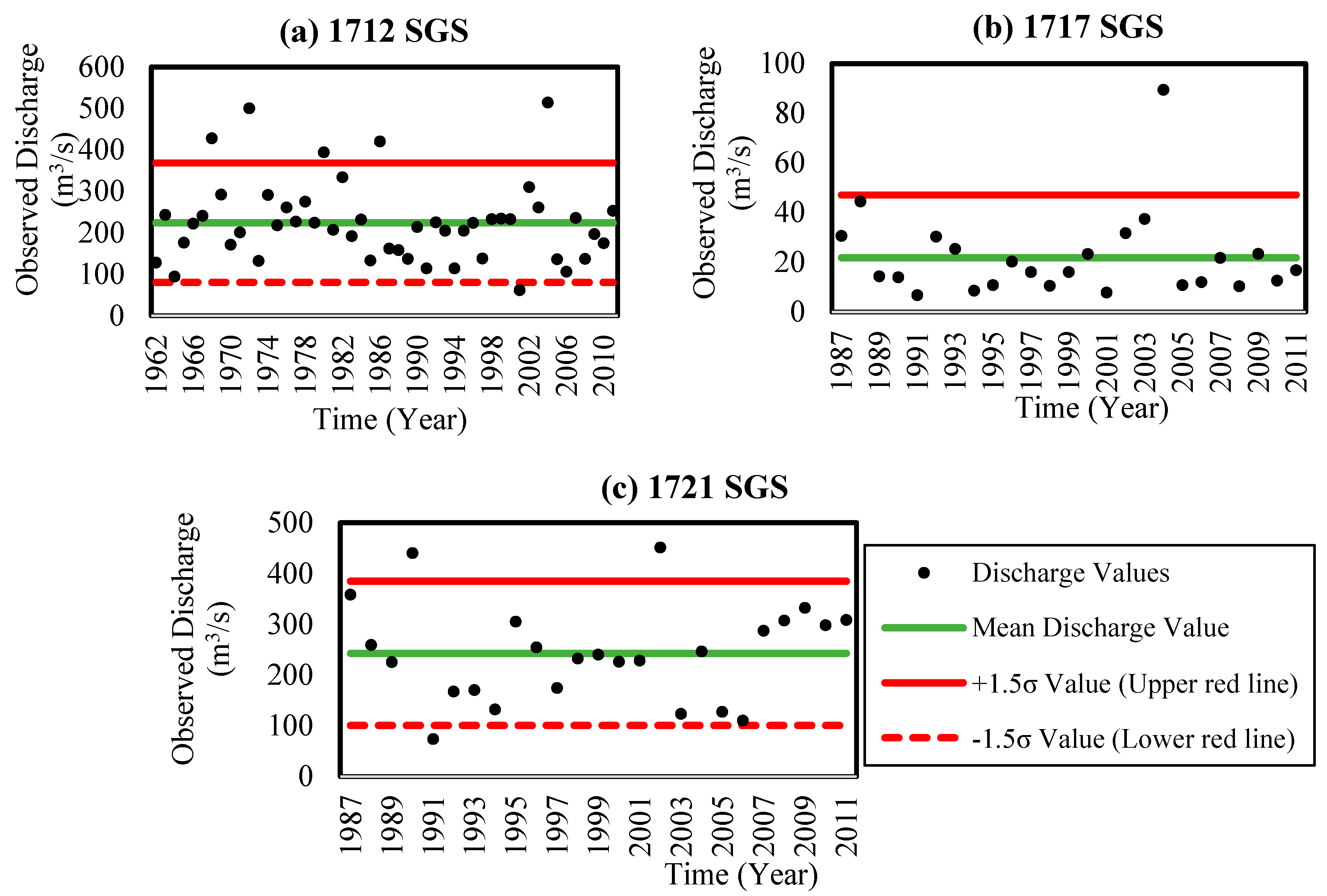
Outliers Term and Probability Distribution Functions
- n: is the number of samples;
- : is the mean value;
- : is the standard deviation.
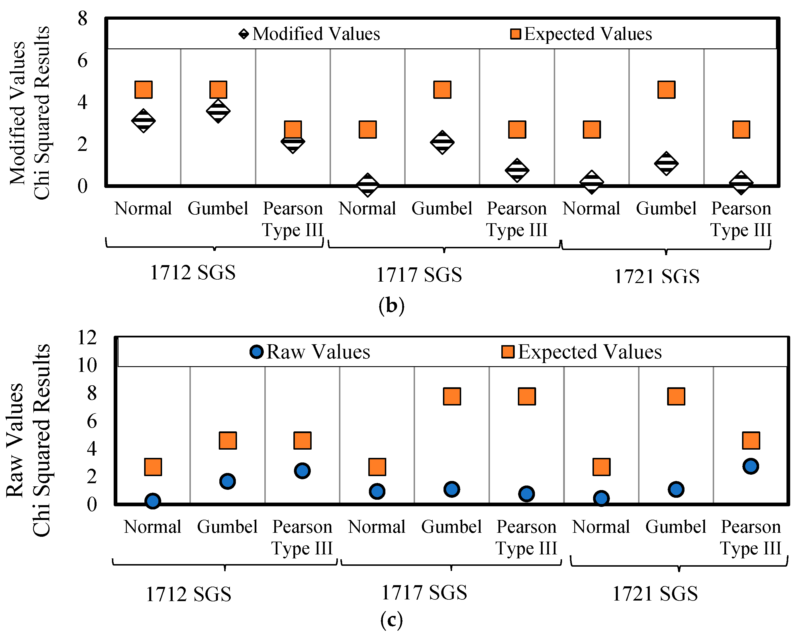
3. Results
4. Discussion
5. Conclusions
Funding
Institutional Review Board Statement
Informed Consent Statement
Data Availability Statement
Acknowledgments
Conflicts of Interest
References
- Bhat, M.S.; Alam, A.; Ahmad, B.; Kotlia, B.S.; Farooq, H.; Taloor, A.K.; Ahmad, S. Flood frequency analysis of River Jhelum in Kashmir Basin. Quat. Int. 2019, 507, 288–294. [Google Scholar] [CrossRef]
- Aghayev, A.T. Determining of different inundated land use in Salyan Plain during 2010 the Kura River flood through GIS and remote sensing tools. Int. J. Eng. Geosci. 2018, 3, 80–86. [Google Scholar] [CrossRef] [Green Version]
- Baig, M.A.; Zaman, Q.; Baig, S.A.; Qasim, M.; Khalil, U.; Khan, S.A.; Ali, S. Regression analysis of hydro-meteorological variables for climate change prediction: A case study of Chitral Basin, Hindukush region. Sci. Total Environ. 2021, 793, 148595. [Google Scholar] [CrossRef] [PubMed]
- Lotfirad, M.; Salehpoor, J.; Ashrafzadeh, A. Using the IHACRES Model to investigate the impacts of changing climate on streamflow in a semi-arid basin in North-Central Iran. Shahid Chamran Univ. Ahvaz J. Hydraul. Struct. 2019, 5, 27–41. [Google Scholar]
- Ahn, J.; Cho, W.; Kim, T.; Shin, H.; Heo, J.H. Flood frequency analysis for the annual peak flows simulated by an event-based rainfall-runoff model in an urban drainage basin. Water 2014, 6, 3841–3863. [Google Scholar] [CrossRef] [Green Version]
- Mengistu, T.D.; Feyissa, T.A.; Chung, I.M.; Chang, S.W.; Yesuf, M.B.; Alemayehu, E. Regional flood frequency analysis for sustainable water resources management of Genale–Dawa River Basin, Ethiopia. Water 2022, 14, 637. [Google Scholar] [CrossRef]
- Metzger, A.; Marra, F.; Smith, J.A.; Morin, E. Flood frequency estimation and uncertainty in arid/semi-arid regions. J. Hydrol. 2020, 590, 125254. [Google Scholar] [CrossRef]
- Sahoo, A.; Ghose, D.K. Flood frequency analysis for Menace Gauging Station of Mahanadi River, India. J. Inst. Eng. Ser. A 2021, 102, 737–748. [Google Scholar] [CrossRef]
- Ahmad, U.N.; Shabri, A.; Zakaria, Z.A. Flood frequency analysis of annual maximum streamflows using L-Moments and TL-Moments approach. Appl. Math. Sci. 2011, 5, 243–253. [Google Scholar]
- Farooq, M.; Shafique, M.; Khattak, M.S. Flood frequency analysis of River Swat using Log Pearson Type 3, Generalized Extreme Value, Normal, and Gumbel Max distribution methods. Arab. J. Geosci. 2018, 11, 216. [Google Scholar] [CrossRef]
- Guru, N.; Jha, R. Flood frequency analysis of Tel Basin of Mahanadi river system, India using annual maximum and POT flood data. Aquat. Procedia 2015, 4, 427–434. [Google Scholar] [CrossRef]
- Pekarova, P.; Halmova, D.; Mitkova, V.B.; Miklanek, P.; Pekar, J.; Skoda, P. Historic flood marks and flood frequency analysis of the Danube River at Bratislava, Slovakia. J. Hydrol. Hydromech. 2013, 61, 326–333. [Google Scholar] [CrossRef]
- Tegegne, G.; Melesse, A.M.; Asfaw, D.H.; Worqlul, A.W. Flood Frequency Analyses over Different Basin Scales in the Blue Nile River Basin, Ethiopia. Hydrology 2020, 7, 44. [Google Scholar] [CrossRef]
- Ahuchaogu, U.E.; Ojinnaka, O.C.; Njoku, R.N.; Baywood, C.N. Flood frequency analysis for River Niger at Lojoka, Kogi State using Log-Pearson Type III distribution. Int. J. Water Resour. Environ. Eng. 2021, 13, 30–36. [Google Scholar] [CrossRef]
- Turhan, E.; Değerli, S.; Duyan Çulha, B. Comparison of Different Probability Distributions for Estimating Flood Discharges for Various Recurrence Intervals: The Case of Ceyhan River. Black Sea J. Sci. 2021, 11, 731–742. [Google Scholar] [CrossRef]
- Ismail, A.Z.; Yusop, Z.; Tusof, Z. Comparison of flood distribution models for Johor River Basin. J. Teknol. 2015, 74, 123–128. [Google Scholar] [CrossRef] [Green Version]
- Majeed, A.R.; Nile, B.K.; Al-Baidhani, J.H. Selection of suitable pdf model and build of idf curves for rainfall in Najaf City, Iraq. J. Phys. Conf. Ser. 2021, 1973, 012184. [Google Scholar] [CrossRef]
- Sarfaraz, Q.; Masood, M.; Shakir, A.S.; Sarwar, M.K.; Khan, N.M.; Azhar, A.H. Flood Frequency Analysis Of River Swat Using Easyfit Model & Statistical Approach. Pak. J. Eng. Appl. Sci. 2021, 29, 8–21. [Google Scholar]
- Aydin, M. Investigation of the effect of outliers in hydrological data on flood frequency analysis. Yuz. Yil Univ. J. Inst. Nat. Appl. Sci. 2015, 20, 47–55. [Google Scholar]
- Lamontagne, J.R.; Stedinger, J.R.; Yu, X.; Whealton, C.A.; Xu, Z. Robust flood frequency analysis: Performance of EMA with Multiple Grubbs-Beck Outlier Tests. Water Resour. Res. 2016, 52, 3068–3084. [Google Scholar] [CrossRef] [Green Version]
- Saeed, S.F.; Mustafa, A.S.; Al Aukidy, M. Assessment of flood frequency using maximum flow records for the Euphrates River, Iraq. IOP Conf. Ser. Mater. Sci. Eng. 2021, 1076, 012111. [Google Scholar] [CrossRef]
- Wu, Y.B.; Xue, L.Q.; Liu, Y.H. Local and Regional Flood Frequency Analysis based on Hierarchical Bayesian model in Dongting Lake Basin, China. Water Sci. Eng. 2019, 12, 253–262. [Google Scholar] [CrossRef]
- Hlavcova, K.; Kohnova, S.; Borga, M.; Horvat, O.; St’astny, P.; Pekarova, P.; Majercakova, O.; Danacova, Z. Post-event analysis and flash flood hydrology in Slovakia. J. Hydrol. Hydromech. 2016, 64, 304–315. [Google Scholar] [CrossRef] [Green Version]
- Besha, K.Z.; Demissie, T.A.; Feyessa, F.F. Spatiotemporal trends and detection of changes in hydrological and climatic variables of Modjo River Watershed, Ethiopia. Theor. Appl. Climatol. 2021; preprints. [Google Scholar] [CrossRef]
- Chebana, F.; Dabo-Niang, S.; Ouarda, T.B.M.J. Exploratory functional flood frequency analysis and outlier detection. Water Resour. Res. 2012, 48, 1–20. [Google Scholar] [CrossRef] [Green Version]
- Heidarpour, B.; Panjalizadeh, M.B.; Ekramirad, A.; Hosseinzhad, A.; Ghasemian, L.A. Detection of outlier in flood observations: A case study of Tamer Watershed. Res. J. Recent Stud. 2015, 4, 150–153. [Google Scholar]
- Ng, W.W.; Panu, U.S.; Lennox, W.C. Chaos based analytical techniques for daily extreme hydrological observations. J. Hydrol. 2007, 342, 17–41. [Google Scholar] [CrossRef]
- Okafor, G.C.; Jimoh, O.D.; Larbi, K.I. Detecting changes in hydro-climatic variables during the last four decades (1975–2014) on Downstream Kaduna River Catchment, Nigeria. Atmos. Clim. Sci. 2017, 07, 161–175. [Google Scholar] [CrossRef] [Green Version]
- Koçyiğit, M.B.; Akay, H.; Babaiban, E. Evaluation of morphometric analysis of flash flood potential of Eastern Mediterranean Basin using principle component analysis. J. Fac. Eng. Archit. Gazi Univ. 2021, 36, 1669–1685. [Google Scholar] [CrossRef]
- Eastern Mediterranean Basin Flood Action Plan, Turkish Republic Ministry of Agriculture and Forestry. 2019. Available online: https://L24.İm/5GOD (accessed on 11 February 2022).
- Electrical Works Survey Administration-EIEI. Streamflow Observation Annuals between 1962 and 2011. Ankara, Turkey. Available online: https://www.dsi.gov.tr/ (accessed on 15 February 2022).
- Özdemir, H. Applied Flood Hydrology; The General Directorate of State Hydraulic Works (DSI): Ankara, Türkiye, 1977.
- Buldur, A.D.; Pınar, A.; Başaran, A. Göksu River flood dated 05-07 March 2004 and its effect on Silifke. J. Selcuk Univ. Soc. Sci. Institue 2007, 17, 139–160. [Google Scholar]
- Babaiban, E. Assessment of Potential Flash Flood Risk Using Morphometric Parameters: The Eastern Mediterranean Basin Case Study; Gazi Unıversity Graduate School of Natural and Applied Sciences: Ankara, Turkey, 2020. [Google Scholar]
- Oğuz, K.; Akın, B.S. Evaluation of temperature, precipitation, aerosol variation in Eastern Mediterranean Basin. J. Eng. Sci. Des. 2019, 7, 244–253. [Google Scholar] [CrossRef] [Green Version]
- Heidarpour, B.; Saghafian, B.; Yazdi, J.; Azamathulla, H.M. Effect of extraordinary large floods on at-site flood frequency. Water Resour. Manag. 2017, 31, 4187–4205. [Google Scholar] [CrossRef]
- Alberta Transportation. Civil Projects Branch. Guidelines on Flood Frequency Analysis; Alberta Transportation: Edmonton, AB, Canada, 2001. [Google Scholar]
- Grubbs, F.E.; Beck, G. Extension of sample sizes and percentage points for significance tests of outlying observations. Technometrics 1972, 14, 847–854. [Google Scholar] [CrossRef]
- Pawar, U.; Hire, P. Flood frequency analysis of the Mahi Basin by using Log Pearson Type III probability distribution. Hydrospatial Anal. 2019, 2, 102–112. [Google Scholar] [CrossRef] [Green Version]
- Buishand, T.A.; Brandsma, T. Comparison of circulation classification schemes for predicting temperature and precipitation in The Netherlands. Int. J. Clim. 1997, 17, 875–889. [Google Scholar] [CrossRef]
- Orke, Y.A.; Li, M.-H. Hydroclimatic Variability in the Bilate Watershed, Ethiopia. Climate 2021, 9, 98. [Google Scholar] [CrossRef]
- Yang, R.; Xing, B. Spatio-Temporal Variability in Hydroclimate over the Upper Yangtze River Basin, China. Atmosphere 2022, 13, 317. [Google Scholar] [CrossRef]
- Arrieta-Pastrana, A.; Saba, M.; Alcázar, A.P. Analysis of Climate Variability in a Time Series of Precipitation and Temperature Data: A Case Study in Cartagena de Indias, Colombia. Water 2022, 14, 1378. [Google Scholar] [CrossRef]
- Onen, F.; Bagatur, T. Prediction of flood frequency factor for Gumbel distribution using regression and GEP Model. Arab. J. Sci. Eng. 2017, 42, 3895–3906. [Google Scholar] [CrossRef]
- Brodie, I. Regional analysis of PROQ transforms for flood frequency estimation based on GRADEX principles. Australas. J. Water Resour. 2020, 24, 183–198. [Google Scholar] [CrossRef]
- Cong, S.; Xu, Y. The effect of discharge measurement error in flood frequency analysis. J. Hydrol. 1987, 96, 237–254. [Google Scholar] [CrossRef]
- Lalitha, S.; Tripathi, P. Detection of a pair of outliers in a sample from a Gumbel distribution with known scale parameter. J. Appl. Stat. 2018, 45, 243–254. [Google Scholar] [CrossRef]
- Amin, M.T.; Rizwan, M.; Alazba, A.A. A best-fit probability distribution for the estimation of rainfall in Northern Regions of Pakistan. Open Life Sci. J. 2016, 11, 432–440. [Google Scholar] [CrossRef]
- Feyissa, T.A.; Tukura, N.G. Evaluation of the best-fit probability of distribution and return periods of river discharge peaks. Case study: Awetu River, Jimma, Ethiopia. J. Sediment. Environ. 2019, 4, 360–368. [Google Scholar] [CrossRef] [Green Version]
- Langat, P.K.; Kumar, L.; Koech, R. Identification of the most suitable probability distribution models for maximum, minimum, and mean streamflow. Water 2019, 11, 734. [Google Scholar] [CrossRef] [Green Version]
- Mujiburrehman, K. Frequency analysis of flood flow at Garudeshwar Station in Narmada River, Gujarat, India. Univers. J. Environ. Res. Technol. 2013, 3, 677–684. [Google Scholar]
- Cerneaga, C.; Maftei, C. Flood frequency analysis of Casimcea River. IOP Conf. Ser. Mater. Sci. Eng. 2021, 1138, 012014. [Google Scholar] [CrossRef]
- Malik, M.A.; Bhatti, A.Z. Characterizing snowmelt regime of the River Swat—A case study. Tech. J. Univ. Eng. Technol. Taxila 2015, 20, 95–103. [Google Scholar]
- Bogdanowicz, E.; Kochanek, K.; Strupczewski, W. The weighted function method: A handy tool for flood frequency analysis or just a curiosity. J. Hydrol. 2018, 559, 209–221. [Google Scholar] [CrossRef]


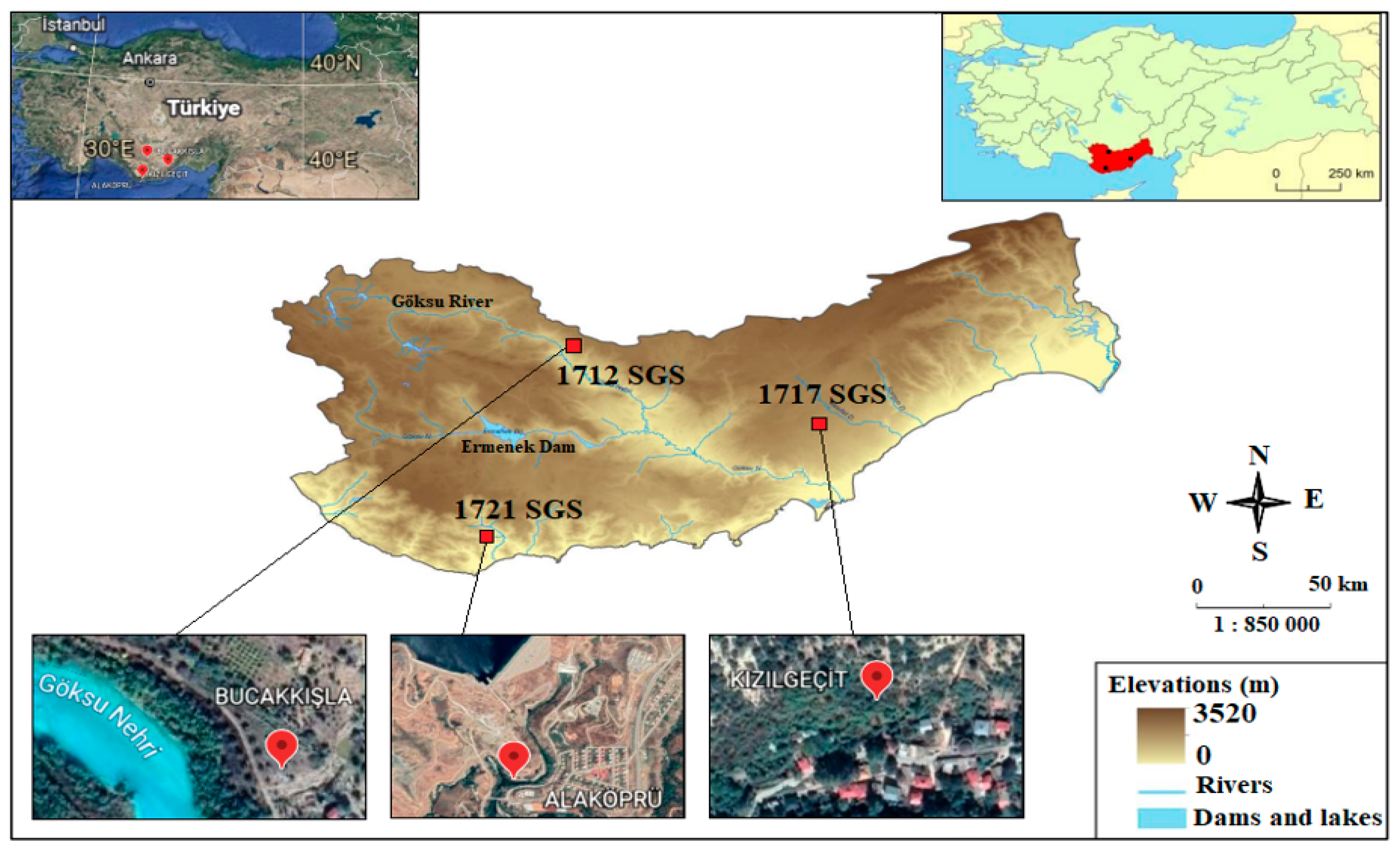
| Station | Station No | Stream | Observed Period (Year) | Average Rainfall (mm) | Elevation (m) | Average Temperature (°C) | Drainage Area (km²) |
|---|---|---|---|---|---|---|---|
| Bucakkışla | 1712 | Göksu River | 50 | 38.6 | 393 | 18.2 | 2702 |
| Kızılgeçit | 1717 | Lamas Creek | 25 | 44.4 | 975 | 12.7 | 1005.2 |
| Alaköprü | 1721 | Anamur Creek | 25 | 96.3 | 37 | 19.1 | 313.2 |
| Distribution | Constrains | Estimation Techniques | Probability Function fx(x) | Frequency Factor (Kt) |
|---|---|---|---|---|
| Normal | Scale (σ) Location (μ) | Method of Moments | Standard normal deviate z with exceedance probability 1/T | |
| Gumbel (GEV Type II) | Shape (k) Scale (σ) Location (μ) | Method of L-moments | fx(x) = | Kt = Kt = frequency factor = T = T = return period |
| Pearson Type III | Shape (α) Scale (β) Location (γ) | Maximum likelihood | α = σ/, β=, Є= µ − σ fx(x) = x: refers discharge values γ: skewness coefficient of x µ: mean of x σ: standard deviation of x | Standard normal deviate z with exceedance probability 1/T |
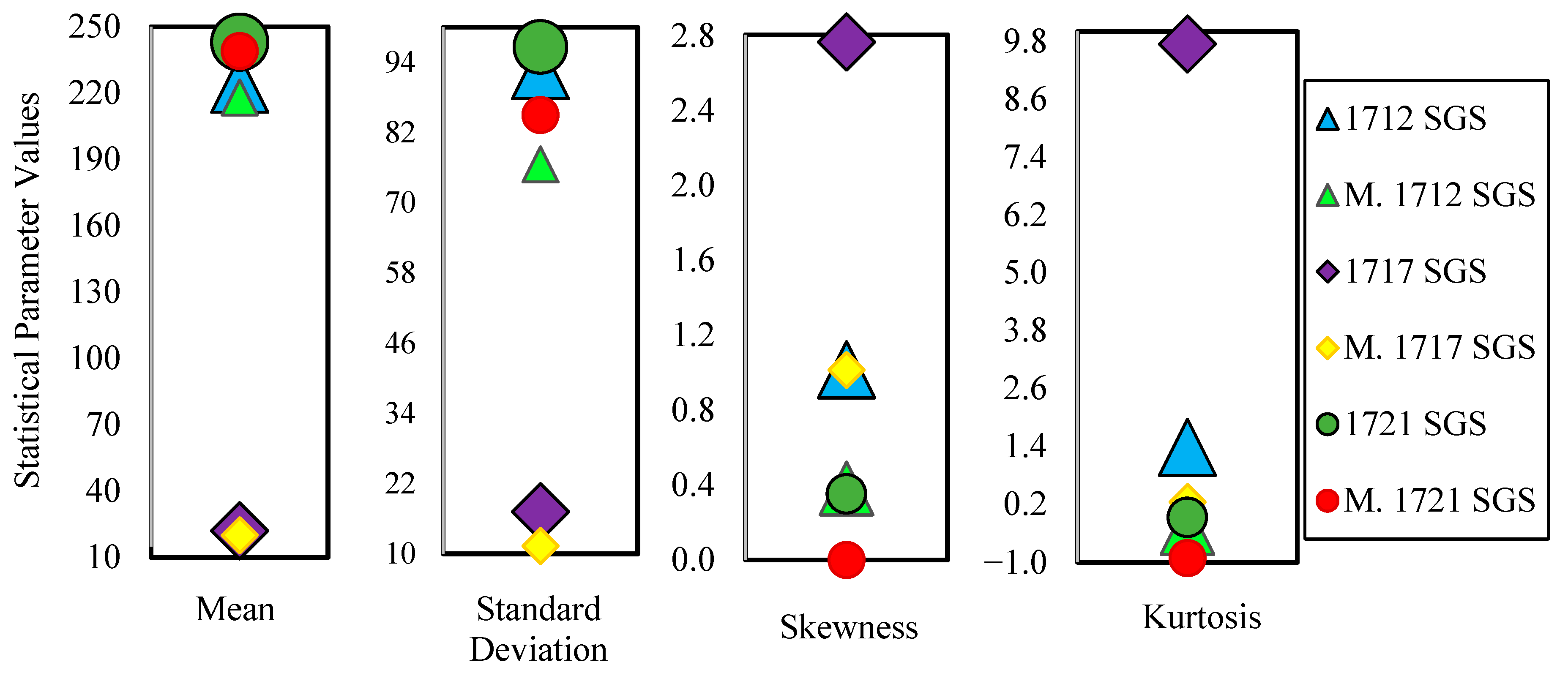
| Statistical Parameters | 1712 SGS | 1717 SGS | 1721 SGS | |||
|---|---|---|---|---|---|---|
| Value | M. Value | Value | M. Value | Value | M. Value | |
| Mean (m3/s) | 224 | 218 | 22 | 20 | 243 | 239 |
| Variance (m6/s2) | 8574 | 5862 | 295 | 129 | 9340 | 7228 |
| Standard Deviation (m3/s) | 92.60 | 76.56 | 17.19 | 11.34 | 96.64 | 85.02 |
| Skewness | 1.011 | 0.376 | 2.762 | 1.010 | 0.347 | −0.005 |
| Kurtosis | 1.381 | −0.293 | 9.742 | 0.247 | −0.075 | −0.914 |
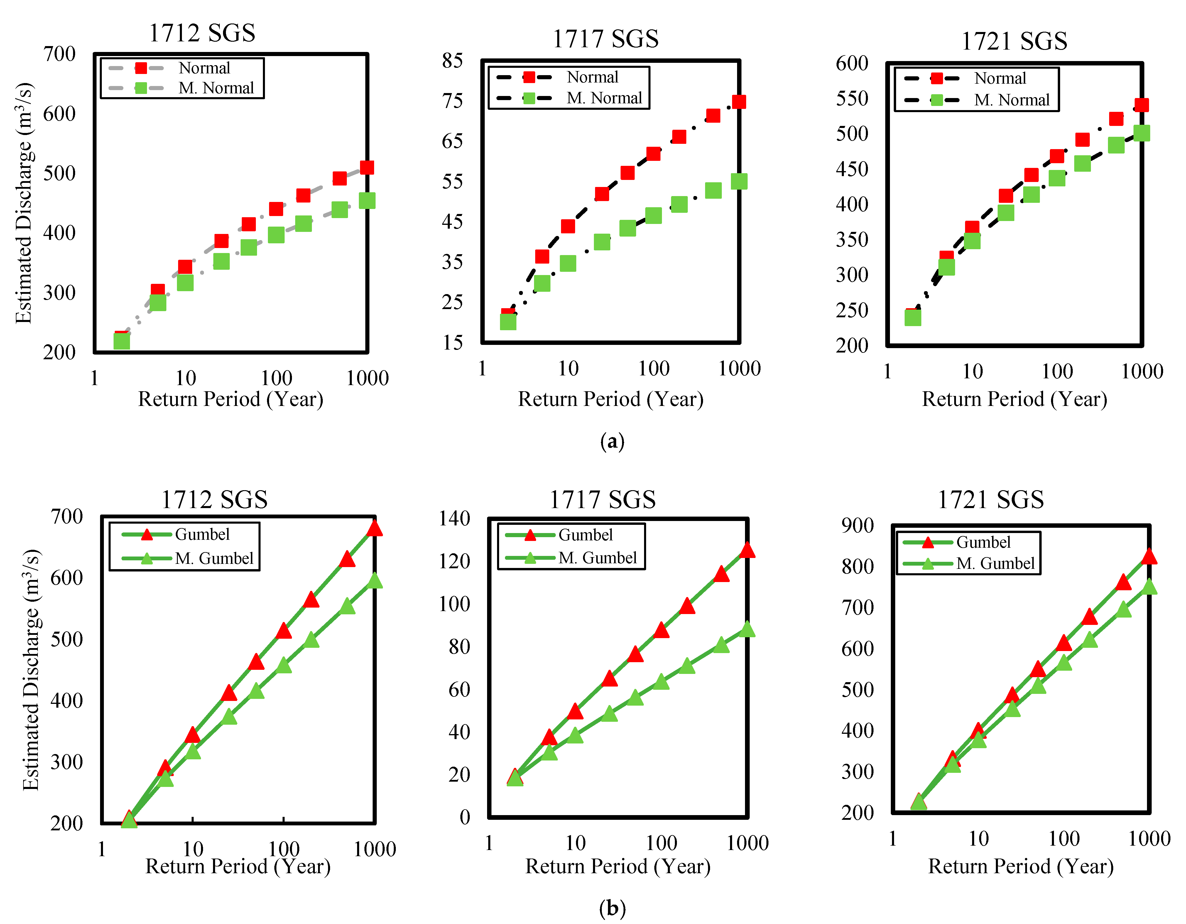
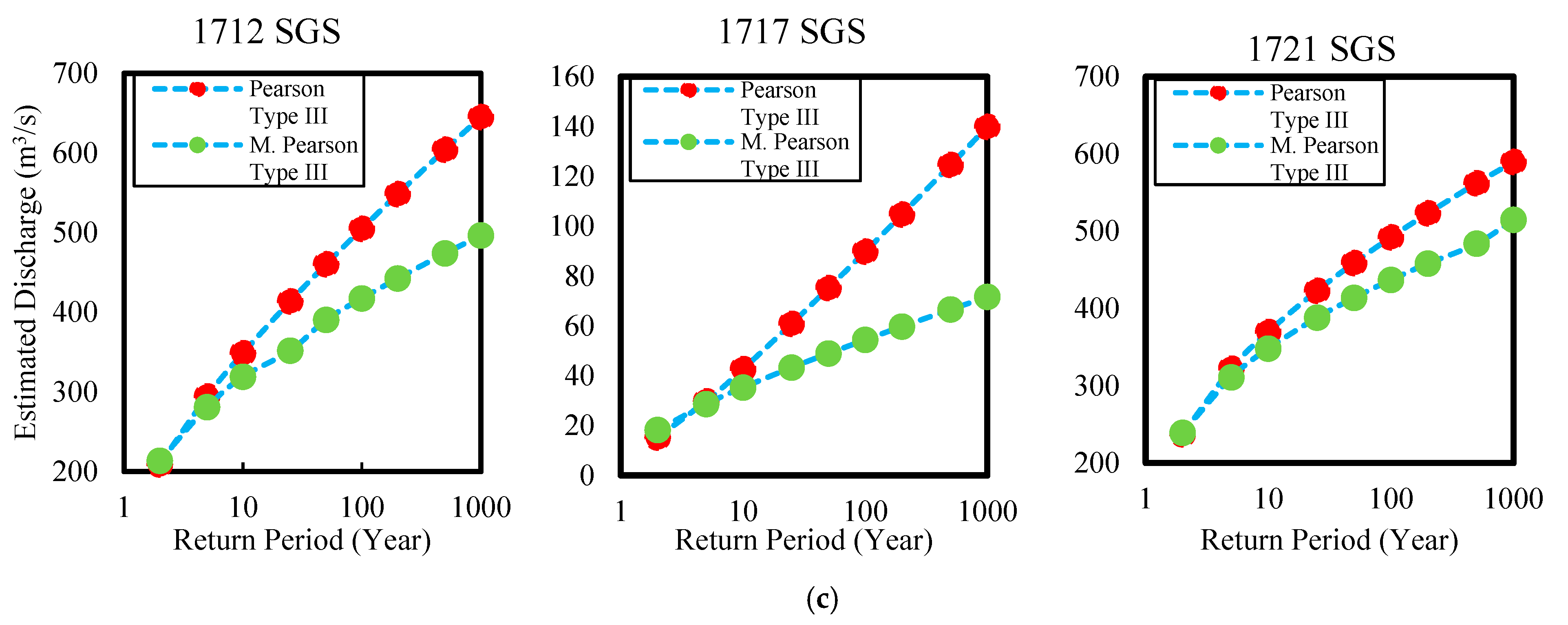
| Return Period | 1712 SGS | 1717 SGS | 1721 SGS | ||||||
|---|---|---|---|---|---|---|---|---|---|
| Normal | Gumbel | Pearson Type III | Normal | Gumbel | Pearson Type III | Normal | Gumbel | Pearson Type III | |
| 2 | 224 | 209 | 209 | 22 | 19 | 15 | 243 | 229 | 237 |
| 5 | 303 | 291 | 295 | 36 | 38 | 30 | 325 | 333 | 322 |
| 10 | 343 | 345 | 349 | 44 | 50 | 43 | 367 | 401 | 370 |
| 25 | 387 | 414 | 414 | 52 | 65 | 61 | 412 | 488 | 423 |
| 50 | 415 | 465 | 460 | 57 | 77 | 75 | 442 | 552 | 459 |
| 100 | 440 | 515 | 505 | 62 | 88 | 90 | 468 | 616 | 492 |
| 200 | 463 | 565 | 548 | 66 | 99 | 105 | 492 | 679 | 523 |
| 500 | 491 | 631 | 604 | 71 | 114 | 125 | 521 | 763 | 562 |
| 1000 | 510 | 682 | 645 | 75 | 126 | 140 | 541 | 826 | 590 |
| Return Period | 1712 SGS | 1717 SGS | 1721 SGS | ||||||
|---|---|---|---|---|---|---|---|---|---|
| Normal | Gumbel | Pearson Type III | Normal | Gumbel | Pearson Type III | Normal | Gumbel | Pearson Type III | |
| 2 | 218 | 206 | 214 | 20 | 19 | 18 | 239 | 227 | 239 |
| 5 | 283 | 274 | 281 | 30 | 31 | 29 | 311 | 318 | 311 |
| 10 | 317 | 318 | 319 | 35 | 39 | 35 | 348 | 378 | 348 |
| 25 | 352 | 375 | 352 | 40 | 49 | 43 | 388 | 455 | 388 |
| 50 | 376 | 417 | 391 | 43 | 56 | 49 | 414 | 511 | 414 |
| 100 | 397 | 459 | 417 | 47 | 64 | 54 | 437 | 567 | 437 |
| 200 | 416 | 500 | 442 | 49 | 71 | 60 | 458 | 623 | 458 |
| 500 | 439 | 555 | 474 | 53 | 81 | 67 | 484 | 697 | 484 |
| 1000 | 454 | 596 | 496 | 55 | 89 | 72 | 501 | 752 | 515 |
Publisher’s Note: MDPI stays neutral with regard to jurisdictional claims in published maps and institutional affiliations. |
© 2022 by the author. Licensee MDPI, Basel, Switzerland. This article is an open access article distributed under the terms and conditions of the Creative Commons Attribution (CC BY) license (https://creativecommons.org/licenses/by/4.0/).
Share and Cite
Turhan, E. An Investigation on the Effect of Outliers for Flood Frequency Analysis: The Case of the Eastern Mediterranean Basin, Turkey. Sustainability 2022, 14, 16558. https://doi.org/10.3390/su142416558
Turhan E. An Investigation on the Effect of Outliers for Flood Frequency Analysis: The Case of the Eastern Mediterranean Basin, Turkey. Sustainability. 2022; 14(24):16558. https://doi.org/10.3390/su142416558
Chicago/Turabian StyleTurhan, Evren. 2022. "An Investigation on the Effect of Outliers for Flood Frequency Analysis: The Case of the Eastern Mediterranean Basin, Turkey" Sustainability 14, no. 24: 16558. https://doi.org/10.3390/su142416558
APA StyleTurhan, E. (2022). An Investigation on the Effect of Outliers for Flood Frequency Analysis: The Case of the Eastern Mediterranean Basin, Turkey. Sustainability, 14(24), 16558. https://doi.org/10.3390/su142416558