Article

Assessment of Outdoor Design Conditions on the Energy Performance of Cooling Systems in Future Climate Scenarios—A Case Study over Three Cities of Texas, Unites States

1
Instituto Universitario de Arquitectura y Ciencias de la Construcción, Escuela Técnica Superior de Arquitectura, Universidad de Sevilla, 41012 Sevilla, Spain
2
Department of Landscape and Architecture, Texas A&M University, College Station, TX 77843, USA
3
Department of Architecture, Faculty of Art, Tarbiat Modares University, Tehran 13145-1696, Iran
4
Department of Building Installations, Building and Housing Research Center (BHRC), Tehran 13145-1696, Iran
5
Department of Earth Sciences, Indian Institute of Technology Roorkee, Roorkee 247667, Uttarakhand, India
*
Author to whom correspondence should be addressed.
Sustainability 2022, 14(22), 14848; https://doi.org/10.3390/su142214848
Submission received: 13 October 2022 / Revised: 28 October 2022 / Accepted: 7 November 2022 / Published: 10 November 2022

Abstract

:
The excessive use of energy in buildings due to increased populations and economic development leads to more greenhouse gas emissions, which affect climate change and global warming. Changes in prevailing outdoor weather conditions significantly affect the energy systems of buildings through increased cooling and decreased heating. In this paper, 30 years of data of dry and wet bulb temperatures (1990–2020) with a time interval of 3 h were considered in order to estimate the climatic outdoor design conditions in the cities of Dallas–Fort Worth, Houston, and San Antonio in the state of Texas. The results suggest that the dry bulb temperature (DBT) had significantly higher increases in Dallas–Fort Worth (2.37 °C) than the wet bulb temperature (WBT) in Houston (4.1 °C) during the study period. Furthermore, this study analyzed the effects of climate change on cooling degree hours (CDH) and heating degree hours (HDH) and the results suggest the most significant drop in HDH in Dallas–Fort Worth with a maximum CDH fluctuation as compared to other two cities. The effect of climate change on the performance of cooling systems is also investigated in this study via direct evaporative coolers (DECs) and direct-indirect evaporative coolers (IDEC), which do not perform well in the selected cities. In contrast, absorption system (Abs) and vapor compression (VC) systems show an increase in the number of additional loads. The second part of this study is related to the future projection using the ARIMA model, which suggests that DBT would rise significantly in Houston (from 37.18 °C to 37.56 °C) and Dallas–Fort Worth (39.1 °C to 39.57 °C) while diminishing in San Antonio (from 34.81 °C to 33.95 °C) from 2020 to 2030. In contrast, WBT will experience an upward trend in Houston (from 36.06 °C to 37.71 °C) and Dallas–Fort Worth (from 31.32 °C to 31.38 °C) and a downward trend in San Antonio (from 32.43 °C to 31.97 °C) during 2020–2030. Additionally, the future performance prediction of Abs and VC systems is also performed, which reveals that the amount of additional load required is significantly higher in 2030 compared to 2020 and is more prominent in Houston. Conversely, amount of additional load required for cooling systems in San Antonio shows a decreasing trend in 2030.

1. Introduction

Due to global warming and shifts in demographic populations from rural areas to cities, the amount of energy consumed by buildings has been significantly affected by climate change [1,2] and has exerted adverse effects on the peaking time and emission peaks of building energy use and carbon emissions [3,4,5,6]. According to dynamic simulation research by Huo et al. (2021), urban carbon emissions will continue to climb and reach their peak in 2040 if the necessary policies are not applied [7]. It is estimated more than half of the world’s population will live in megacities and will produce more than 70% of energy and CO2 [8]. In this regard, urban sustainability has emerged as a defining challenge in the 21st Century. In U.S. cities with increasing populations, the building sector represents a large share of the final energy demand [9]. The electricity use for building space cooling by the residential and commercial sectors was ∼10% of total U.S. electricity consumption in 2019 [10]. In addition, because of climate change, building energy consumption for cooling has been increasing and the demand for cooling energy is projected to continue to grow in the coming decades [11,12,13]. Many regions have set ambitious sustainability targets to reduce emissions and energy consumption. For example, New York has set a target of reducing total emissions by 45% from 1990 levels by 2030 and the California government has established the Clean Energy and Pollution Reduction Act, which aims to reduce green gas emissions by 40% from 1990 levels by 2050 [3,14]. Thus, forecasting urban building energy consumption accurately is critical to accelerating the transition to sustainable cities [15].
Climate change considerably affects the behavior of the dry bulb temperature (DBT) and wet-bulb temperature (WBT). The DBT impacts the number of heat losses, increasing through the building envelope, and the subsequent electricity use for the corresponding logical cooling and heating needs. The WBT dominates the quantity of dehumidification required on dry winter days and the latent heat portion of cooling energy in humid summer conditions [16,17]. In recent years, climate change has not only led to an increase in the DBT, but it has also influenced the moisture value of the air, which is why the greenhouse effect has also intensified, given that the increase in outdoor DBT and WBT generates latent and sensible load as the seasons’ progress, thereby increasing the building’s cooling load. Therefore, by increasing the humidity value of the outside air, more extensive heating, ventilation, and air conditioning units (HVAC) have been needed to dehumidify the air and achieve convenient conditions [18].
Several studies have evaluated the impacts of climate change on building energy consumption in the U.S. using various numerical simulations. Zhou, Eom, and Clarke (2013) predicted that U.S. building energy consumption would decrease at most by 6% in the 21st century based on the three HadCM3 Global Circulation Models (GCMs) [19]. Wang and Chen (2014) investigated the impact of climate change on various types of residential and commercial buildings in the seven climate zones through Energy Plus simulations. They reported a net rise in energy consumption by the 2080s for climate zones 1–4 (hot humid, warm humid, marine, and mixed humid) and a net reduction in climate zones 6–7 (cold and very cold) [20]. Zhou et al. (2014) predicted the U.S. state-level building energy demands by 2095 using the Global Change Assessment Model (GCAM) and indicated the existence of large spatial heterogeneity in climate-induced building energy ranging from −10% to +10% for a total at the state level [21]. Chakraborty’s recent study (2021) predicted persistent, incremental changes in cooling energy consumption from 2020 to 2100 using an explainable artificial intelligence (XAI) model. The maximum incremental impacts of 87.2% in hot–humid and 121% in mixed–humid climate regions are expected under scenarios of increased reliance on fossil fuels (SSP585) [22]. For the coastal regions of New York and San Francisco, increases in cooling demand of approximately 8% and 10%, respectively, were projected [23,24].
Texas’ energy consumption is significantly coupled with changes in climate and weather conditions. In 2019, Texas was the largest energy-producing but also the most energy-consuming state in the U.S. The increase in energy demand associated with weather conditions was approximately 53% of the peak and was primarily based on demands in residential areas [25]. Although energy consumption for residential and commercial buildings in Texas is projected to decrease due to energy efficiency improvements, meeting the peak load energy demand will be challenging due to the impacts of population growth and climate change. Given that U.S. energy demands have high variability and large spatial heterogeneity based on the geographic context [21], assessing climatic design conditions and the additional energy needed to operate cooling systems at the city level is a must.
Although the effects of climate change on building energy consumption have frequently been explored in various regions and scenarios, evaluation on the city scale that allows decision-makers and stakeholders to accomplish sustainable development is largely limited. Therefore, this study aims to explore how outdoor climatic design conditions have changed over the past 30 years (1990–2020) and evaluate how the operation of cooling systems and cooling and heating degree hours have changed under the influence of climate conditions. Finally, the performance of buildings’ cooling systems in Texas was evaluated based on climatic changes. Therefore, this study aims to answer the following research questions:
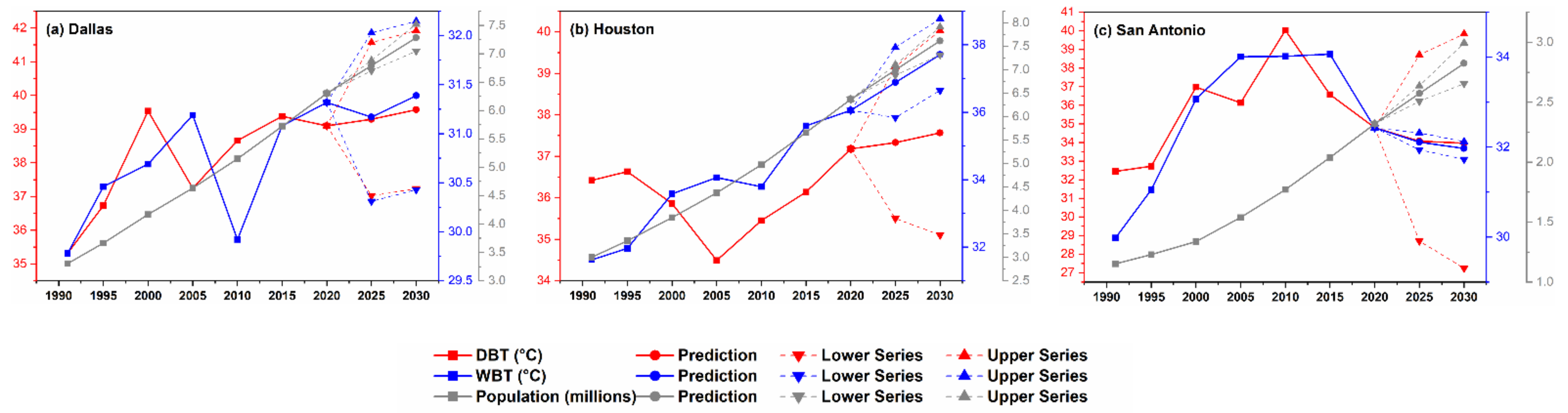
  • Q1: What is the impact of climate change on climatic outdoor design conditions based on the technical report of ASHRAE (DBT and WBT)?
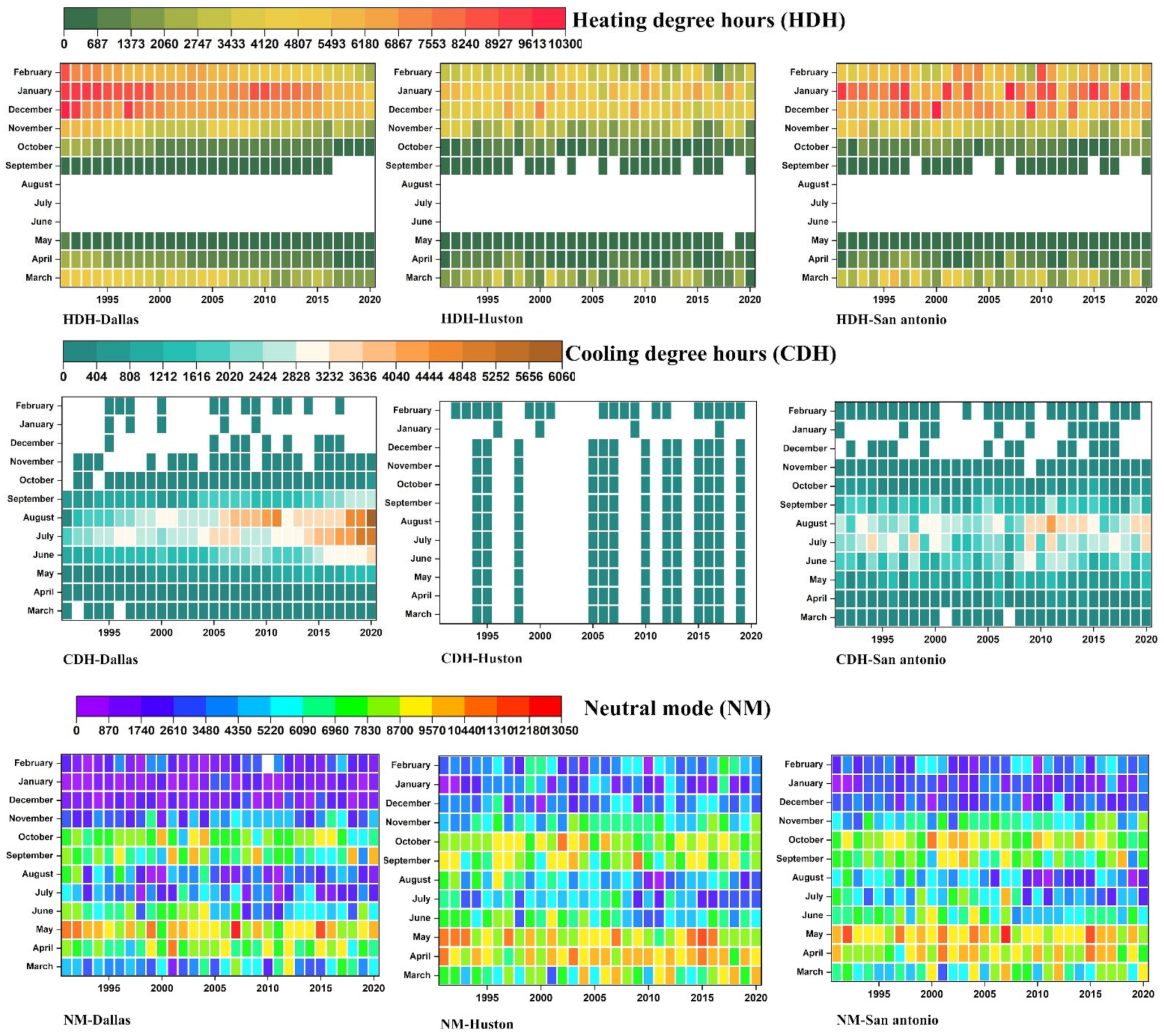
  • Q2: How has climate change impacted the process of cooling degree hours (CDH) and heating degree hours (HDH)?
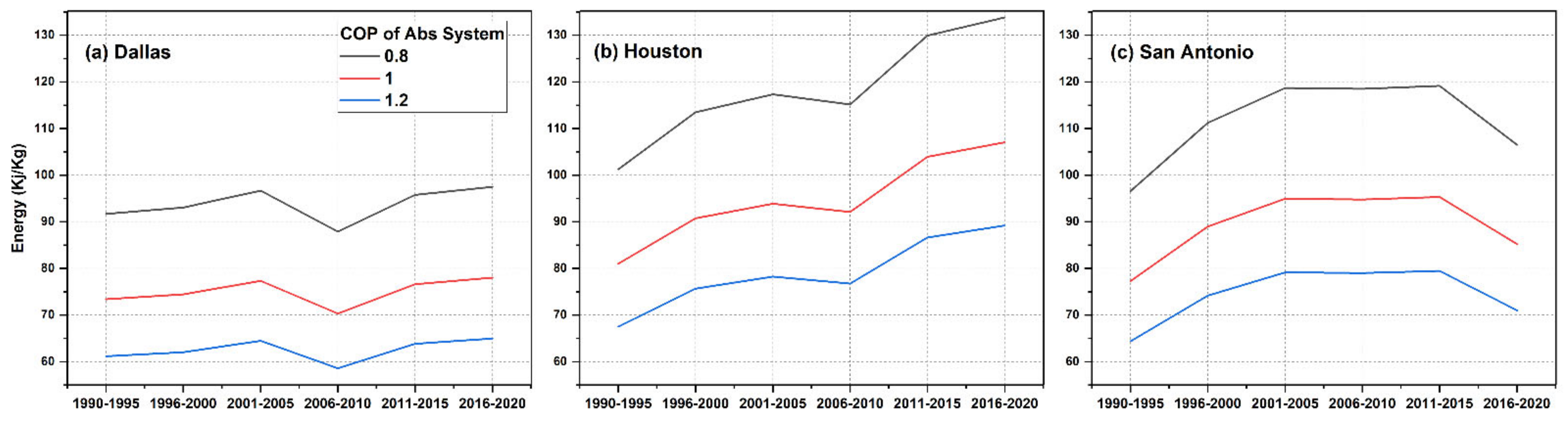
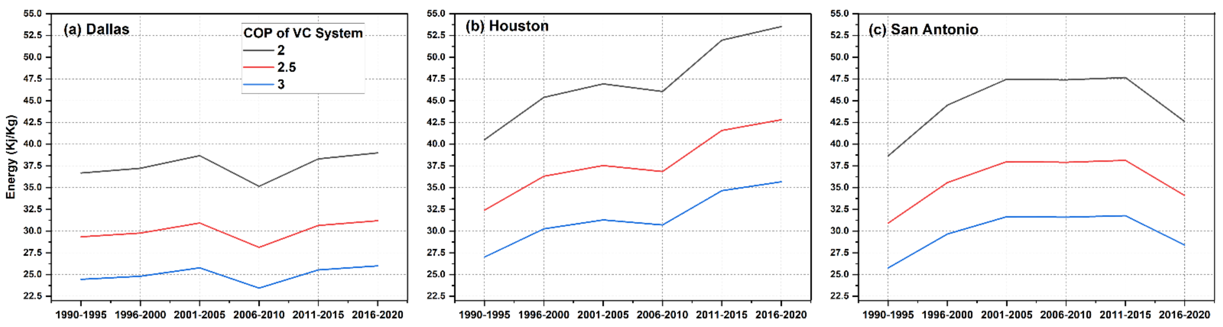
  • Q3: To what extent have climate changes impacted the operation of cooling systems, specifically on absorption (Abs) and vapor compression (VC)?
After evaluating climatic outdoor design conditions in terms of both dry bulb temperature (DBT) and wet bulb temperature (WBT), based on the ASHRAE technical report [26], the first section of the study looks at the demographic trend impact on DBT and WBT in selected cities over thirty years (in each five-year interval). In the second part, the impact of climate change on variations in cooling degree hours (CDH), heating degree hours (HDH), and neutral mode (NM) parameters are evaluated under the influence of the DBT trend. Lastly, particular attention is paid to predicting climatic change and energy demands of cooling systems for the next decade (2020–2030) based on the variations in the last 30 years (1990–2020) obtained with the auto-regressive integrated moving average (ARIMA) method.

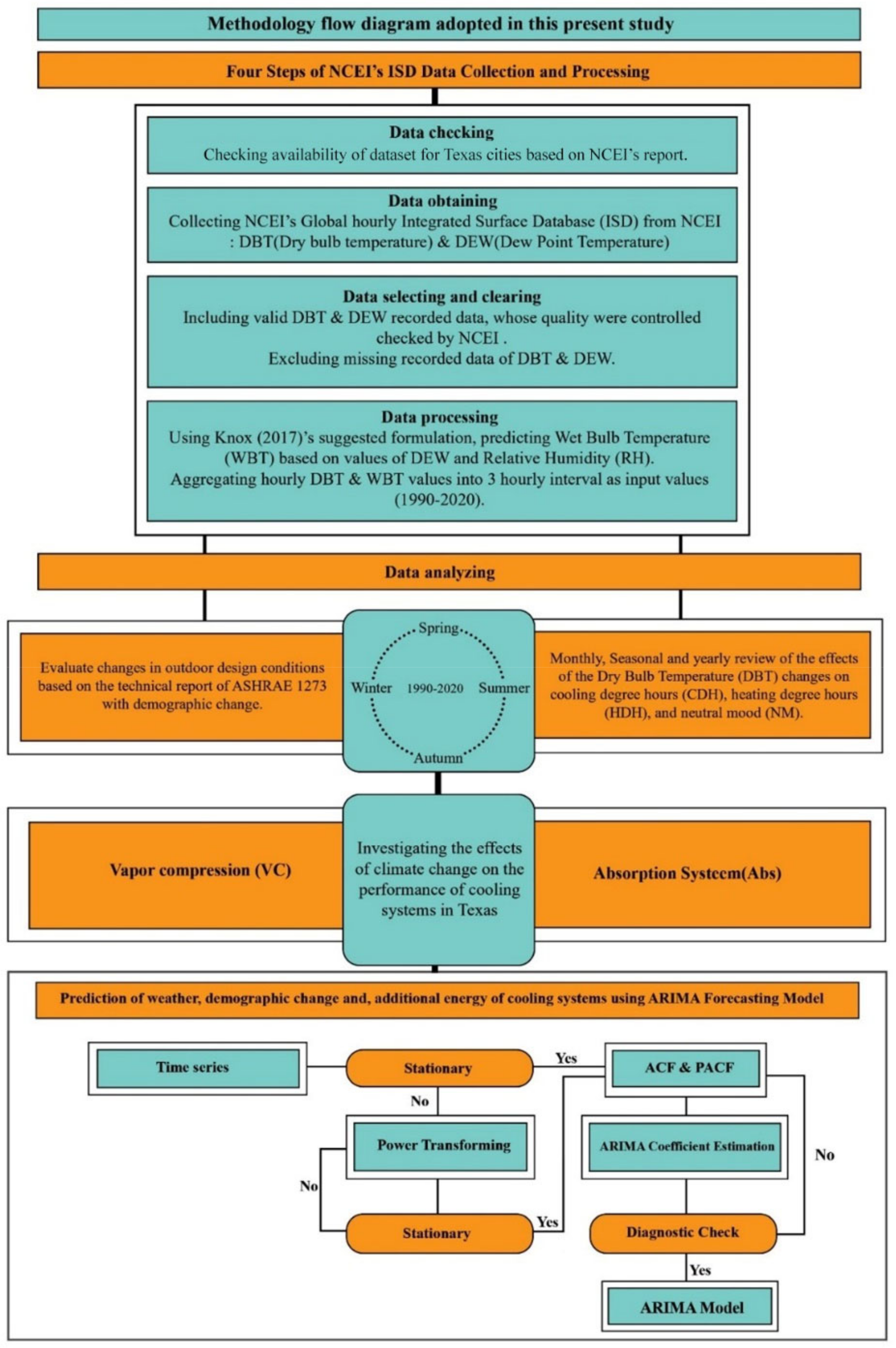
2. Materials and Methods

This study considered three major cities in Texas, namely Dallas–Fort Worth, Houston, and San Antonio, because of the unexpectedly high summer peak demands for electricity due to global warming, which have grown at a rate of about 1.6% per year [27]. In this regard, evaluating cooling energy use for future climate prediction at the subnational level will offer helpful insights into Texas’s climate policy and regional energy system planning. Figure 1 illustrates the methodological flow diagram adopted in this study.

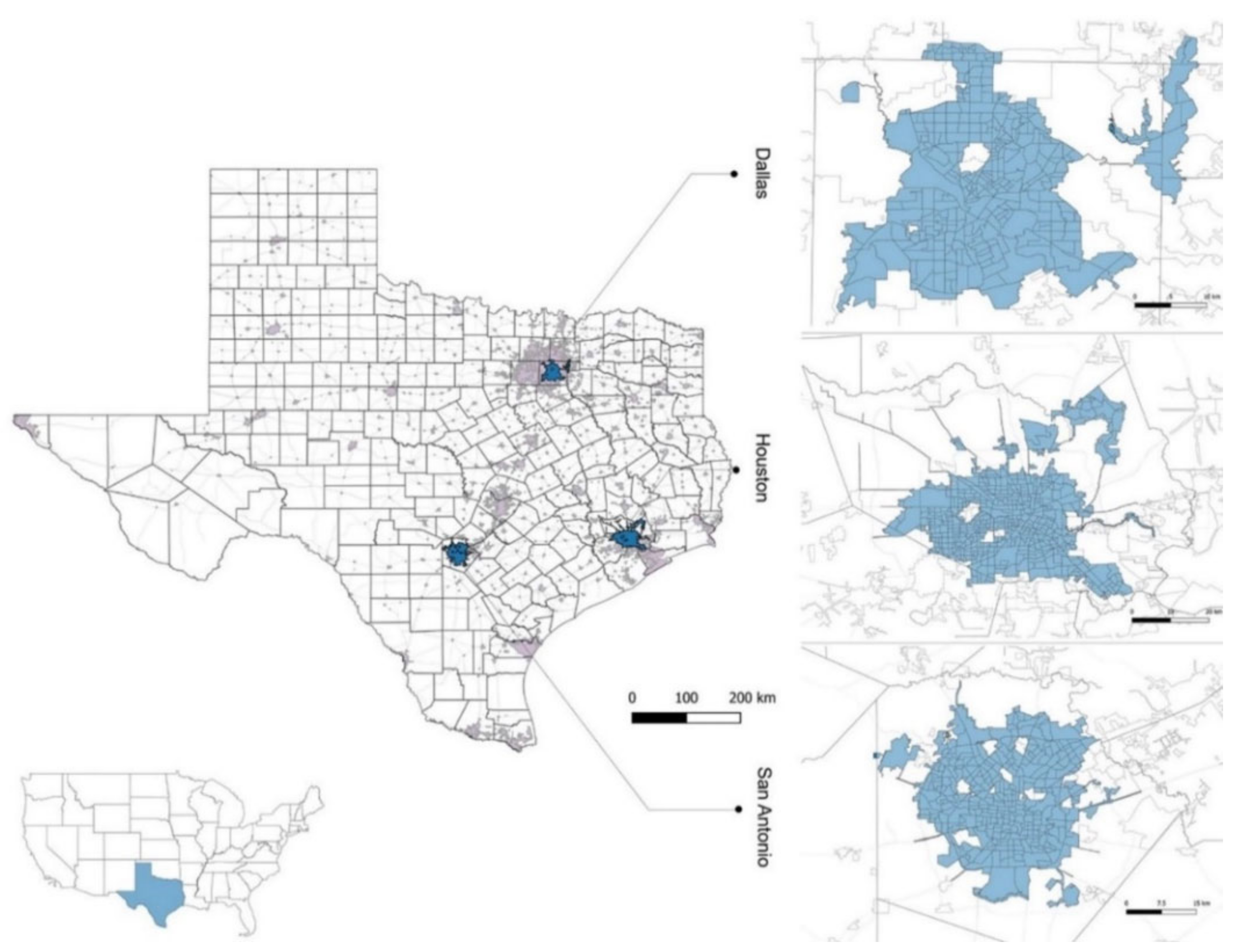
2.1. Selected Cities

2.1.1. Overview of Selected Cities in Texas

Texas is a state in the central south of the United States with an area of 695,662 sq km and more than 29.1 million residents in 2020. Three major cities, i.e., Houston, San Antonio, and Dallas–Fort Worth, form Texas’s economic, business, and cultural hubs. The region’s largest statistical area and the highest population comprised the study area. The part of Texas that lies east of Interstate 35 experiences a subtropical climate, while regions west of the Interstate are arid deserts. Houston, San Antonio, and Dallas–Fort Worth belong to a typical humid subtropical climate.
There are two significant reasons for studying these cities. First, they are the most populous cities in Texas to suffer from severe heat stress due to global warming [28,29,30]. The extreme monthly summertime temperature trends in those cities indicate an increase of about 17.22 °C compared to the 1950–1999 average, which implies increased frequencies and intensities of heatwaves and urban heat islands [31]. Considering the current population and its growth rates in the studied cities [32], predicting future summer energy demands for cooling is necessary to achieve the goal of net-zero carbon emissions by 2050. Secondly, although the three cities vary in geographical features, all these cities have a humid subtropical climate. For example, Houston is a coastal megacity along the Mexican Gulf Coast with relatively high summer precipitation. In contrast, San Antonio and Dallas–Fort Worth are located on the southern plains of Texas, a semi-arid region. Therefore, the current analysis can capture the spatial variation of predictive building energy demand generated by geographical features.

2.1.2. Climate Conditions of Selected Study Cities in Texas

Global warming and rising trends in greenhouse gas emissions are changing the climate in Texas [33] and raising expectations of various environmental impacts, including rising sea levels, more frequent extreme weather events, and increased pressure on water resources [34]. Heat is the leading climate change risk facing Texas. The average annual temperature in Texas is expected to be 16.11 °C warmer by 2036 than the average of the 1950s. The number of 100-degree days is expected to nearly double compared to 2000–2018, especially in urban areas [31]. Accordingly, the energy demand in Texas has been affected by ongoing changes in climate and weather conditions. The increase in demand associated with weather conditions is approximately 53% of the peak, based primarily on residential demand [25]. While energy consumption projections for residential and commercial buildings in Texas are expected to decrease due to improvements in energy efficiency, population growth and climate change effects are the leading causes of this incoming stress on building energy demand [10]. Due to the vast size of Texas, the cities surveyed in this study have a wide range of climatic features discussed below.

Dallas–Fort Worth

In northern Texas, Dallas–Fort Worth (Figure 2) has a total area of 990 km2, making it the largest city in the state. With a population of 1,300,000, it is the ninth most populous city in the United States and the third largest in Texas after Houston and San Antonio [32]. Dallas–Fort Worth has a humid subtropical climate (Cfa in the Köppen classification), which is characteristic of the southern plains of the United States. It also has continental features and a relatively wide annual temperature range. The summer season in Dallas–Fort Worth is very hot and humid, although low humidity characteristics of desert locations appear [35]. July and August are typically the hottest months, with an average high of 36 °C. Heat indexes often exceed 41 °C in the height of summer. Winters in Texas range from cold to mild, with occasional cold spells. January is the coldest month, with an average daytime high of 14 °C. Meanwhile, spring and fall have pleasant weather with mild temperatures.

Houston

Houston is the fourth most populous city in the United States. In Texas, it is the most populous city, with a population of 2,300,000 in 2020 [32]. With a total area of 1600 km2, the city is located in southeast Texas near Galveston Bay and the Gulf of Mexico (Figure 2). Houston has a humid subtropical climate (Cfa in the Köppen classification), which is typical of the southern United States. The city has four distinct seasons in terms of temperature but only two seasons in terms of weather, i.e., rainy (from April to October) and dry (from November to April). Throughout the year, the prevailing wind from the south and southeast delivers heat and moisture from the nearby Gulf of Mexico and Galveston Bay. As a result, Houston’s summer is very hot and humid, with frequent showers and thunderstorms, high temperatures exceeding 32 °C, and 90% relative humidity [35].
Conversely, winters in Houston are relatively temperate and dry. In January, the coldest month, the average high and low are 17.2 °C and 6.2 °C, respectively. Spring and fall are warm, however, with temperatures ranging between 20 °C and 28 °C during the daytime hours [35].

San Antonio

San Antonio is the seventh most populous city in the United States and the second most populous city in Texas, with 1,400,000 residents in 2020 [32]. With a total area of 1200 km2, the city is located in southern Texas, 200 km from the Gulf of Mexico (Figure 2). It was ranked in the top ten fastest growing cities in the United States from 2000 to 2010 (U.S. Census Bureau, 2011). San Antonio has a humid subtropical climate (Cfa in the Köppen classification), featuring typically very hot, humid, and muggy summers and mild winters [35]. July and August are summer months with an average high of 35 °C. January is the coldest winter month but is relatively warmer than most other Texas areas. The average annual precipitation is 737 mm, with a maximum of 1320 mm and a minimum of 250.0 mm in one year [35]. In particular, the three months of May, June, and October have higher average precipitation.

2.2. Climatic Data

To evaluate climatic outdoor design conditions, it is necessary to consider annual simple climate design values according to the 2005 ASHRAE Handbook-Fundamentals [26]:
  • 99.6% and 99% heating DBT;
  • 0.4%, 1%, and 2% cooling DBT;
  • 0.4%, 1%, and 2% evaporation WBT.
The x% simple design condition is the condition that is exceeded, on average, x% of the time frame under consideration. For example, the 1% annual design dry-bulb temperature is the temperature that is exceeded on average for 1% of the hours of the year. To calculate design conditions, researchers require access to long-term hourly meteorological data, the values of which are prepared by the Integrated Surface Database (ISD) (NOAA IDE), a global database that consists of hourly and synoptic surface observations. The database incorporates data updated daily from over 35,000 stations worldwide and more than 14,000 active ISD stations and has the best spatial coverage in North America, Europe, Australia, and parts of Asia. The observed input sources used in ISD are processed through automated and manual quality control (QC) that is applied to the entire ISD archive. To ensure the high validity and accuracy of the observed datasets, QC includes algorithms that aim to check for proper data format for each field, extreme values and limits, consistency between parameters, and continuity between observations [36,37]. Some design conditions were evaluated in a prior edition of the ASHRAE Handbook [38] by applying common frequency matrices. For example, the 0.4% dry-bulb design condition had been calculated by totaling rows in the (dry-bulb, dewpoint) joint frequency matrix, which resulted in indices such as DBT and dew point temperature not being considered. In the new edition [26], however, the frequency vectors were formed by the number of hours (Nbin) within each temperature interval (bin). The present study estimates the frequency vector for a total period of 30 years (from 1990 to 2020) at successive five-year interval periods (six different time frames: 1990–1995, 1995–2000, 2000–2005, 2005–2010, 2010–2015, and 2015–2020). Considering the bin method, eight daily 3 h shifts were calculated (10:30–1:30, 1:30–4:30, 4:30–7:30, 7:30–10:30, 10:30–13:30, 13:30–16:30, 16:30–19:30, and 19:30–22:30) by averaging over the years of each time period. This study utilized the cumulative sum of the frequency vectors used to determine the design conditions for a given percentage of time to estimate the distribution function.

2.3. Calculation Methods

According to ASHRAE report 1273 [26], DBTs values are grouped by equal bins (0.5 °C) and, if all DBTs are satisfying based on Equation (1), the frequency vector counts each value of F D B k .
D B T k D B T 2 D B T < D B T k + D B T 2
where ΔDBT is the interval of the bin and D B T k is the center of the bin k. The cumulative distribution function (CDF) is obtained by summing all hours below a certain level.
C F D D B k = i < k F D B i i F D B i
  C F D D B k indicates the probability (P) that the DBT is lower than the upper limit of the bin.
C F D D B k = P |   D B T < D B T k + D B T 2
Moreover, considering that sensible and latent heat load depends on the difference of DBT and humidity between indoor and outdoor environments, respectively, these values are extracted from the analysis of outdoor design conditions over a period of 30 years. After calculating these differences as monthly, their annual value has been estimated for the desired period (1990–2020) and, eventually, the trend of latent and sensible load over each five-year period is presented.
In the second part, the impact of climate change on the rate of cooling degree hours (CDH), heating degree hours (HDH), and neutral mode (NM) as influential indexes in choosing the cooling system for selected cities between 1990–2020 have been analyzed. As per ASHRAE, 2001 [39,40], if the temperature for the hour falls below the heating base temperature of 18 °C, the degree hour is recorded as a heating degree hour (Equation (4)), and if the average air temperature for the hour rises above the cooling base temperature of 26 °C, the degree of cooling is recorded (Equation (5)). The CDH and HDH index enables relatively effortless estimation of part-time operation for each month (season) and average cooling and heating load profiles for day and night-time independently, when cooling or heating is needed, and is simpler and more effective than other prediction models [41,42]. Moreover, the number of degree hours that can be lived in each city with different seasons without a heating and cooling system is called the neutral mood. This index, which is in the range between CDH and HDH values, has also been analyzed between 1990 and 2020 in the three selected cities of the state of Texas in this research.
HDH = (18-DBT) × the number of intervals hours recorded
CDH = (DBT-26) × the number of interval hours recorded
Another research goal of this study is dedicated to the influence of climate changes on the performance of cooling device systems of buildings in Dallas–Fort Worth, Houston, and San Antonio. Thermal comfort is created in the psychrometric chart when the temperature is between 22 °C and 27 °C and the relative humidity φ is between 40% and 60% [43,44]. The climatic outdoor design conditions of the studied cities have placed the DBT outside of this range (Table 1) and the direct evaporative cooler (DEC) and direct—indirect evaporative cooler (IDEC) systems do not perform well or create thermal comfort conditions. Vapor compression (VC) and absorption systems (Abs) are the essential cooling systems in creating thermal comfort conditions used in these areas [45,46]. VC systems efficiently move heat from a cold source to a hot heat sink (usually air) and the heart of the system is the compressor. Unlike such systems, which use electrical energy and compressors in the compression refrigeration cycle [47], Abs systems remove the compressor and use thermal energy to produce refrigeration, thus reducing power consumption [48,49]. As the coefficient of performance (COP) is usually used to evaluate different types of heat pump systems, the amount of energy required by each system can be assessed and compared. To calculate the COP of Abs, the amount of cooling load and the energy generator required to produce refrigerant vapor is needed, while in VC systems the work required by the compressors and other cycles as well as the amount of cooling load is needed, which is obtained using Equations (6) and (7).
C O P v c = Q c o o l W v c
C O P A b s = Q c o o l Q g e n e r a t o r

2.4. ARIMA Forecasting Model

To evaluate the future performance of the indicators, the accurate forecasting of time series is essential. Univariate time series forecasting is a flexible and easy-to-use multidisciplinary scientific tool requiring only historical observations. One such model is the ARIMA (Auto-Regressive Integrated Moving Average), initially developed by Box and Jenkin in 1976 [50]. The ARIMA performance is relatively better at predicting weather conditions in comparison with artificial neural network (ANN) models [51,52]. ARIMA techniques are considered smooth for forecasting and are more frequently used when the data series is of a long duration and the correlation between the past observations is stable [53]. The ARIMA model considers the general equation of successive differences at the dth difference of X t as follows using Equation (8):
d X t = 1 B d X t
where d is the different order and B is the backshift operator.
The successive difference at a one-time lag is calculated using Equation (9).
1 X t = 1 B X t = X t X t 1
The ARIMA (p, d, q) is generally expressed as shown in Equation (10) [54]:
Φ p B W t = θ q B e t
where Φ p B is the autoregressive operator of p order, θ q B is the moving average operator of q order, and W t = d X t .
In this study, we have used the auto-ARIMA function (pmdarima) in Python to determine the best (p, d, q) value based on the autocorrelation function (ACF) and partial autocorrelation function (PACF) diagram. The ACF and PACF diagrams and standardized residual plot were used to determine the model’s reliability, accuracy, suitability, and performance. In addition to the standardized error, RMSE is also calculated between the actual ( X o ) and forecasted ( X t ) observations, as shown in Equation (11).
  R M S E = i = 1 n X t X o 2 n

3. Results and Discussion

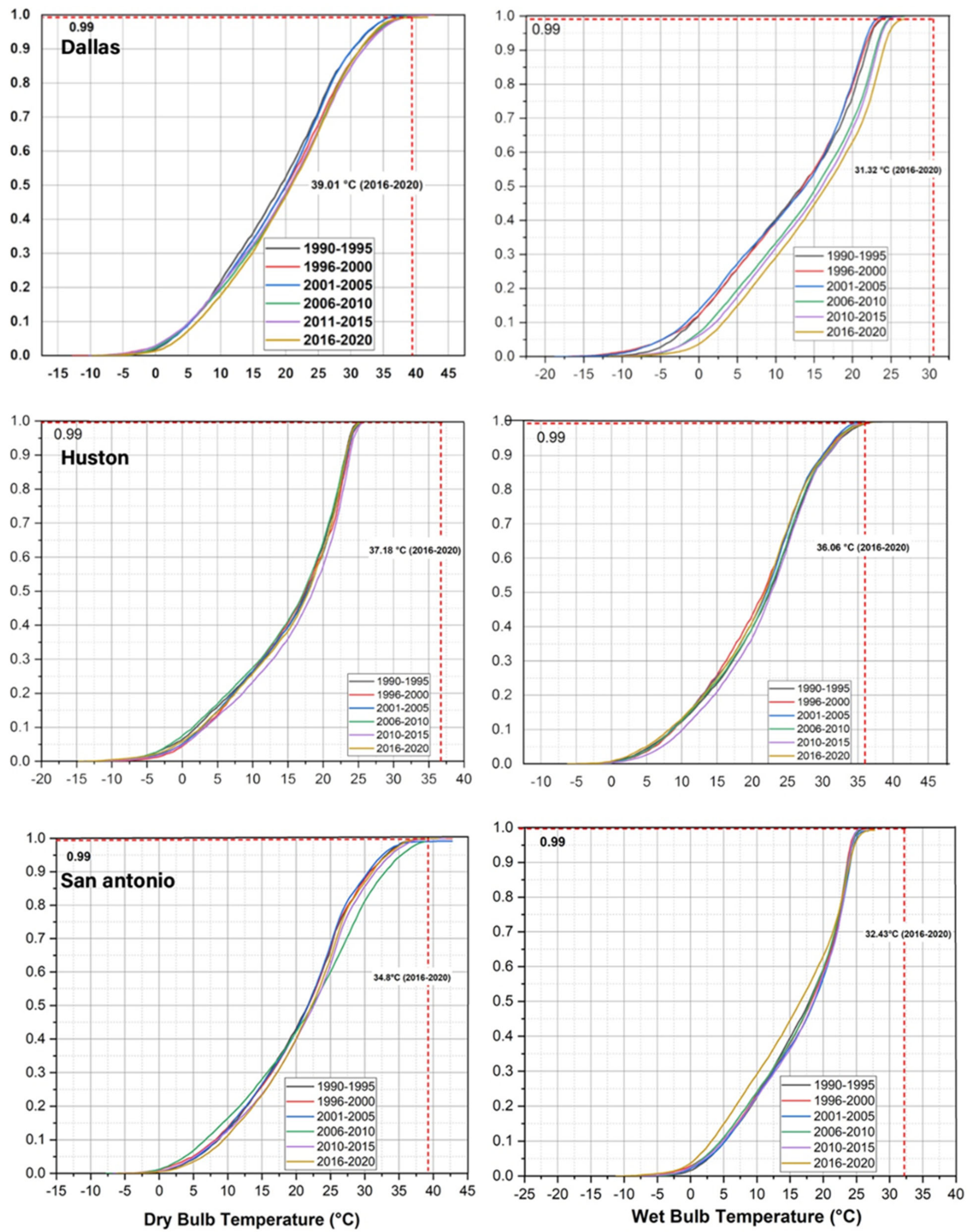
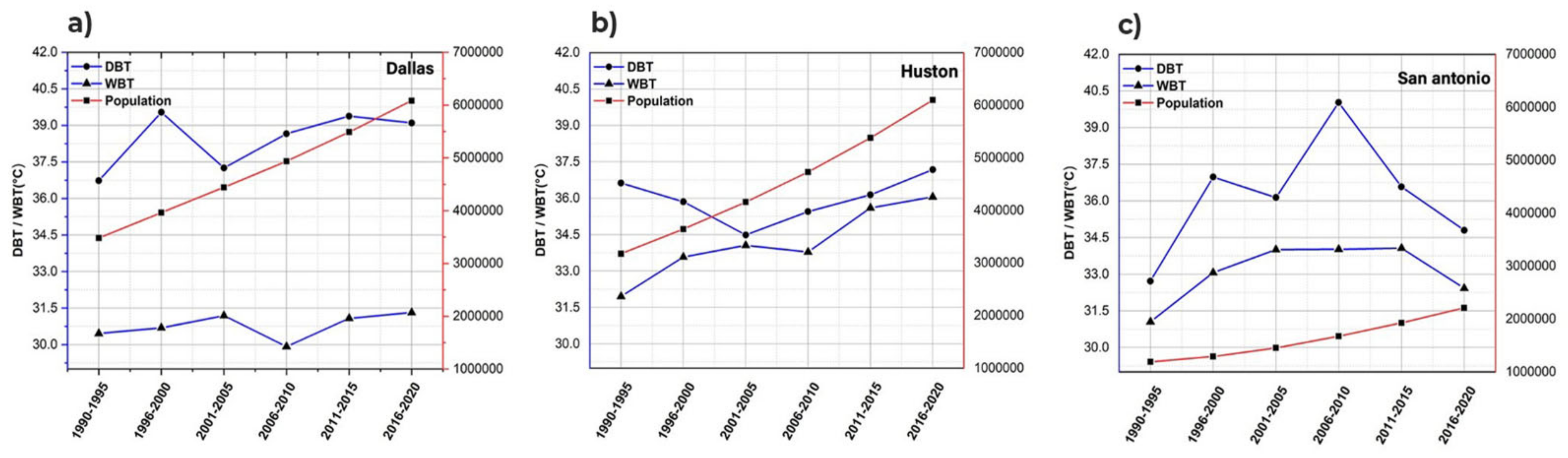
3.1. Outdoor Design Condition Evaluation in Terms of DBT and WBT Distribution

Because of modern lifestyles and migrant rural dwellers to urban areas, the global demand for energy required for cooling systems is increasing. This has a negative effect on the size of cities [55], urban health [56], and death rates due to heat and global warming [57,58]. Thus, choosing suitable cooling equipment with the highest energy performance has a significant impact on supporting a wide range of weather conditions [18]. As a result, the analysis and evaluation of outdoor design conditions appear to be more important than ever. The present study attempted to examine the climatic outdoor design conditions in terms of dry bulb temperature (DBT) and wet bulb temperature (WBT) in the three selected Texas cities between 1990 and 2020. Figure 3 illustrates the cumulative distribution function for DBT and WBT in selected cities between 1990–2020. As shown in Figure 3 and Table 1, based on 1% of the design conditions, the outdoor DBT for Dallas–Fort Worth, Houston, and San Antonio increased by 2.37 °C, 0.55 °C, and 2.06 °C, respectively, compared to the first review (1990–1995). Furthermore, the trend of increasing outdoor WBT conditions in these cities has been associated with the most significant increase in Houston (4.1 °C) and the lowest in Dallas–Fort Worth (0.86 °C). The rise in DBT and WBT in the selected cities also illustrates that the humidity ratio has increased in all cities; the highest and lowest increases in Houston (0.099 kg/kg) and Dallas–Fort Worth (0.008 kg/kg), respectively, have been reported. Thus, to create better thermal comfort in the subsequent years (2016–2020), the selected cities had to create more cooling loads than in the early years (1990–1995).
Based on 99% of climatic design conditions, the amount of DBT and WBT in the selected cities are quite interesting and opposite. The highest increases in DBT (2.19 °C) and WBT (1.34 °C) were recorded in Houston, while the lowest increases in DBT (0.39 °C) and WBT (0.92 °C) occurred in Dallas–Fort Worth. Conversely, the amount of DBT (−1.58 °C) and WBT (−1.66 °C) for San Antonio showed a decreasing trend between 1990 to 2020 (Figure 3 and Table 1), which correlates with some influential indexes such as demographic patterns on the variation of DBT and WBT (Figure 4). The design value for all conditions, including hot and cold seasons, for both DBT and WBT of the selected cities is depicted in Table 1.

3.2. Monthly Distribution of HDH, CDH, and NM Days during 1990–2020

The following section discusses the results of an analysis of the effect of climate change on the variation of CDH, CDH, and NM values from 1990 to 2020, as per ASHRAE, 2001 [38]. The analysis of temperature fluctuations in the selected cities during the study period indicates that the number of Cooling Degree Hours (CDH) has increased significantly while the number of Heating Degree Hours (HDH) has decreased (Table 2).
The effects of climate change on HDH fluctuations illustrate that the maximum decrease in HDH occurred in Dallas–Fort Worth (−2774.03-degree hours). In contrast, Houston (−510.66-degree hours) and San Antonio (−424.16-degree hours) reported fewer fluctuations in whole years and seasons. Therefore, it could be concluded that less heat energy was required in Houston and San Antonio cities than in Dallas–Fort Worth during 1990–2020. In spring and summer, however, the need for cooling systems has been felt more than before because of the reduction in NM fluctuations. The exponential growth of NM in autumn and winter over the last thirty years has revealed a decrease in heating energy demand (Table 2).
The effect of climate change on CDH has revealed that a tremendous increase in energy demand for cooling systems occurred in Dallas–Fort Worth among the selected cities between 1990 and 2020 (Table 2). Figure 5 indicates the heat map of selected cities’ CDH, HDH, and NM from 1990–2020. Based on the results in Figure 5, San Antonio grew by (254.56-degree hours) and Houston, which did not need cooling systems, was next in ranking. The achieved results highlighted the declining demand for cooling energy in San Antonio during winter, where the CDH decreased by 4.2-degree hours compared to 1991. On average, the NM fluctuations in the studied cities indicate a decrease in NM compared to earlier years. The highest and lowest decreases were observed in Dallas–Fort Worth and San Antonio, respectively (Figure 5).
The outcomes of the research indicate that climate change trends do not necessarily improve neutral mode conditions, and the energy consumption of buildings for space cooling has increased over time much more than for space heating. Indeed, the climate significantly impacts all vital parts of the energy industry, including energy consumption and electricity production. Warmer winter temperatures in cold climates may decrease energy consumption since less space heating will be necessary. Alternatively, increased summer temperatures in warmer climates will increase the energy needed to power air conditioners and refrigerators. These findings are consistent with the majority of previous studies. For instance: in Portugal, Gouveia et al., projected a potential variation in demand for space cooling energy services for 2050 ranging from 10% to +83% of current levels, depending on indoor thermal comfort conditions [59]. Their findings were corroborated by Figueiredo et al., who predicted that space cooling consumption could increase by a factor of 20 [59]. Therefore, choosing the right cooling equipment that has the highest energy efficiency with the lowest cost and covers a wide range of weather conditions is very important.

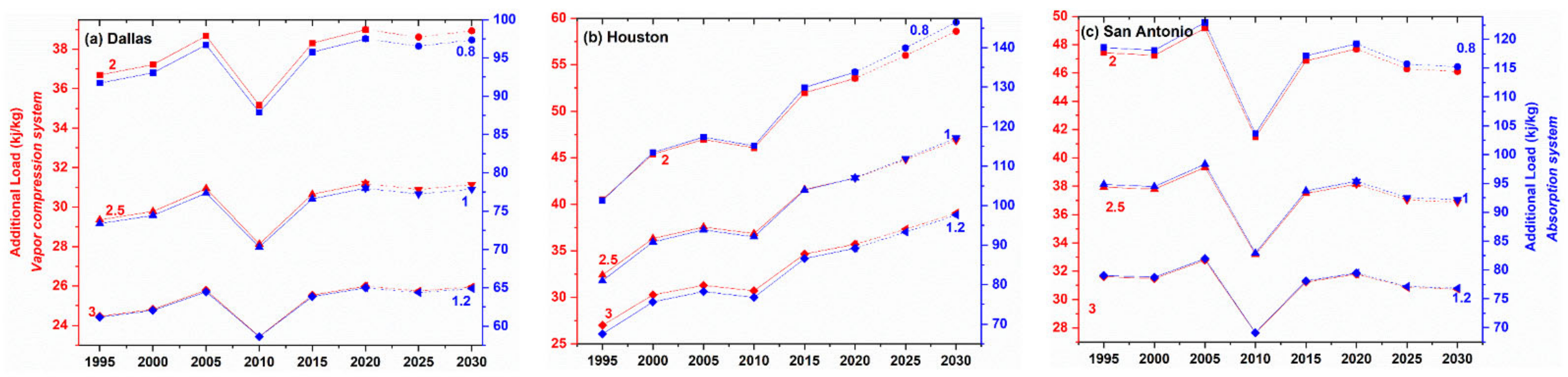
3.3. Evaluation of Cooling Systems

Climate change is regarded as the most serious threat to life on Earth. It is caused by natural and anthropogenic emissions of air pollutants, particularly greenhouse gases (GHGs), which have large-scale effects on the climate and, as a result, have an impact on all economic and societal levels, particularly in the energy sector. Energy systems, despite being one of the most important systems for social and economic development, frequently fail to account for the effects of climate change in their planning and operations. Paying attention to the effect of outdoor design conditions on selecting and sizing cooling equipment appears critical in this regard as a key element in controlling and aligning with the climate. Furthermore, given that the amount of Qcool is varied in each study period and in each city due to different outdoor conditions, the systems’ energy consumption has been different. Estimating the impact of climate change on the amount of energy required in each of the VC and Abs systems has been calculated and shown in Figure 6 and 7. The results illustrate that climate and demographic changes in the surveyed cities have caused the energy required by Abs and VC systems to change significantly compared to earlier years. Generally, these systems have demanded more energy in the last three decades of investigations. Given that increasing or decreasing COP affects the amount of energy required by each cooling system, the COP values considerably impact the amount of energy consumed and the size of the cooling systems. For instance, an Abs with COP = 1 utilized 4.61 kJ/kg, 26.03 kJ/kg, and 0.52 kJ/kg more energy in 2016–2020 than a similar system in 1990–1995 to prepare the same indoor air conditions in Dallas–Fort Worth, Houston, and San Antonio, respectively (Figure 6). In other words, the input energy consumption (Qgenerator) of absorption chiller systems has recorded the highest growth in the cities of Houston (32.13%) and Dallas (6.28%) between 1990 and 2020, respectively. While the amount of input energy consumption of absorption chiller systems in San Antonio has not had a considerable change (0.05%). However, when VC systems with COP = 2.5 were applied, the amount of extra energy required in the cities of Dallas–Fort Worth, Houston, and San Antonio increased by 1.84 kJ/kg, 10.41 kJ/kg, and 0.21 kJ/kg, respectively, compared to the period 1990–1995 (Figure 7). In another way, the amount of electricity consumed (Wvc) by compressors in such systems has grown by more than 29.34% and 7.14% in Houston and Dallas, respectively, between 1990 and 2020. However, significant change was not observed in San Antonio in this period. Our results have shown that the impact of this additional energy consumption on energy costs during the utilization period is not negligible and that this additional energy demand is higher in systems with lower COPs. Moreover, the role of implemented policies in reducing the total residential energy consumption in San Antonio has been considerable. However, we are not able to explore the underlying mechanism through which the regulations influence the residential energy use. Detailed information on market agents’ preferences, decisions and actions would allow us to further disentangle the influence of these regulations. This is left for future research. The COP process of the VC and Abs systems for the period of 1990–2020 in all selected cities is shown Figure 6 and Figure 7.

3.4. Prediction of Climate Change in Terms of DBT and WBT

The cooling system’s performance evaluation has been directly impacted by the outdoor design conditions, especially the outdoor design temperature values, as seen from the earlier result of this study. As a result, it is critical to understand the future scenarios of these weather parameters in order to select better cooling systems for long-term sustainability. As a result, the ARIMA model was used to predict these weather parameters in this study, which will aid in the preparation of better thermal comfort, as well as the understanding of future energy consumption. Future projections indicate significant population growth in the selected cities. Demographic changes foretell increases from 6.3 to 7.3 million in Dallas–Fort Worth, from 6.3 to 7.6 million in Houston, and from 2.3 to 2.8 million in San Antonio from 2020 to 2030. The behavior of DBT and WBT in future years is predicted to be quite exciting and inverse in selected cities. Over the years 2020–2030, DBT and WBT are predicted to rise significantly in Dallas–Fort Worth and Houston but will experience a decreasing trend in DBT (from 34.8 °C to 33.95 °C) and WBT (from 32.43 °C to 31.97 °C) in San Antonio. Predictions of DBT, WBT, and population up to 2030 for the three studied cities in Texas are shown in Figure 8.
The second part of the prediction process was the future performance prediction of the Abs and VC systems. As observed in Figure 9, the variations in outdoor design conditions change the performance and application of cooling systems. Based on the results, three different COP scenarios have been projected in both Abs (0.8, 1, and 1.2) and VC (2, 2.5, and 3) systems. For both systems, the amount of additional load required was significantly higher in 2030 compared to 2020 in Dallas–Fort Worth and Houston and more prominent in Houston than in Dallas–Fort Worth (Figure 9). The rate of additional energy is higher for COPAbs = 0.8 and COPVC = 2 compared to COPAbs = 1.2 and COPVC = 3 in Dallas–Fort Worth and Houston, respectively. Conversely, the amount of additional load required for cooling systems in San Antonio shows a decreasing trend in 2030 predictions. The decreasing rate was more significant in the COP of Abs = 0.8 and VC = 2 and least significant in the COP of Abs = 1.2 and VC = 3.
Our results have reported that, although many USA cities have adopted their national programs aimed at reducing greenhouse gas emissions, the control of temperature changes is different based on the capacity of each city and has a direct relationship with the policies governing societies that require a sufficient understanding of how agents behave and interact with others. Governments, as providers of public goods and services and holders of broad powers, implicitly have a stake in adaptation as far as it impacts the ability of the government to function effectively and address market failures. Future studies may explore the impact of climate change on the performance of cooling towers, which are strongly influenced by variations in temperature and humidity of the surrounding environment, as well as their impact on sociodemographic and environmental factors that change by context. The accurate quantification of the energy consumption of each cooling system with different COP for every number of specified people have been considered as a limitation of the research. Moreover, future research can investigate the effect of climate change on outdoor design conditions and its impact on the energy performance of cooling systems in industries and the ecosphere sectors.

4. Conclusions

The current research examined the climatic design conditions, the variations in CDH, HDH, and NM parameters, and the operation of cooling systems affected by climate change over a 30-year period (1990–2020) in the cities of Dallas–Fort Worth, Houston, and San Antonio, Texas. The climatic outdoor design conditions of 1% for the study period illustrated that the values of DBT and WBT for the cities of Dallas–Fort Worth, Houston, and San Antonio (2.37 °C, 0.55 °C, and 2.06 °C, respectively, for DBT) and (0.86 °C, 4.1 °C and 2.95 °C, respectively, for WBT) have increased compared to the first period of the research (1990–1995) and naturally have affected the amount of humidity, both sensible and latent loads. It has been projected that DBT will rise more prominently in Houston (from 37.18 °C to 37.56 °C), followed by Dallas–Fort Worth (from 39.1 °C to 39.57 °C), while San Antonio will experience a decreasing trend (from 34.81 °C to 33.95 °C).
On the other hand, WBT shows an increasing trend in Dallas–Fort Worth (from 31.32 °C to 31.38 °C) and, most significantly, in Houston (from 36.06 °C to 37.71 °C) from 2020 to 2030. The values of WBT in San Antonio will decrease from 32.43 °C to 31.97 °C. Therefore, meeting the peak load energy demands will be more challenging in Dallas–Fort Worth and Houston in the future because of the impact of population growth and climate change. However, improved energy efficiency revived by organizations and the private sector in San Antonio has resulted in declining DBT and WBT values. Although demographic change has been on the rise, causing anthropogenic heat. Indeed, the DBT and WBT have decreased in the last period of research (2016–2020) in San Antonio, despite the increase in population, which is considered an influential factor in increasing urban temperatures. Dallas–Fort Worth, on the other hand, experienced a trend decrease in DBT (2 °C) and WBT (0.5 °C) in 2000–2005 and 2005–2010, respectively. However, in both periods, a considerable increase in the population (more than 500,000 residents) was observed. This phenomenon also occurred in Houston in those same periods. Therefore, it can be concluded that population growth only partially affects the increase in DBT and WBT and there is no clear relationship between temperature increase and population trend in the studied cities, but other factors are effective in assessing urban temperatures. Furthermore, the effects of climate change on CDH and HDH values in the studied period indicated a significant decrease in HDH and an increase in CDH in the three studied cities. The largest drop in HDH was recorded in Dallas–Fort Worth, while there was less downward change in Houston and San Antonio in winter. In summer, however, the highest increase in CDH was reported in Dallas–Fort Worth, followed by San Antonio. It is predicted that by 2030, with the increase in population in the cities, the additional load required will significantly increase in Dallas–Fort Worth and Houston with both Abs and VC systems, while the additional load required for cooling systems in San Antonio will decrease. These changes indicate that although Dallas–Fort Worth has fewer residents than Houston, the recorded higher energy consumption and demographic changes as key elements of its increasing energy consumption do not have clear relationship with energy consumption and other factors that are also necessary to evaluate.

Author Contributions

Conceptualization, methodology, writing—original draft preparation, data curation, coding, investigation, visualization: A.K.; investigation, methodology: Y.J.K.; investigation, original draft preparation: N.M.Z.; Supervision and reviewing: A.G.-M.; Conceptualization, supervision, review and editing: S.D.; Supervision and reviewing: R.D.B.; Supervision: D.M.-R.; investigation, writing—original, Draw figures: P.M. All authors have read and agreed to the published version of the manuscript.

Funding

This research received no external funding.

Institutional Review Board Statement

Not applicable.

Informed Consent Statement

Not applicable.

Data Availability Statement

Data are available on request due to privacy/ethical restrictions.

Conflicts of Interest

The authors declare no conflict of interest.

References

  1. Zeng, A.; Ho, H.; Yu, Y. Prediction of building electricity usage using Gaussian Process Regression. J. Build. Eng. 2020, 28, 101054. [Google Scholar] [CrossRef]
  2. Hosseini, M.; Tardy, F.; Lee, B. Cooling and heating energy performance of a building with a variety of roof designs; the effects of future weather data in a cold climate. J. Build. Eng. 2018, 17, 107–114. [Google Scholar] [CrossRef] [Green Version]
  3. Jafarpur, P.; Berardi, U. Effects of climate changes on building energy demand and thermal comfort in Canadian office buildings adopting different temperature setpoints. J. Build. Eng. 2021, 42, 102725. [Google Scholar] [CrossRef]
  4. Nguyen, A.T.; Rockwood, D.; Doan, M.K.; Le, T.K.D. Performance assessment of contemporary energy-optimized office buildings under the impact of climate change. J. Build. Eng. 2021, 35, 102089. [Google Scholar] [CrossRef]
  5. Mariano-Hernández, D.; Hernández-Callejo, L.; Zorita-Lamadrid, A.; Duque-Pérez, O.; García, F.S. A review of strategies for building energy management system: Model predictive control, demand side management, optimization, and fault detect & diagnosis. J. Build. Eng. 2021, 33, 101692. [Google Scholar]
  6. Karimi, A.; Mohammad, P.; García-Martínez, A.; Moreno-Rangel, D.; Gachkar, D.; Gachkar, S. New developments and future challenges in reducing and controlling heat island effect in urban areas. Environ. Dev. Sustain. 2022, 1–47. [Google Scholar] [CrossRef]
  7. Huo, T.; Ma, Y.; Cai, W.; Liu, B.; Mu, L. Will the urbanization process influence the peak of carbon emissions in the building sector? A dynamic scenario simulation. Energy Build. 2021, 232, 110590. [Google Scholar] [CrossRef]
  8. Hu, Y.; Cheng, X.; Wang, S.; Chen, J.; Zhao, T.; Dai, E. Times series forecasting for urban building energy consumption based on graph convolutional network. Appl. Energy. 2022, 307, 118231. [Google Scholar] [CrossRef]
  9. Kyle, P.; Clarke, L.; Rong, F.; Smith, S.J. Climate policy and the long-term evolution of the US buildings sector. Energy J. Int. Assoc. Energy Econ. 2010, 31, 145–172. [Google Scholar]
  10. U.S. Energy Information Administration. State Energy Data System (SEDS): 1960–2019 (Complete): Consumption. U.S. Energy Inf. Adm. 2019. Available online: https://www.eia.gov/state/seds/seds-data-complete.php#Consumption&gt; (accessed on 2 February 2022).
  11. Birol, F. The Future of Cooling: Opportunities for Energy-Efficient Air Conditioning. International Energy Agency 2018. Available online: https://iea.blob.core.windows.net/assets/0bb45525-277f-4c9c-8d0c-9c0cb5e7d525/The_Future_of_Cooling.pdf (accessed on 26 January 2022).
  12. Davis, L.W.; Gertler, P.J. Contribution of air conditioning adoption to future energy use under global warming. Proc. Natl. Acad. Sci. USA 2015, 112, 5962–5967. [Google Scholar] [CrossRef] [Green Version]
  13. Karimi, A.; Mohammad, P. Effect of outdoor thermal comfort condition on visit of tourists in historical urban plazas of Sevilla and Madrid. Environ. Sci. Pollut. Res. 2022, 29, 60641–60661. [Google Scholar] [CrossRef]
  14. Karimi, A.; Mohammad, P.; Gachkar, S.; Gachkar, D.; García-Martínez, A.; Moreno-Rangel, D.; Brown, R.D. Surface Urban Heat Island Assessment of a Cold Desert City: A Case Study over the Isfahan Metropolitan Area of Iran. Atmosphere 2021, 12, 1368. [Google Scholar] [CrossRef]
  15. Belussi, L.; Barozzi, B.; Bellazzi, A.; Danza, L.; Devitofrancesco, A.; Fanciulli, C.; Ghellere, M.; Guazzi, G.; Meroni, I.; Salamone, F.; et al. A review of performance of zero energy buildings and energy efficiency solutions. J. Build. Eng. 2019, 25, 100772. [Google Scholar] [CrossRef]
  16. Lam, T.N.T.; Wan, K.K.W.; Wong, S.L.; Lam, J.C. Impact of climate change on commercial sector air conditioning energy consumption in subtropical Hong Kong. Appl. Energy 2010, 87, 2321–2327. [Google Scholar] [CrossRef]
  17. Losi, G.; Bonzanini, A.; Aquino, A.; Poesio, P. Analysis of thermal comfort in a football stadium designed for hot and humid climates by CFD. J. Build. Eng. 2021, 33, 101599. [Google Scholar] [CrossRef]
  18. Delfani, S.; Karami, M.; Pasdarshahri, H. The effects of climate change on energy consumption of cooling systems in Tehran. Energy Build. 2010, 42, 1952–1957. [Google Scholar] [CrossRef]
  19. Zhou, Y.; Eom, J.; Clarke, L. The effect of global climate change, population distribution, and climate mitigation on building energy use in the US and China. Clim. Change 2013, 119, 979–992. [Google Scholar] [CrossRef]
  20. Wang, H.; Chen, Q. Impact of climate change heating and cooling energy use in buildings in the United States. Energy Build. 2014, 82, 428–436. [Google Scholar] [CrossRef] [Green Version]
  21. Zhou, Y.; Clarke, L.; Eom, J.; Kyle, P.; Patel, P.; Kim, S.H.; Dirks, J.; Jensen, E.; Liu, Y.; Rice, J.; et al. Modeling the effect of climate change on US state-level buildings energy demands in an integrated assessment framework. Appl. Energy 2014, 113, 1077–1088. [Google Scholar] [CrossRef]
  22. Chakraborty, D.; Alam, A.; Chaudhuri, S.; Başağaoğlu, H.; Sulbaran, T.; Langar, S. Scenario-based prediction of climate change impacts on building cooling energy consumption with explainable artificial intelligence. Appl. Energy 2021, 291, 116807. [Google Scholar] [CrossRef]
  23. Ortiz, L.; González, J.E.; Lin, W. Climate change impacts on peak building cooling energy demand in a coastal megacity. Environ. Res. Lett. 2018, 13, 94008. [Google Scholar] [CrossRef]
  24. Troup, L.; Eckelman, M.J.; Fannon, D. Simulating future energy consumption in office buildings using an ensemble of morphed climate data. Appl. Energy 2019, 255, 113821. [Google Scholar] [CrossRef]
  25. Rhodes, J.D. Texas Electric Grid Sets New System-Wide All-Time Peak Demand Record, Twice; Forbes: Jersey, NJ, USA, 2018. [Google Scholar]
  26. Thevenard, D.J.; Humphries, R.G. The Calculation of Climatic Design Conditions in the 2005 ASHRAE Handbook—Fundamentals. ASHRAE Trans. 2005, 111, 457–466. [Google Scholar]
  27. Ahmed, A. Climate Change Will Drive Up Energy Use in Texas and Beyond. 2019. Available online: https://www.texasobserver.org/climate-change-will-drive-up-energy-use-in-texas-and-beyond/ (accessed on 29 January 2022).
  28. Boice, D.C.; Garza, M.E.; Holmes, S.E. The Urban Heat Island of San Antonio, Texas. Curr. Perspect. Environ. Clim. Chang. 2019, 2, 19–35. [Google Scholar]
  29. Moser, A.; Uhl, E.; Rötzer, T.; Biber, P.; Dahlhausen, J.; Lefer, B.; Pretzsch, H. Effects of climate and the urban heat island effect on urban tree growth in Houston. Open J. For. 2017, 7, 428–445. [Google Scholar] [CrossRef] [Green Version]
  30. Winguth, A.M.E.; Kelp, B. The urban heat island of the north-central Texas region and its relation to the 2011 severe Texas drought. J. Appl. Meteorol. Climatol. 2013, 52, 2418–2433. [Google Scholar] [CrossRef]
  31. Nielsen-Gammon, J.; Escobedo, J.; Ott, C.; Dedrick, J.; Van Fleet, A. Assessment of Historic and Future Trends of Extreme Weather in Texas, 1900–2036; Prevention Web: Geneva, Switzerland, 2020. [Google Scholar]
  32. U.S. Census Bureau. QuickFacts: Texas. 2020. Available online: https://www.census.gov/quickfacts/TX&gt; (accessed on 5 February 2022).
  33. U.S. Environmental Protection Agency. What Climate Change Means for Texas. 2016. Available online: https://www.epa.gov/sites/default/files/2016-09/documents/climate-change-tx.pdf&gt; (accessed on 5 February 2022).
  34. Reidmiller, D.R.; Avery, C.W.; Easterling, D.R.; Kunkel, K.E.; Lewis, K.L.M.; Maycock, T.K.; Stewart, B.C. Impacts, Risks, and Adaptation in the United States: Fourth National Climate Assessment; National Oceanic and Atmospheric Administration: Washington, DC, USA, 2017; Volume 2. [Google Scholar]
  35. National Weather Service. DFW Climate Narrative. 2020. Available online: https://www.weather.gov/fwd/dfw_normals&gt; (accessed on 5 February 2022).
  36. Lott, J.N. 7.8 the Quality Control of the Integrated Surface Hourly Database; American Meteorological Society: Seattle, WA, USA, 2004. [Google Scholar]
  37. Del Greco, S.A.; Lott, N.; Hawkins, K.; Baldwin, R.; Anders, D.D.; Ray, R.; Dellinger, D.; Jones, P.; Smith, F. J2.1 Surface Data Integration at NOAA’S National Climatic Data Center: Data Format, Processing, QC, and Product Generation. 2006. Available online: https://ams.confex.com/ams/Annual2006/techprogram/paper_100500.htm (accessed on 5 February 2022).
  38. Wang, S.K. Chapter 27: Climate Design Information. In ASHRAE Fundamentals Handbook 2001; American Society of Heating, Refrigerating and Air-Conditioning Engineers: Atlanta, GA, USA, 2001. [Google Scholar]
  39. ASHRAE. ASHRAE Fundamentals Handbook 2001; American Society of Heating, Refrigerating and Air-Conditioning Engineers: Atlanta, GA, USA, 2001. [Google Scholar]
  40. Castaño-Rosa, R.; Barrella, R.; Sánchez-Guevara, C.; Barbosa, R.; Kyprianou, I.; Paschalidou, E.; Thomaidis, N.; Dokupilova, D.; Gouveia, J.; Kádár, J.; et al. Cooling degree models and future energy demand in the residential sector. A seven-country case study. Sustainability 2021, 13, 2987. [Google Scholar] [CrossRef]
  41. Ledesma, G.; Nikolic, J.; Pons-Valladares, O. Co-simulation for thermodynamic coupling of crops in buildings. Case study of free-running schools in Quito, Ecuador. Build. Environ. 2022, 207, 108407. [Google Scholar] [CrossRef]
  42. Kumar, S.; Mathur, J.; Mathur, S.; Singh, M.K.; Loftness, V. An adaptive approach to define thermal comfort zones on psychrometric chart for naturally ventilated buildings in composite climate of India. Build Environ. 2016, 109, 135–153. [Google Scholar] [CrossRef] [Green Version]
  43. Teitelbaum, E.; Jayathissa, P.; Miller, C.; Meggers, F. Design with Comfort: Expanding the psychrometric chart with radiation and convection dimensions. Energy Build. 2020, 209, 109591. [Google Scholar] [CrossRef]
  44. Austin, T.U.; Department of Mechanical Engineering the University of Texas. Sol Cool Proc First SOLERAS Work April 1980, Univ Pet Miner Dhahran, Saudi Arab. United States-Saudi Arabian Joint Program for Cooperation in the Field of …. 1980; p. 245. Available online: https://www.nrel.gov/docs/legosti/old/4147.pdf (accessed on 5 February 2022).
  45. Habib, M.F.; Ali, M.; Sheikh, N.A.; Badar, A.W.; Mehmood, S. Building thermal load management through integration of solar assisted absorption and desiccant air conditioning systems: A model-based simulation-optimization approach. J. Build. Eng. 2020, 30, 101279. [Google Scholar] [CrossRef]
  46. Jani, D.B.; Mishra, M.; Sahoo, P.K. A critical review on application of solar energy as renewable regeneration heat source in solid desiccant–vapor compression hybrid cooling system. J. Build. Eng. 2018, 18, 107–124. [Google Scholar] [CrossRef]
  47. Jalalizadeh, M.; Fayaz, R.; Delfani, S.; Mosleh, H.J.; Karami, M. Dynamic simulation of a trigeneration system using an absorption cooling system and building integrated photovoltaic thermal solar collectors. J. Build. Eng. 2021, 43, 102482. [Google Scholar] [CrossRef]
  48. Scoccia, R.; Toppi, T.; Aprile, M.; Motta, M. Absorption and compression heat pump systems for space heating and DHW in European buildings: Energy, environmental and economic analysis. J. Build. Eng. 2018, 16, 94–105. [Google Scholar] [CrossRef]
  49. Khashei, M.; Bijari, M. A novel hybridization of artificial neural networks and ARIMA models for time series forecasting. Appl. Soft. Comput. 2011, 11, 2664–2675. [Google Scholar] [CrossRef]
  50. Salman, A.G.; Kanigoro, B. Visibility forecasting using autoregressive integrated moving average (ARIMA) models. Procedia Comput. Sci. 2021, 179, 252–259. [Google Scholar] [CrossRef]
  51. Reikard, G. Predicting solar radiation at high resolutions: A comparison of time series forecasts. Sol. Energy 2009, 83, 342–349. [Google Scholar] [CrossRef]
  52. Farhath, Z.A.; Arputhamary, B.; Arockiam, L. A survey on ARIMA forecasting using time series model. Int. J. Comput. Sci. Mob. Comput. 2016, 5, 104–109. [Google Scholar]
  53. Younes, M.K.; Nopiah, Z.M.; Basri, N.E.A.; Basri, H. Medium term municipal solid waste generation prediction by autoregressive integrated moving average. AIP Conf. Proc. 2014, 1613, 427–435. [Google Scholar]
  54. Ling, T.-Y.; Yen, N.; Lin, C.-H.; Chandra, W. Critical thinking in the urban living habitat: Attributes criteria and typo-morphological exploration of modularity design. J. Build. Eng. 2021, 44, 103278. [Google Scholar] [CrossRef]
  55. Kabisch, N.; Stadler, J.; Korn, H.; Bonn, A. Nature-Based Solutions to Climate Change Mitigation and Adaptation in Urban Areas–Perspectives on Indicators, Knowledge Gaps, Opportunities and Barriers for Action; BfN-Skripten: Malmö, Sweden, 2016. [Google Scholar]
  56. Akkose, G.; Akgul, C.M.; Dino, I.G. Educational building retrofit under climate change and urban heat island effect. J. Build. Eng. 2021, 40, 102294. [Google Scholar] [CrossRef]
  57. Mathur, U.; Damle, R. Impact of air infiltration rate on the thermal transmittance value of building envelope. J. Build. Eng. 2021, 40, 102302. [Google Scholar] [CrossRef]
  58. Gouveia, J.P.; Fortes, P.; Seixas, J. Projections of energy services demand for residential buildings: Insights from a bottom-up methodology. Energy 2012, 47, 430–442. [Google Scholar] [CrossRef]
  59. Figueiredo, R.; Nunes, P.; Panão, M.J.N.O.; Brito, M.C. Country residential building stock electricity demand in future climate–Portuguese case study. Energy Build. 2020, 209, 109694. [Google Scholar] [CrossRef]
Figure 1. Methodology flow diagram adopted in this study.
Sustainability 14 14848 g001
Figure 2. The location of Texas and our studies of cities in the United States.
Sustainability 14 14848 g002
Figure 3. The cumulative distribution function for dry bulb temperature and wet bulb temperature in Dallas, Houston and, San Antonio between 1990–2020.
Sustainability 14 14848 g003
Figure 4. The trend of changes in DBT, WBT, and population in the last 30 years (1990–2020) in Dallas (a), Houston (b), and San Antonio (c).
Sustainability 14 14848 g004
Figure 5. The heat map of CDH, HDH, and NM of selected cities in the period 1990–2020.
Sustainability 14 14848 g005
Figure 6. COP of absorption system at the selected cities between 1990–2020.
Sustainability 14 14848 g006
Figure 7. COP of vapor compression system at the selected cities between 1990–2020.
Sustainability 14 14848 g007
Figure 8. The prediction of demographic changed, DBT and WBT for Dallas (a), Houston (b) and San Antonio (c) (2020–2030).
Sustainability 14 14848 g008
Figure 9. Performance prediction of absorption and vapor compression cooling system in Dallas (a), Houston (b), and San Antonio (c) (2020–2030).
Sustainability 14 14848 g009
Table 1. Design values for the cold and hot seasons of Dallas, Houston, and San Antonio.
PeriodCityHeating DaysCooling Days
0.9960.990.0040.010.02
DBWBDBWBDBWBDBWBDBWB
1990–1995Dallas−1.25−9.36−1−9.1136.9630.6936.7330.4636.3530.06
1996–2000−3.44−9.44−3.18−9.239.8130.9439.5430.6939.1130.29
2001–2005−1.29−9.87−1.05−9.6237.4931.4437.2531.1936.8630.77
2006–2010−1.36−10.18−1.11−9.9338.930.1638.6629.9238.2529.51
2011–2015−2.15−10.81−1.89−10.5639.6331.3339.3831.0838.9630.65
2016–2020−0.84−8.43−0.61−8.1939.3431.5739.131.3238.6930.91
1990–1995Houston−3.35−5.39−4.02−5.1436.8935.8236.6331.9635.4431.62
1996–2000−1.05−5.86−0.83−5.636.1232.1735.8633.5833.6633.22
2001–2005−2.21−5.74−2.01−5.4934.2933.7934.4934.0635.0434.13
2006–2010−1.82−5.06−1.6−4.8235.734.7135.4533.7935.7333.42
2011–2015−1.69−5.7−1.47−5.4536.383436.1435.636.235.22
2016–2020−2.05−4.05−1.83−3.837.4336.3137.1836.0636.7635.64
1990–1995San Antonio0.02−2.020.2−1.8132.9331.2332.7231.0532.3730.73
1996–2000−0.63−1.63−0.4−1.4237.233.2836.9833.0736.5932.72
2001–2005−0.93−1.5−0.71−1.2836.3734.2236.1434.0135.7733.65
2006–20100.15−2.310.39−2.0840.2834.2440.0334.0239.6333.65
2011–2015−1.08−1.82−0.85−1.636.8134.2936.5834.0736.233.71
2016–2020−1.61−3.7−1.38−3.4835.0232.6534.832.4334.4332.06
Table 2. Fluctuations of CDH, HDH, and NM in different seasons of selected cities.
SeasonCity
DallasHoustonSan Antonio
SpringHDH−2215.1−363.95−263.05
NM−856−360.75−76.7
CDH634.50194.5
SummerHDH000
NM−4121.55−2967.7−2811.7
CDH3948.750699.7
AutumnHDH−2229.45−916.6−721.05
NM1032713.6941.7
CDH932.950128.25
WinterHDH−5286.3−762.1−712.55
NM4.71397.751802.35
CDH00−4.2
AnnualHDH−2774.03−510.663−424.163
NM−985.212−304.275−36.0875
CDH1379.050254.5625
Publisher’s Note: MDPI stays neutral with regard to jurisdictional claims in published maps and institutional affiliations.

