
Spatiotemporal Dynamics of Water Quality Indicators in Koka Reservoir, Ethiopia

 , , ,
, , ,  and
and
Abstract
1. Introduction
Related Work
2. Materials and Methods
2.1. Study Site
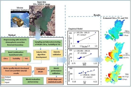
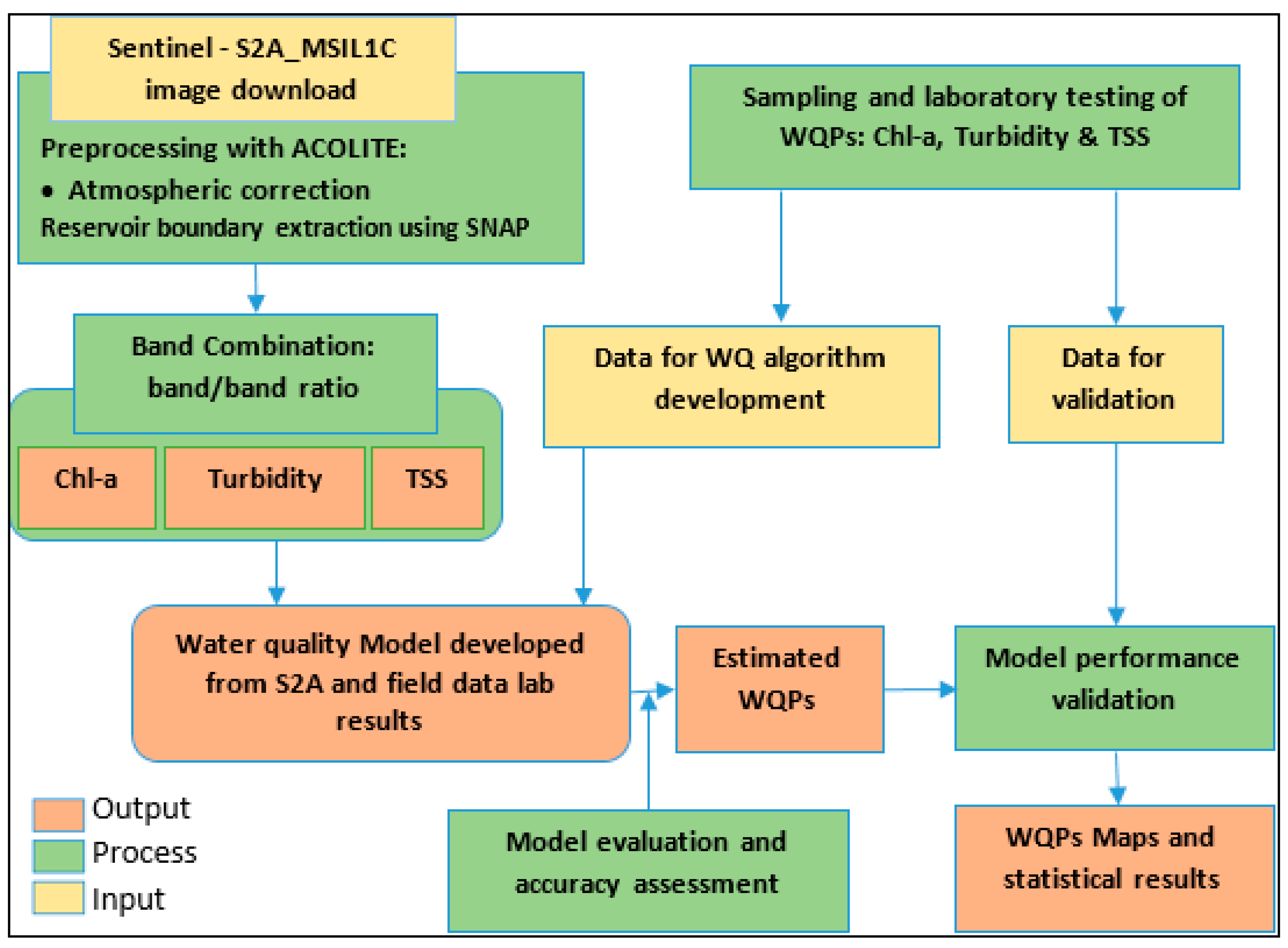
2.2. Methodology
2.2.1. In Situ Water Sampling and Laboratory Analysis
2.2.2. Atmospheric Correction (AC)
2.2.3. Sentinel-2 Analysis and Boundary Extraction
2.2.4. Empirical Analysis for the WQPs Model Development
3. Results
3.1. In Situ Data
3.2. Remote Sensing Reflectance Rrs (λ) in Sampling Locations
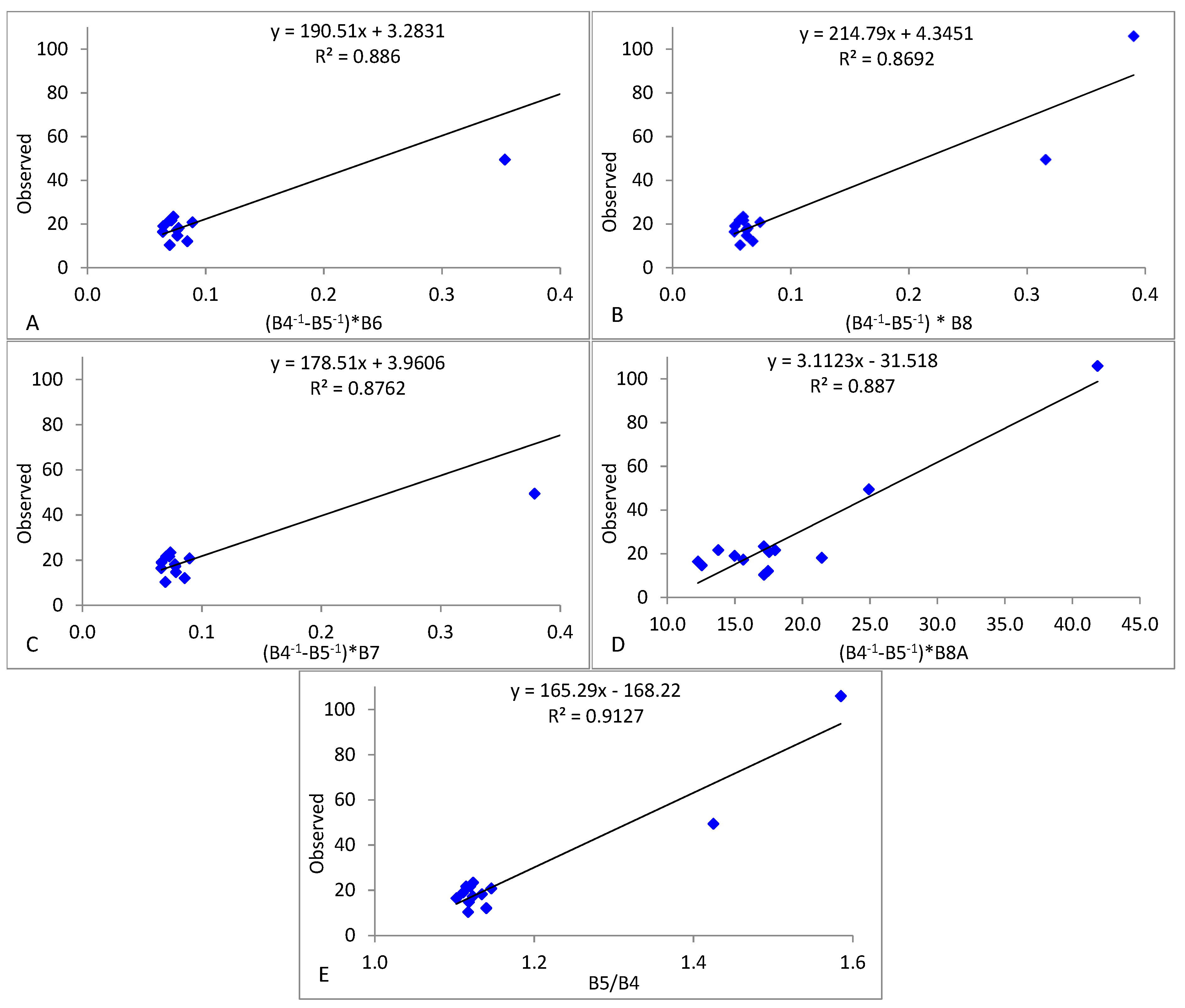
3.3. Empirical Model Development for Chlorophyll a
3.4. Empirical Model Development for Turbidity
3.5. Empirical Model Development for TSS
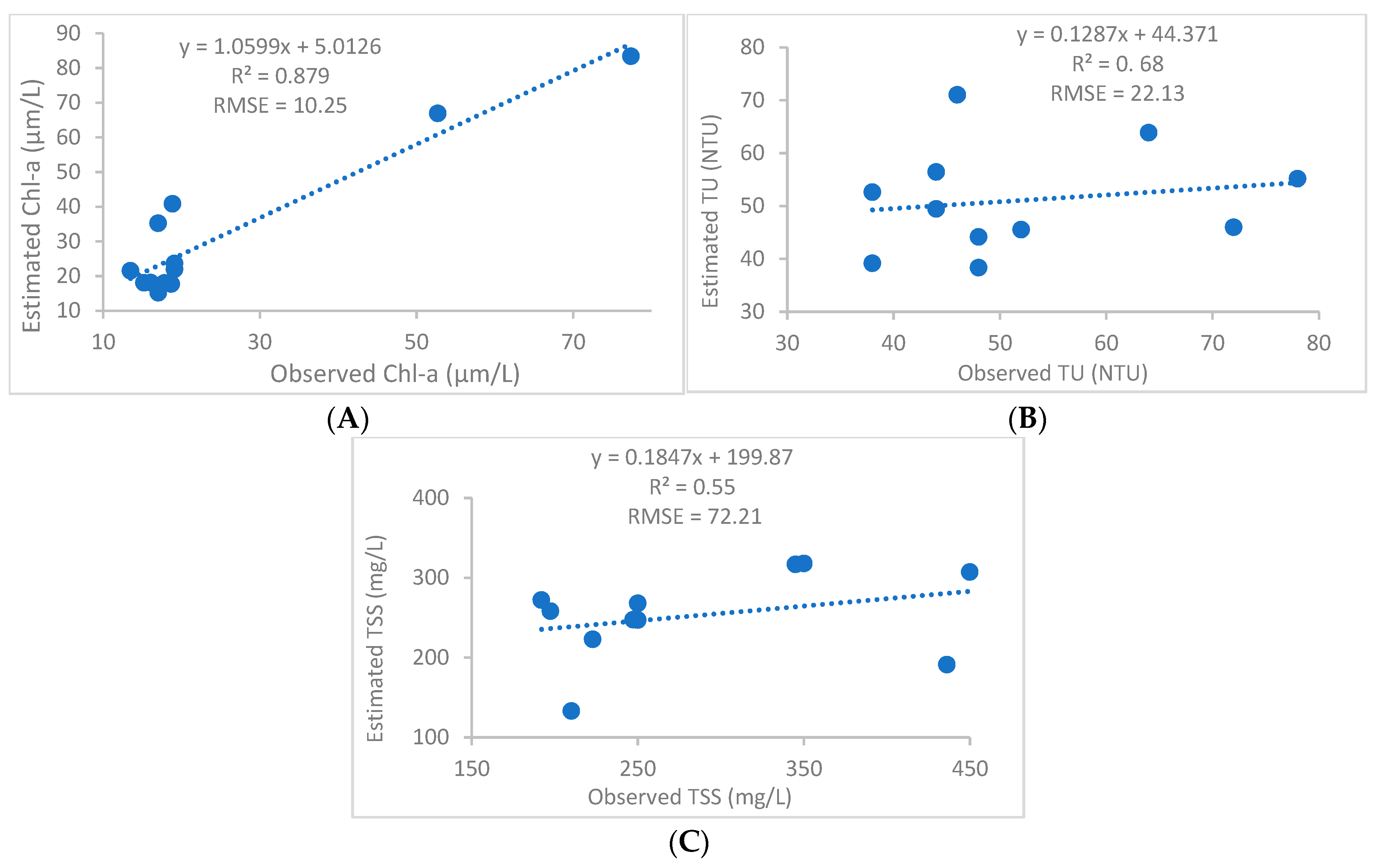
3.6. Model Performance Validation with In Situ Measurements
3.7. Spatial and Temporal Patterns of Water Quality Parameters Mapping
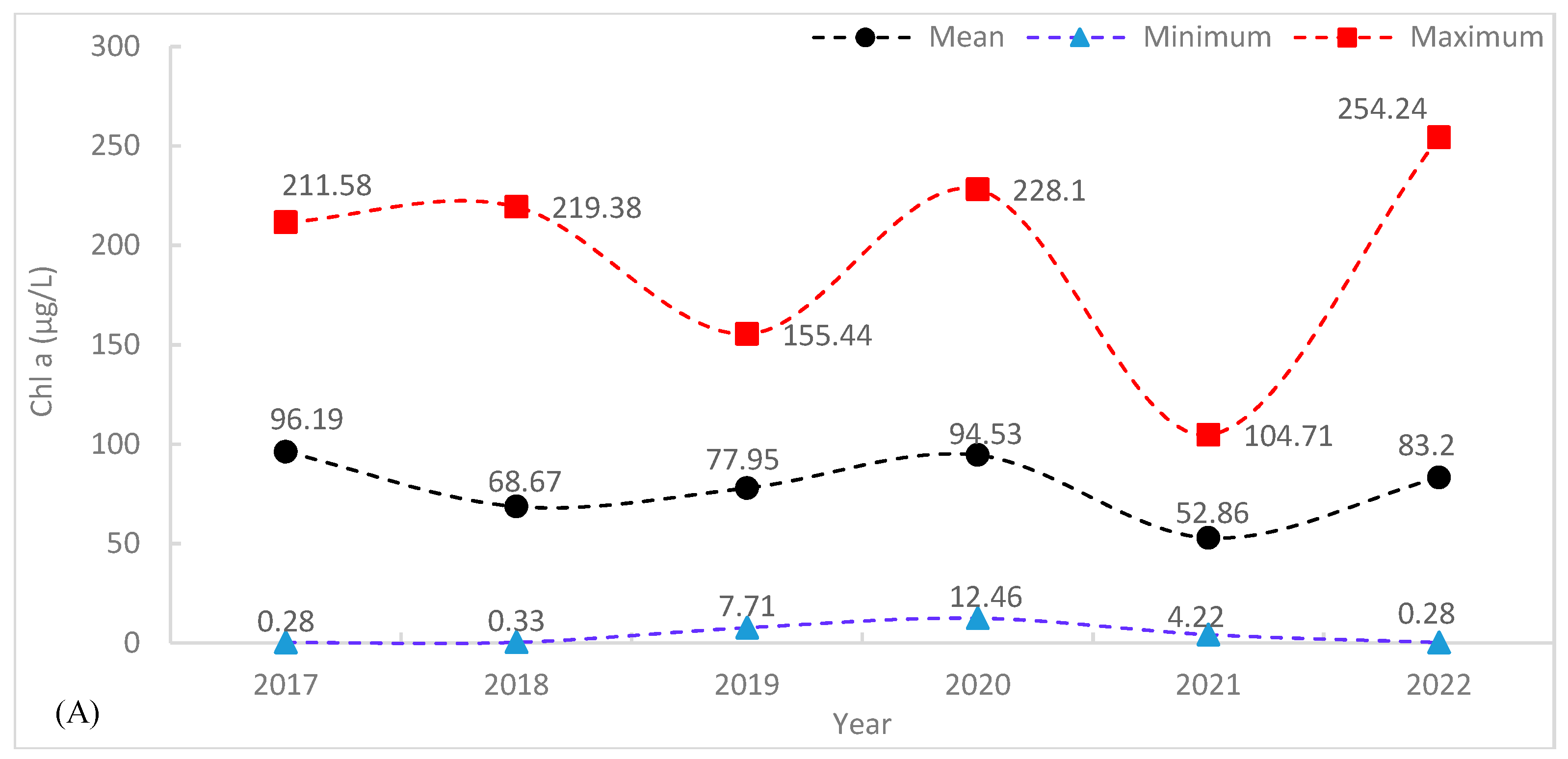
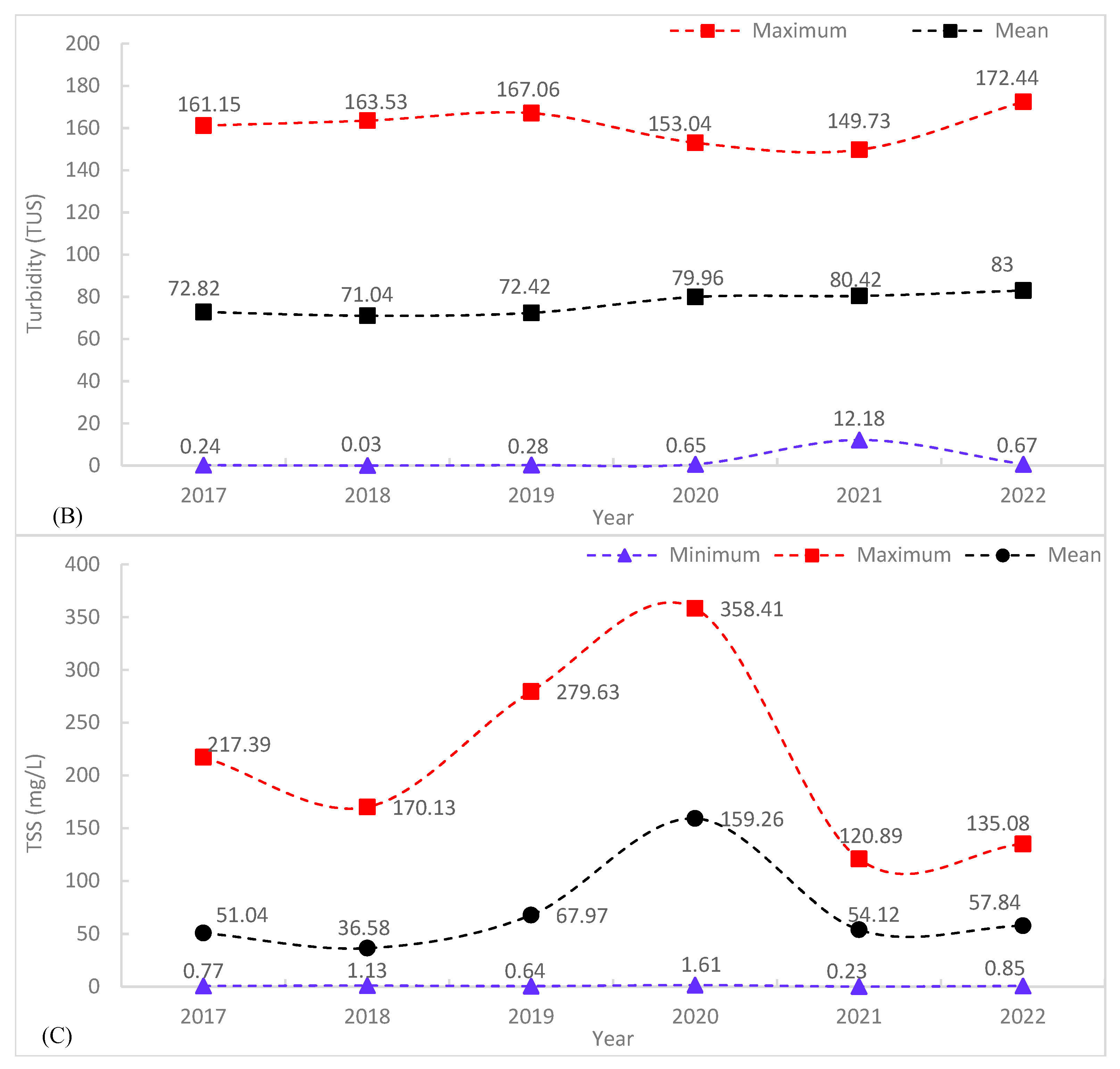
3.7.1. Temporal Variation of Water Quality Parameters
3.7.2. Spatial Distribution of Chl-a, TU, and TSS and Time Series Analysis
4. Discussion
5. Conclusions
Author Contributions
Funding
Data Availability Statement
Acknowledgments
Conflicts of Interest
Appendix A


References
- Mishra, A.K.; Singh, V.P. A review of drought concepts. J. Hydrol. 2010, 391, 202–216. [Google Scholar] [CrossRef]
- Chawla, I.; Karthikeyan, L.; Mishra, A.K. A review of remote sensing applications for water security: Quantity, quality, and extremes. J. Hydrol. 2020, 585, 124826. [Google Scholar] [CrossRef]
- UNEP. Progress on Ambient Water Quality. Tracking SDG 6 Series: Global Indicator 6.3.2 Updates and Acceleration Needs; UNEP: Nairobi, Kenya, 2021. [Google Scholar]
- Ademe, A.S. Source and Determinants of Water Pollution in Ethiopia: Distributed Lag Modeling Approach. Intellect. Prop. Rights Open Access 2014, 2. [Google Scholar] [CrossRef]
- Assegide, E.; Alamirew, T.; Dile, Y.T.; Bayabil, H.; Tessema, B.; Zeleke, G. A Synthesis of Surface Water Quality in Awash Basin, Ethiopia. Front. Water 2022, 4, 782124. [Google Scholar] [CrossRef]
- Abhachire, L.W. Studies on Hydrobiological Features of Koka Reservoir and Awash River in Ethiopia. Int. J. Fish. Aquat. Stud. 2014, 1, 158–162. Available online: www.fisheriesjournal.com (accessed on 10 September 2019).
- Assegide, E.; Alamirew, T.; Bayabil, H.; Dile, Y.T.; Tessema, B.; Zeleke, G. Impacts of Surface Water Quality in the Awash River Basin, Ethiopia: A Systematic Review. Front. Water 2022, 3, 790900. [Google Scholar] [CrossRef]
- Ligdi, E.E.; El Kahloun, M.; Meire, P. Ecohydrological status of Lake Tana—A shallow highland lake in the Blue Nile (Abbay) basin in Ethiopia: Review. Ecohydrol. Hydrobiol. 2010, 10, 109–122. [Google Scholar] [CrossRef]
- Abell, J.M.; Özkundakci, D.; Hamilton, D.P.; Jones, J.R. Latitudinal variation in nutrient stoichiometry and chlorophyll-nutrient relationships in lakes: A global study. Fundam. Appl. Limnol. 2012, 181, 1–14. [Google Scholar] [CrossRef]
- Alemu, M.L.; Geset, M.; Mosa, H.M.; Zemale, F.A.; Moges, M.A.; Giri, S.K.; Tillahun, S.A.; Melesse, A.; Ayana, E.K.; Steenhuis, T.S. Spatial and Temporal Trends of Recent Dissolved Phosphorus Concentrations in Lake Tana and its Four Main Tributaries. Land Degrad. Dev. 2017, 28, 1742–1751. [Google Scholar] [CrossRef]
- Maschal Tarekegn, M.; Truye, A.Z. Causes and impacts of shankila river water pollution in Addis Ababa, Ethiopia. Environ. Risk Assess. Remediat. 2018, 2, 21–30. Available online: http://www.alliedacademies.org/environmental-risk-assessment-and-remediation/ (accessed on 23 September 2019).
- Toming, K.; Kutser, T.; Laas, A.; Sepp, M.; Paavel, B.; Nõges, T. First experiences in mapping lake water quality parameters with sentinel-2 MSI imagery. Remote Sens. 2016, 8, 640. [Google Scholar] [CrossRef]
- Yepez, S.; Laraque, A.; Martinez, J.M.; De Sa, J.; Carrera, J.M.; Castellanos, B.; Gallay, M.; Lopez, J.L. Retrieval of suspended sediment concentrations using Landsat-8 OLI satellite images in the Orinoco River (Venezuela). Comptes Rendus Geosci. 2018, 350, 20–30. [Google Scholar] [CrossRef]
- Ismail, K.; Boudhar, A.; Abdelkrim, A.; Mohammed, H.; Mouatassime, S.; Kamal, A.O.; Driss, E.; Idrissi, E.A.; Nouaim, W. Evaluating the potential of Sentinel-2 satellite images for water quality characterization of artificial reservoirs: The Bin El Ouidane Reservoir case study (Morocco). Meteorol. Hydrol. Water Manag. Res. Oper. Appl. 2019, 7, 31–39. [Google Scholar] [CrossRef]
- Mamun, M.; Ferdous, J.; An, K.G. Empirical estimation of nutrient, organic matter and algal chlorophyll in a drinking water reservoir using landsat 5 tm data. Remote Sens. 2021, 13, 2256. [Google Scholar] [CrossRef]
- Ansper, A.; Alikas, K. Retrieval of Chlorophyll a from Sentinel-2 MSI Data for the European Union Water Framework Directive Reporting Purposes. Remote Sens. 2019, 11, 64. [Google Scholar] [CrossRef]
- Giardino, C.; Bresciani, M.; Villa, P.; Martinelli, A. Application of Remote Sensing in Water Resource Management: The Case Study of Lake Trasimeno, Italy. Water Resour. Manag. 2010, 24, 3885–3899. [Google Scholar] [CrossRef]
- Zhao, J.; Zhang, F.; Chen, S.; Wang, C.; Chen, J.; Zhou, H.; Xue, Y. Remote Sensing Evaluation of Total Suspended Solids Dynamic with Markov Model: A Case Study of Inland Reservoir across Administrative Boundary in South China. Sensors 2020, 20, 6911. [Google Scholar] [CrossRef]
- Wang, M.; Yao, Y.; Shen, Q.; Gao, H.; Li, J.; Zhang, F.; Wu, Q. Time-Series Analysis of Surface-Water Quality in Xiong’an New Area, 2016–2019. J. Indian Soc. Remote Sens. 2021, 49, 857–872. [Google Scholar] [CrossRef]
- Pizani, F.M.C.; Maillard, P.; Ferreira, A.F.F.; de Amorim, C.C.; Federal, U.; Gerais, D.M.; Horizonte, B.; Federal, U.; Gerais, D.M.; Horizonte, B.; et al. Estimation of Water Quality in a Reservoir from Sentinel-2 MSI and Landsat-8 Oli Sensors. ISPRS Ann. Photogramm. Remote Sens. Spat. Inf. Sci. 2020, 3, 401–408. [Google Scholar] [CrossRef]
- Govedarica, M.; Jakovljevic, G. Monitoring spatial and temporal variation of water quality parameters using time series of open multispectral data. In Proceedings of the Proc. SPIE 11174, Seventh International Conference on Remote Sensing and Geoinformation of the Environment (RSCy2019), Paphos, Cyprus, 27 June 2019; p. 55. [Google Scholar] [CrossRef]
- Masresha, A.E.; Skipperud, L.; Rosseland, B.O.; Zinabu, G.M.; Meland, S.; Teien, H.C.; Salbu, B. Speciation of selected trace elements in three ethiopian rift valley lakes (koka, ziway, and awassa) and their major inflows. Sci. Total Environ. 2011, 409, 3955–3970. [Google Scholar] [CrossRef]
- Mesfin, M.; Tudorancea, C.; Baxter, R.M. Some limnological observations on two Ethiopian hydroelectric reservoirs: Koka (Shewa administrative district) and Finchaa (Welega administrative district). Hydrobiologia 1988, 157, 47–55. [Google Scholar] [CrossRef]
- Fasil, D.; Kibru, T.; Gashaw, T.; Fikadu, T.; Aschalew, D. Some limnological aspects of Koka reservoir, a shallow tropical artificial lake, Ethiopia. J. Recent Trends Biosci. 2011, 1, 94–100. [Google Scholar]
- Tesfay, H. Spatio-Temporal Variations of the Biomass and Primary Production of Phytoplankton in Koka Reservoir; Addis Ababa University, Collage of Natural Sciences: Addis Ababa, Ethiopia, 2007. [Google Scholar]
- Topp, S.N.; Pavelsky, T.M.; Jensen, D.; Simard, M.; Ross, M.R.V. Research trends in the use of remote sensing for inland water quality science: Moving towards multidisciplinary applications. Water 2020, 12, 169. [Google Scholar] [CrossRef]
- Sent, G.; Biguino, B.; Favareto, L.; Cruz, J.; Sá, C.; Dogliotti, A.I.; Palma, C.; Brotas, V.; Brito, A.C. Deriving water quality parameters using sentinel-2 imagery: A case study in the Sado Estuary, Portugal. Remote Sens. 2021, 13, 1043. [Google Scholar] [CrossRef]
- Buma, W.G.; Lee, S.I. Evaluation of Sentinel-2 and Landsat 8 images for estimating Chlorophyll-a concentrations in Lake Chad, Africa. Remote Sens. 2020, 12, 2437. [Google Scholar] [CrossRef]
- Lins, R.C.; Martinez, J.M.; Marques, D.D.M.; Cirilo, J.A.; Fragoso, C.R. Assessment of chlorophyll-a remote sensing algorithms in a productive tropical estuarine-lagoon system. Remote Sens. 2017, 9, 516. [Google Scholar] [CrossRef]
- Borges, H.D.; Cicerelli, R.E.; De Almeida, T.; Roig, H.L.; Olivetti, D. Monitoring cyanobacteria occurrence in freshwater reservoirs using semi-analytical algorithms and orbital remote sensing. Mar. Freshw. Res. 2020, 71, 569–578. [Google Scholar] [CrossRef]
- Subiyanto, S.; Ramadhanis, Z.; Baktiar, A.H. Integration of Remote Sensing Technology Using Sentinel-2A Satellite images for Fertilization and Water Pollution Analysis in Estuaries Inlet of Semarang Eastern Flood Canal. E3S Web Conf. 2018, 31, 12008. [Google Scholar] [CrossRef]
- Kupssinskü, L.S.; Guimarães, T.T.; De Souza, E.M.; Zanotta, D.C.; Veronez, M.R.; Gonzaga, L.; Mauad, F.F. A method for chlorophyll-a and suspended solids prediction through remote sensing and machine learning. Sensors 2020, 20, 2125. [Google Scholar] [CrossRef]
- Malthus, T.J.; Hestir, E.L.; Dekker, A.G.; Brando, V.E. The case for a global inland water quality product. In Proceedings of the 2012 IEEE International Geoscience and Remote Sensing Symposium, Munich, Germany, 22–27 July 2012; pp. 5234–5237. [Google Scholar]
- Schalles, J.F. Optical remote sensing techniques to estimate phytoplankton chlorophyll a concentrations in coastal waters with varying suspended matter and cdom concentrations. In Remote Sensing and Digital Image Processing; Springer: Berlin/Heidelberg, Germany, 2006; Volume 9, pp. 27–79. [Google Scholar]
- Cairo, C.; Barbosa, C.; Lobo, F.; Novo, E.; Carlos, F.; Maciel, D.; Jnior, R.F.; Silva, E.; Curtarelli, V. Hybrid chlorophyll-a algorithm for assessing trophic states of a tropical brazilian reservoir based on msi/sentinel-2 data. Remote Sens. 2019, 12, 40. [Google Scholar] [CrossRef]
- Ha, N.T.T.; Thao, N.T.P.; Koike, K.; Nhuan, M.T. Selecting the best band ratio to estimate chlorophyll-a concentration in a tropical freshwater lake using sentinel 2A images from a case study of Lake Ba Be (Northern Vietnam). ISPRS Int. J. Geo-Inf. 2017, 6, 290. [Google Scholar] [CrossRef]
- Mishra, S.; Mishra, D.R. Normalized difference chlorophyll index: A novel model for remote estimation of chlorophyll-a concentration in turbid productive waters. Remote Sens. Environ. 2012, 117, 394–406. [Google Scholar] [CrossRef]
- Ouma, Y.O.; Noor, K.; Herbert, K. Modelling Reservoir Chlorophyll-a, TSS, and Turbidity Using Sentinel-2A MSI and Landsat-8 OLI Satellite Sensors with Empirical Multivariate Regression. J. Sens. 2020, 2020, 8858408. [Google Scholar] [CrossRef]
- Rodríguez-Benito, C.V.; Navarro, G.; Caballero, I. Using Copernicus Sentinel-2 and Sentinel-3 data to monitor harmful algal blooms in Southern Chile during the COVID-19 lockdown. Mar. Pollut. Bull. 2020, 161, 111722. [Google Scholar] [CrossRef]
- Grendaitė, D.; Stonevičius, E.; Karosienė, J.; Savadova, K.; Kasperovičienė, J. Chlorophyll-a concentration retrieval in eutrophic lakes in Lithuania from Sentinel-2 data. Geol. Geogr. 2018, 4. [Google Scholar] [CrossRef]
- Quang, N.H.; Sasaki, J.; Higa, H.; Huan, N.H. Spatiotemporal variation of turbidity based on landsat 8 OLI in Cam Ranh Bay and Thuy Trieu Lagoon, Vietnam. Water 2017, 9, 570. [Google Scholar] [CrossRef]
- Ma, Y.; Song, K.; Wen, Z.; Liu, G.; Shang, Y.; Lyu, L.; Du, J.; Yang, Q.; Li, S.; Tao, H.; et al. Remote sensing of turbidity for lakes in Northeast China using sentinel-2 images with machine learning algorithms. IEEE J. Sel. Top. Appl. Earth Obs. Remote Sens. 2021, 14, 9132–9146. [Google Scholar] [CrossRef]
- Premkumar, R.; Venkatachalapathy, R.; Visweswaran, S. Mapping of Total Suspended Matter based on Sentinel-2 data on the Hooghly River, India. Indian J. Ecol. 2021, 48, 159–165. Available online: https://www.researchgate.net/profile/Prem-Kumar-82/publication/349683336_Mapping_of_Total_Suspended_Matter_based_on_Sentinel-2_data_on_the_Hooghly_River_India/links/603c6c98299bf1cc26fbd606/Mapping-of-Total-Suspended-Matter-based-on-Sentinel-2-data-on-the (accessed on 8 July 2021).
- Sòria-Perpinyà, X.; Vicente, E.; Urrego, P.; Pereira-Sandoval, M.; Tenjo, C.; Ruíz-Verdú, A.; Delegido, J.; Soria, J.M.; Peña, R.; Moreno, J. Validation of water quality monitoring algorithms for sentinel-2 and sentinel-3 in mediterranean inland waters with in situ reflectance data. Water 2021, 13, 686. [Google Scholar] [CrossRef]
- Liu, H.; Li, Q.; Shi, T.; Hu, S.; Wu, G.; Zhou, Q. Application of Sentinel 2 MSI Images to Retrieve Suspended Particulate Matter Concentrations in Poyang Lake. Remote Sens. 2017, 9, 761. [Google Scholar] [CrossRef]
- Caballero, I.; Steinmetz, F.; Navarro, G. Evaluation of the first year of operational Sentinel-2A data for retrieval of suspended solids in medium- to high-turbiditywaters. Remote Sens. 2018, 10, 982. [Google Scholar] [CrossRef]
- Nguyen, T.H.D.; Phan, K.D.; Nguyen, H.T.T.; Tran, S.N.; Tran, T.G.; Tran, B.L.; Doan, T.N. Total Suspended Solid Distribution in Hau River Using Sentinel 2A Satellite Imagery. ISPRS Ann. Photogramm. Remote Sens. Spat. Inf. Sci. 2020, 6, 91–97. [Google Scholar] [CrossRef]
- Dierssen, H.M.; Kudela, R.M.; Ryan, J.P.; Zimmerman, R.C. Red and black tides: Quantitative analysis of water-leaving radiance and perceived color for phytoplankton, colored dissolved organic matter, and suspended sediments. Limnol. Oceanogr. 2006, 51, 2646–2659. [Google Scholar] [CrossRef]
- Gitelson, A.; Mayo, M.; Yacobi, Y.Z.; Parparov, A.; Berman, T. The use of high-spectral-resolution radiometer data for detection of low chlorophyll concentrations in Lake Kinneret. J. Plankton Res. 1994, 16, 993–1002. [Google Scholar] [CrossRef]
- Matthews, M.W.; Bernard, S.; Robertson, L. An algorithm for detecting trophic status (chlorophyll-a), cyanobacterial-dominance, surface scums and floating vegetation in inland and coastal waters. Remote Sens. Environ. 2012, 124, 637–652. [Google Scholar] [CrossRef]
- Gower, J.; King, S.; Borstad, G.; Brown, L. Detection of intense plankton blooms using the 709 nm band of the MERIS imaging spectrometer. Int. J. Remote Sens. 2005, 26, 2005–2012. [Google Scholar] [CrossRef]
- Gitelson, A. The peak near 700 nm on radiance spectra of algae and water: Relationships of its magnitude and position with chlorophyll concentration. Int. J. Remote Sens. 1992, 13, 3367–3373. [Google Scholar] [CrossRef]
- Gholizadeh, M.H.; Melesse, A.M.; Reddi, L. A comprehensive review on water quality parameters estimation using remote sensing techniques. Sensors 2016, 16, 1298. [Google Scholar] [CrossRef]
- Martinez, J.-M.; Espinoza-Villar, R.; Armijos, E.; Moreira, L. The optical properties of river and floodplain waters in the Amazon River Basin: Implications for satellite-based measurements of suspended particulate matter. J. Geophys. Res. Earth Surf. 2015, 120, 1274–1287. [Google Scholar] [CrossRef]
- Marinho, R.R.; Harmel, T.; Martinez, J.M.; Filizola Junior, N.P. Spatiotemporal dynamics of suspended sediments in the negro river, amazon basin, from in situ and sentinel-2 remote sensing data. ISPRS Int. J. Geo-Inf. 2021, 10, 86. [Google Scholar] [CrossRef]
- SWECO. Review of Hydropower Multipurpose Project Coordination Regimes. 2008. Available online: http://nilebasin.org/nileis/system/files/NBI_BestPracticeCompendium_Final.pdf (accessed on 22 July 2022).
- Adane, G.B.; Hirpa, B.A.; Song, C.; Lee, W.K. Rainfall characterization and trend analysis of wet spell length across varied landscapes of the upper awash river basin, ethiopia. Sustainability 2020, 12, 9221. [Google Scholar] [CrossRef]
- Gebremichael, H.B.; Raba, G.A.; Beketie, K.T.; Feyisa, G.L.; Siyoum, T. Changes in daily rainfall and temperature extremes of upper Awash Basin, Ethiopia. Sci. Afr. 2022, 16, e01173. [Google Scholar] [CrossRef]
- Legese, W.; Koricha, D.; Ture, K. Characteristics of Seasonal Rainfall and its Distribution Over Bale Highland, Southeastern Ethiopia. J. Earth Sci. Clim. Chang. 2018, 9, 1–6. [Google Scholar] [CrossRef]
- Duguma, F.A.; Feyessa, F.F.; Demissie, T.A.; Januszkiewicz, K. Hydroclimate trend analysis of upper awash basin, Ethiopia. Water 2021, 13, 1680. [Google Scholar] [CrossRef]
- WILDCO. A Comprehensive Guide to Wildco Water Bottle Samplers. 2013, pp. 1–14. Available online: https://wildco.com/wp-content/uploads/2017/05/1200-G-Kemmerer.pdf (accessed on 11 July 2022).
- EPA ESS Method 150.1: Chlorophyll—Spectrophotometric 1991. no. September. Environmental Sciences Section Inorganic Chemistry Unit Wisconsin State Lab of Hygiene 465 Henry Mall Madison, WI 53706. 1991. Available online: http://polk.wateratlas.usf.edu/upload/documents/methd150.pdf (accessed on 11 July 2022).
- Vanhellemont, Q.; Ruddick, K. Acolite for Sentinel-2: Aquatic applications of MSI imagery. In Proceedings of the 2016 ESA Living Planet Symposium, Prague, Czech Republic, 9–13 May 2016. [Google Scholar]
- Saberioon, M.; Brom, J.; Nedbal, V.; Souček, P.; Císař, P. Chlorophyll-a and total suspended solids retrieval and mapping using Sentinel-2A and machine learning for inland waters. Ecol. Indic. 2020, 113, 106236. [Google Scholar] [CrossRef]
- Angelats, E.; Fern, M. First Results of Phytoplankton Spatial Dynamics in Two NW-Mediterranean Bays from Chlorophyll- a Estimates Using Sentinel 2: Potential Implications for Aquaculture. Remote Sens. 2019, 11, 1756. [Google Scholar]
- Vanhellemont, Q. Adaptation of the dark spectrum fitting atmospheric correction for aquatic applications of the Landsat and Sentinel-2 archives. Remote Sens. Environ. 2019, 225, 175–192. [Google Scholar] [CrossRef]
- Molkov, A.A.; Fedorov, S.V.; Pelevin, V.V.; Korchemkina, E.N. Regional models for high-resolution retrieval of chlorophyll a and TSM concentrations in the Gorky Reservoir by Sentinel-2 imagery. Remote Sens. 2019, 11, 1215. [Google Scholar] [CrossRef]
- Warren, M.A.; Simis, S.G.H.; Martinez-Vicente, V.; Poser, K.; Bresciani, M.; Alikas, K.; Spyrakos, E.; Giardino, C.; Ansper, A. Assessment of atmospheric correction algorithms for the Sentinel-2A MultiSpectral Imager over coastal and inland waters. Remote Sens. Environ. 2019, 225, 267–289. [Google Scholar] [CrossRef]
- Xu, H. Modification of normalised difference water index (NDWI) to enhance open water features in remotely sensed imagery. Int. J. Remote Sens. 2006, 27, 3025–3033. [Google Scholar] [CrossRef]
- Singh, K.V.; Setia, R.; Sahoo, S.; Prasad, A.; Pateriya, B. Evaluation of NDWI and MNDWI for assessment of waterlogging by integrating digital elevation model and groundwater level. Geocarto Int. 2015, 30, 650–661. [Google Scholar] [CrossRef]
- Lai, Y.; Zhang, J.; Song, Y.; Gong, Z. Retrieval and evaluation of chlorophyll-a concentration in reservoirs with main water supply function in beijing, china, based on landsat satellite images. Int. J. Environ. Res. Public Health 2021, 18, 4419. [Google Scholar] [CrossRef] [PubMed]
- Jaelani, L.M.; Limehuwey, R.; Kurniadin, N.; Pamungkas, A.; Koenhardono, E.S.; Sulisetyono, A. Estimation of Total Suspended Sediment and Chlorophyll-A Concentration from Landsat 8-Oli: The Effect of Atmospher and Retrieval Algorithm. IPTEK J. Technol. Sci. 2016, 27, 16–23. [Google Scholar] [CrossRef]
- Bryant, M.A.; Hesser, T.J.; Jensen, R.E. Evaluation Statistics Computed for the Wave Information Studies (WIS). 2016, pp. 1–10. Available online: https://apps.dtic.mil/sti/citations/AD1013235 (accessed on 25 April 2022).
- Ruddick, K.; Nechad, B.; Neukermans, G.; Park, Y.; Doxaran, D.; Sirjacobs, D.; Beckers, J.-M. Remote Sensing of Suspended Particulate Matter in Turbid Waters: State of the Art and Future Perspectives. In Proceedings of the Ocean Optics XIX Conference, Barga, Italy, 6–10 October 2008. [Google Scholar]
- Katlane, R.; Dupouy, C.; El Kilani, B.; Berges, J.C. Estimation of Chlorophyll and Turbidity Using Sentinel 2A and EO1 Data in Kneiss Archipelago Gulf of Gabes, Tunisia. Int. J. Geosci. 2020, 11, 708–728. [Google Scholar] [CrossRef]
- Matthews, M.W.; Bernard, S.; Winter, K. Remote sensing of cyanobacteria-dominant algal blooms and water quality parameters in Zeekoevlei, a small hypertrophic lake, using MERIS. Remote Sens. Environ. 2010, 114, 2070–2087. [Google Scholar] [CrossRef]
- Liu, Y.; Li, S.; Wallace, C.W.; Chaubey, I.; Flanagan, D.C.; Theller, L.O.; Engel, B.A. Comparison of Computer Models for Estimating Hydrology and Water Quality in an Agricultural Watershed. Water Resour. Manag. 2017, 31, 3641–3665. [Google Scholar] [CrossRef]
- Willén, E.; Ahlgren, G.; Tilahun, G.; Spoof, L.; Neffling, M.R.; Meriluoto, J. Cyanotoxin production in seven Ethiopian Rift Valley Lakes. Inland Waters 2011, 1, 81–91. [Google Scholar] [CrossRef]
- Ambrose-igho, G. Spatiotemporal Analysis of Lake Water Quality Indicators on Small Lakes, Lake Bloomington and Evergreen Lake in Central Illinois, Using Satellite Remote Sensing. Master’s Thesis, Illinois State University, Normal, IL, USA, 2020. [Google Scholar]
- Cahyono, B.E.; Jamilah, U.L.; Misto, M.; Nugroho, A.T.; Subekti, A. Analysis of Total Suspended Solids (TSS) at Bedadung River, Jember District of Indonesia Using Remote Sensing Sentinel 2A Data. Singap. J. Sci. Res. 2019, 9, 117. [Google Scholar] [CrossRef]
- Shi, K.; Li, Y.; Li, L.; Lu, H. Absorption characteristics of optically complex inland waters: Implications for water optical classification. J. Geophys. Res. Biogeosci. 2013, 118, 860–874. [Google Scholar] [CrossRef]
- Doxaran, D.; Froidefond, J.-M.; Lavender, S.; Castaing, P. Spectral signature of highly turbid waters: Application with SPOT data to quantify suspended particulate matter concentrations. Remote Sens. Environ. 2002, 81, 149–161. [Google Scholar] [CrossRef]
- Garg, V.; Aggarwal, S.P.; Chauhan, P. Changes in turbidity along Ganga River using Sentinel-2 satellite data during lockdown associated with COVID-19. Geomat. Nat. Hazards Risk 2020, 11, 1175–1195. [Google Scholar] [CrossRef]
- Tilahun, S.; Kifle, D.; Zewde, T.W.; Johansen, J.A.; Demissie, T.B.; Hansen, J.H. Temporal dynamics of intra-and extra-cellular microcystins concentrations in Koka reservoir (Ethiopia): Implications for public health risk. Toxicon 2019, 168, 83–92. [Google Scholar] [CrossRef] [PubMed]
- Zewde, T.W.; Johansen, J.A.; Kifle, D.; Demissie, T.B.; Hansen, J.H.; Tadesse, Z. Concentrations of microcystins in the muscle and liver tissues of fish species from Koka reservoir, Ethiopia: A potential threat to public health. Toxicon 2018, 153, 85–95. [Google Scholar] [CrossRef] [PubMed]
- Van Rooijen, D.; Taddesse, G. Urban sanitation and wastewater treatment in Addis Ababa in the Awash Basin, Ethiopia. In Proceedings of the In Water, Sanitation and Hygiene: Sustainable Development and Multisectoral Approaches—Proceedings of the 34th WEDC International Conference, Addis Ababa, Ethiopia, 18–22 May 2009; pp. 1–6. [Google Scholar]
- Moges, M.A.; Tilahun, S.A.; Ayana, E.K.; Moges, M.M.; Gabye, N.; Giri, S.; Steenhuis, T.S. Non-Point Source Pollution of Dissolved Phosphorus in the Ethiopian Highlands: The Awramba Watershed Near Lake Tana. Clean—Soil Air Water 2016, 44, 703–709. [Google Scholar] [CrossRef]
- Girma, K. The State of Freshwaters in Ethiopia. In Freshwater; Mount Holyoke College: South Hadley, MA, USA, 2016; p. 52. [Google Scholar]
- Guo, D.; Lintern, A.; Webb, J.A.; Ryu, D.; Liu, S.; Bende-Michl, U.; Leahy, P.; Wilson, P.; Western, A.W. Key Factors Affecting Temporal Variability in Stream Water Quality. Water Resour. Res. 2019, 55, 112–129. [Google Scholar] [CrossRef]


| Band Combination or Band Ratio | References |
|---|---|
| Chlorophyll a (Chl-a) | |
| VRE (B5)/Red (B4) | [16,28,29,30,35,36] |
| Green (B3)/Red (B4) | [36] |
| Blue (B2)/Green (B3) | [29,16] |
| Red (B4)/Green (B3) | [35,37] |
| VRE (B5)/Green (B3) | [35] |
| VRE (B6)/Green (B3) | |
| VRE (B6)/Red (B4) | |
| VRE (B6)/Red (B4) | [36] |
| VRE (B7)/Red (B4) | |
| VRE (B8a)/Red (B4) | |
| NIR (B8)/Red (B4) | |
| Blue (B2)-SWIR (B11) | [38] |
| Green (B3) | |
| (Red (B4)-1-VRE (B5)-1) ∗ VRE (B6) | [29,16,30] |
| (Red (B4)-1-VRE (B5)-1) ∗ VRE (B6) | [35] |
| (1/Red (B4)-1/(VRE (B5)) ∗ VRE (B8a) | [39] |
| (1/Red (B4)-1/VRE (B5)) ∗ (VRE (B8)) | [28] |
| (VRE (B5) + VRE (B6))/Red (B4) | [36] |
| VRE (B5) (Red (B4)+ VRE (B6))/2 | [40,12] |
| VRE (B5)/(Green (B3) + Red (B4)) | [16] |
| (Red (B4)-1-VRE (B5)-1) ∗ VRE (B7) | |
| Green (B3) + (SWIR (B12) − SWIR (B11) | [38] |
| Total Suspended matter (TSS) | |
| Blue (B2)/Green (B3) | [38] |
| Green (B3)/Blue (B2) | |
| Red (B4)/Green (B3) | |
| Blue (B2)/Red (B4) | |
| Coastal aerosol (B1)+ Coastal aerosol (B1)/Blue (B2)) | |
| Red (B4) | [41] |
| Green (B3) | |
| VRE (B5)/Red (B4) | |
| VRE (B5)/Green (B3) | [42] |
| Turbidity (TU) | |
| Green (B3)/VRE (B7) | [43] |
| VRE (B7)/Blue (B2) | |
| Blue (B2)/VRE (B7) | |
| VRE (B7)/Green (B3) | |
| VRE (B7)/Red (B4) | |
| VRE (B5)/Blue (B2) | [44] |
| Red (B4) | [45,46] |
| VRE (B5) | |
| VRE (B7) | |
| VRE (B8a) | |
| (Red (B4) + (NIR (B8)/Red (B4)))/2 | [38] |
| (Red (B4) + Green (B3) − Blue (B2))/(Red (B4) + Green (B3) + Blue (B2)) | [47] |
| Blue (B2) + Green (B3) + Red (B4) | [38] |
| (Red (B4)-1 − Green (B3)-1) ∗ Blue (B2) | [18] |
| Sample ID | Chl-a (μg/L) | TU (NTU) | TSS (mg/L) | Sample ID | Chl-a (μg/L) | TU (NTU) | TSS (mg/L) |
|---|---|---|---|---|---|---|---|
| 1 | 3.475 | 38 | 218 | 15 | 19.112 | 36 | 246 |
| 2 | 18.243 | 38 | 286 | 16 | 16.062 | - | 197 |
| 3 | 12.162 | - | 222 | 17 | 20.849 | 40 | 247 |
| 4 | 23.456 | 44 | 288 | 18 | 19.112 | 52 | 212 |
| 5 | 21.718 | 52 | 228 | 19 | 17.375 | 46 | 402 |
| 6 | 16.506 | 46 | 308 | 20 | 18.687 | 40 | 226 |
| 7 | 21.718 | 64 | 210 | 21 | 19.112 | 52 | 223 |
| 8 | 17.031 | 100 | 338 | 22 | 14.768 | 52 | 827 |
| 9 | 18.849 | 48 | 860 | 23 | 17.012 | 48 | 235 |
| 10 | 10.425 | 42 | 192 | 24 | 52.718 | - | 318 |
| 11 | 105.98 | - | 514 | 25 | 77.375 | 44 | 606 |
| 12 | 49.517 | 34 | 436 | 26 | 396.14 | 148 | 317 |
| 13 | 15.212 | - | 247 | 27 | - | 72 | 227 |
| 14 | 17.819 | - | 226 |
| Model * (Chl-a =) | Band (Band Ratio) # | R2 | SE | CL (95%) | SD | RMSE | SI | |
| 190.51x + 0.2831 | (B4−1 − B5−1) * B6 | 0.886 | 6.54 | 0.07 | 21.7 | 10.14 | 0.31 | |
| 178.51x + 3.9606 | (B4−1 − B5−1) * B7 | 0.876 | 6.60 | 0.083 | 21.9 | 9.58 | 0.30 | |
| 214.79x + 4.3451 | (1/B4 − 1/B5) * B8 | 0.869 | 6.55 | 0.075 | 21.7 | 10.24 | 0.31 | |
| 3.1123x − 31.518 | (1/B4 − 1/B5) * B8A | 0.887 | 6.11 | 0.09 | 20.3 | 10.29 | 0.60 | |
| (a) | 165.29x − 168.22 | B5/B4 | 0.913 | 6.34 | 0.037 | 21.00 | 10.30 | 0.3 |
| Model * (TU=) | Band (Band ratio) # | R2 | SE | CL (95%) | SD | RMSE | SI | |
| 1256.1x − 1104.9 | B2/B3 | 0.8617 | 4.536 | 0.06 | 12.05 | 16.48 | 0.31 | |
| −1088.1x + 1233.7 | B3/B2 | 0.8578 | 4.81 | 0.03 | 14.43 | 17.28 | 0.32 | |
| −342.55x + 399.28 | B2/B4 | 0.8851 | 4.112 | 0.74 | 12.34 | 20.19 | 0.47 | |
| (b) | 282.88x − 206.15 | B4/B3 | 0.9156 | 3.421 | 0.04 | 10.26 | 17.94 | 0.24 |
| Model * (TSS =) | Band (Band ratio) # | R2 | SE | CL (95%) | SD | RMSE | SI | |
| 540.34x − 55.362 | B7/B3 | 0.3067 | 25.45 | 0.27 | 84.41 | 88.21 | 0.43 | |
| 425.27x − 26.859 | B7/B2 | 0.2979 | 86.25 | 0.37 | 286.07 | 572.7 | 0.40 | |
| −357.43x + 816.34 | B4/B3 | 0.5892 | 48.97 | 0.34 | 162.43 | 239.86 | 0.41 | |
| (c) | 481.06x − 48.746 | B4 | 0.6717 | 18.46 | 0.02 | 61.23 | 65.38 | 0.23 |
| Parameters and Sentinel-2 | Sample (n) | Min | Max | Mean | SD | SE | CV | RMSE | MAE | MAPE (%) | |
|---|---|---|---|---|---|---|---|---|---|---|---|
| Chl-a (μg/L) | Observed | 13 | 13.47 | 77.37 | 25.21 | 18.59 | 5.60 | 0.77 | 9.00 | 6.9 | 20 |
| Estimated | 12 | 15.18 | 83.39 | 31.73 | 21.01 | 6.34 | 0.69 | ||||
| Turbidity (NTU) | Observed | 10 | 38.00 | 78.0 | 52.00 | 11.7 | 3.89 | 0.23 | 17.94 | 14.79 | 24.09 |
| Estimated | 11 | 24.08 | 57.74 | 37.72 | 13.6 | 3.42 | 0.27 | ||||
| TSS (mg/L) | Observed | 12 | 192.0 | 450.0 | 286.4 | 42.61 | 12.3 | 0.35 | 65.38 | 49.28 | 22.68 |
| Estimated | 11 | 133.8 | 332.0 | 220.4 | 61.23 | 18.4 | 0.28 | ||||
| Measures | 2021 | 2022 | ||||||
|---|---|---|---|---|---|---|---|---|
| June | November | December | January | February | March | April | May | |
| (Chl-a) | ||||||||
| Minimum | 8.67 | 0.67 | 0.98 | 0.07 | 0.53 | 0.35 | 0.79 | 6.02 |
| Maximum | 235.58 | 354.64 | 340.53 | 287.34 | 205.29 | 254.24 | 246.08 | 155.47 |
| Mean | 64.75 | 115.08 | 144.25 | 124.58 | 84.52 | 81.80 | 114.80 | 59.69 |
| (TSS) | ||||||||
| Minimum | 1.96 | 0.83 | 0.91 | 0.93 | 0.58 | 0.05 | 9.81 | 0.02 |
| Maximum | 387.56 | 159.49 | 302.48 | 124.05 | 128.77 | 135.07 | 574.51 | 478.94 |
| Mean | 191.72 | 64.27 | 66.38 | 59.65 | 38.46 | 62.30 | 368.97 | 210.81 |
| (TU) | ||||||||
| Minimum | 38.44 | 0.88 | 0.48 | 0.71 | 0.36 | 0.18 | 0.52 | 41.02 |
| Maximum | 209.85 | 209.66 | 173.13 | 176.06 | 165.48 | 172.44 | 180.76 | 202.81 |
| Mean | 115.07 | 98.24 | 79.67 | 84.82 | 82.18 | 82.77 | 90.64 | 115.39 |
| Year | Chlorophyll a (µg/L) | Turbidity (NTU) | TSS (mg/L) | ||||||
|---|---|---|---|---|---|---|---|---|---|
| Min | Max | Mean | Min | Max | Mean | Min | Max | Mean | |
| 2017 | 0.28 | 211.58 | 96.19 | 0.24 | 161.15 | 72.82 | 0.77 | 217.39 | 51.04 |
| 2018 | 0.33 | 219.38 | 68.67 | 0.03 | 163.53 | 71.04 | 1.13 | 170.13 | 36.58 |
| 2019 | 7.71 | 155.44 | 77.95 | 0.28 | 167.06 | 72.42 | 0.64 | 279.63 | 67.97 |
| 2020 | 12.46 | 228.10 | 94.53 | 0.65 | 153.04 | 79.96 | 1.61 | 358.41 | 159.26 |
| 2021 | 4.22 | 104.71 | 52.86 | 12.18 | 149.73 | 80.42 | 0.23 | 120.89 | 54.12 |
| 2022 | 0.28 | 254.24 | 83.20 | 0.67 | 172.44 | 83.00 | 0.85 | 135.08 | 57.84 |
Disclaimer/Publisher’s Note: The statements, opinions and data contained in all publications are solely those of the individual author(s) and contributor(s) and not of MDPI and/or the editor(s). MDPI and/or the editor(s) disclaim responsibility for any injury to people or property resulting from any ideas, methods, instructions or products referred to in the content. |
© 2023 by the authors. Licensee MDPI, Basel, Switzerland. This article is an open access article distributed under the terms and conditions of the Creative Commons Attribution (CC BY) license (https://creativecommons.org/licenses/by/4.0/).
Share and Cite
Assegide, E.; Shiferaw, H.; Tibebe, D.; Peppa, M.V.; Walsh, C.L.; Alamirew, T.; Zeleke, G. Spatiotemporal Dynamics of Water Quality Indicators in Koka Reservoir, Ethiopia. Remote Sens. 2023, 15, 1155. https://doi.org/10.3390/rs15041155
Assegide E, Shiferaw H, Tibebe D, Peppa MV, Walsh CL, Alamirew T, Zeleke G. Spatiotemporal Dynamics of Water Quality Indicators in Koka Reservoir, Ethiopia. Remote Sensing. 2023; 15(4):1155. https://doi.org/10.3390/rs15041155
Chicago/Turabian StyleAssegide, Endaweke, Hailu Shiferaw, Degefie Tibebe, Maria V. Peppa, Claire L. Walsh, Tena Alamirew, and Gete Zeleke. 2023. "Spatiotemporal Dynamics of Water Quality Indicators in Koka Reservoir, Ethiopia" Remote Sensing 15, no. 4: 1155. https://doi.org/10.3390/rs15041155
APA StyleAssegide, E., Shiferaw, H., Tibebe, D., Peppa, M. V., Walsh, C. L., Alamirew, T., & Zeleke, G. (2023). Spatiotemporal Dynamics of Water Quality Indicators in Koka Reservoir, Ethiopia. Remote Sensing, 15(4), 1155. https://doi.org/10.3390/rs15041155