Author Contributions
Conceptualization, D.R., A.E.G. and N.B.; methodology, D.R., A.E.G. and N.B.; software, A.E.G. and N.B.; validation, A.E.G. and N.B.; formal analysis, A.E.G. and N.B.; investigation, A.E.G.; resources, D.R.; data curation, A.E.G., N.B. and N.S.; writing—original draft preparation, A.E.G., D.R. and N.B.; writing—review and editing, A.E.G., N.B., N.S. and D.R.; visualization, A.E.G.; supervision, D.R.; project administration, D.R. All authors have read and agreed to the published version of the manuscript.
Figure 1.
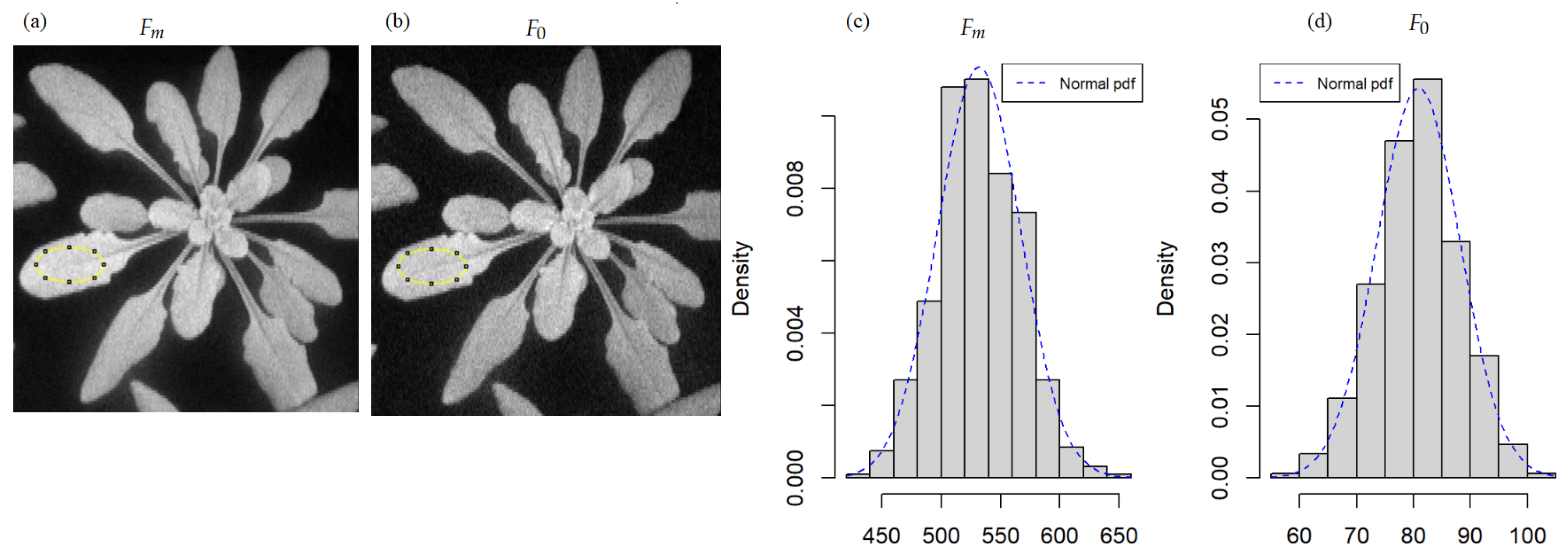
Example of chlorophyll fluorescence images of Arabidopsis thaliana inoculated by a bacteria, at day 2, pot 19, a healthy pot (inoculated with water): (a) maximum fluorescence and (b) minimum fluorescence. The histograms (c,d) are the associated frequency distribution of pixel counts inside the region of interest drawn in a solid yellow line in (a,b), respectively. The dashed blue line in the histograms is the fit with a normal probability density function (pdf).
Figure 1.
Example of chlorophyll fluorescence images of Arabidopsis thaliana inoculated by a bacteria, at day 2, pot 19, a healthy pot (inoculated with water): (a) maximum fluorescence and (b) minimum fluorescence. The histograms (c,d) are the associated frequency distribution of pixel counts inside the region of interest drawn in a solid yellow line in (a,b), respectively. The dashed blue line in the histograms is the fit with a normal probability density function (pdf).
Figure 2.
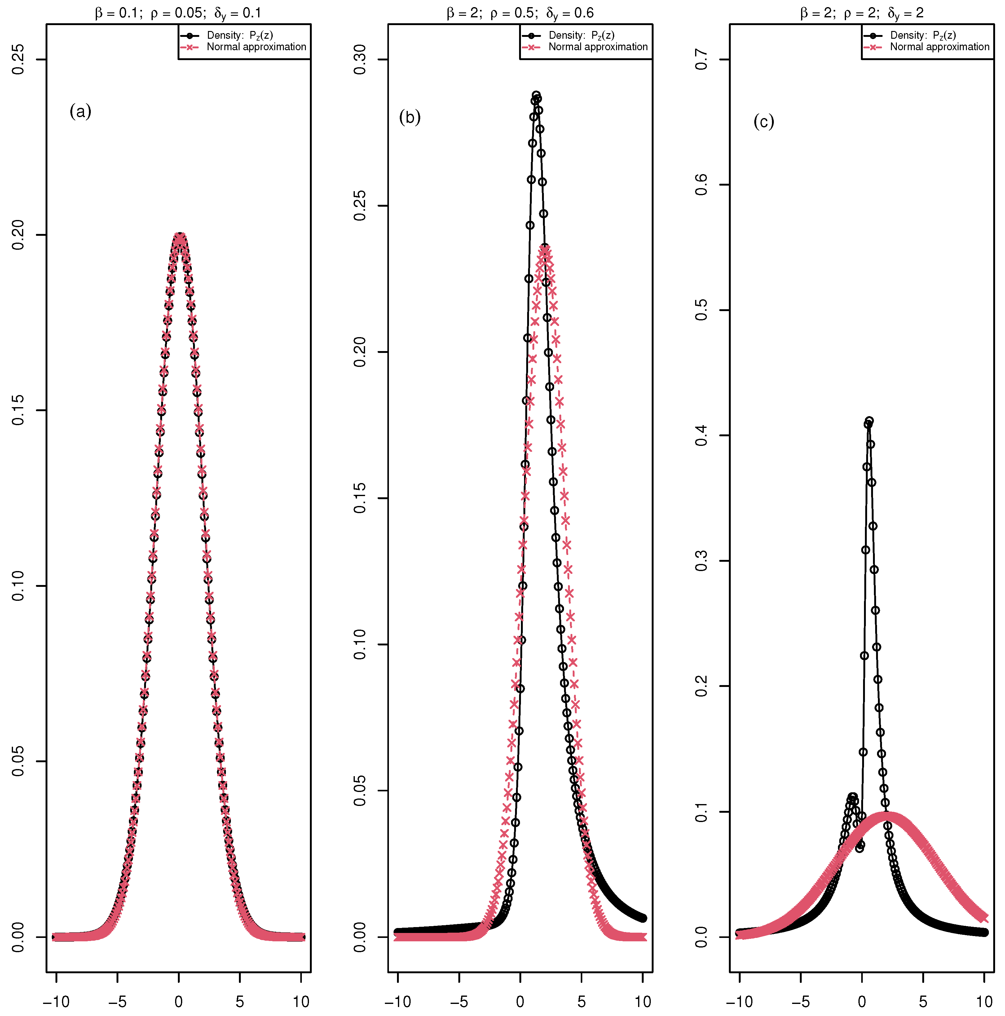
The black curve with circle points is the distribution of the ratio ( maximum fluorescence and , minimum fluorescence) for an increasing values of the parameters, , , and and the red curve with crossed points is the normal approximation of the distribution in each of these cases. (a) A case with perfect fit of the ratio density and the normal approximation; (b) a deviation from normal distribution; (c) a case where the ratio density is bimodal and the normal approximation is not appropriate.
Figure 2.
The black curve with circle points is the distribution of the ratio ( maximum fluorescence and , minimum fluorescence) for an increasing values of the parameters, , , and and the red curve with crossed points is the normal approximation of the distribution in each of these cases. (a) A case with perfect fit of the ratio density and the normal approximation; (b) a deviation from normal distribution; (c) a case where the ratio density is bimodal and the normal approximation is not appropriate.
Figure 3.
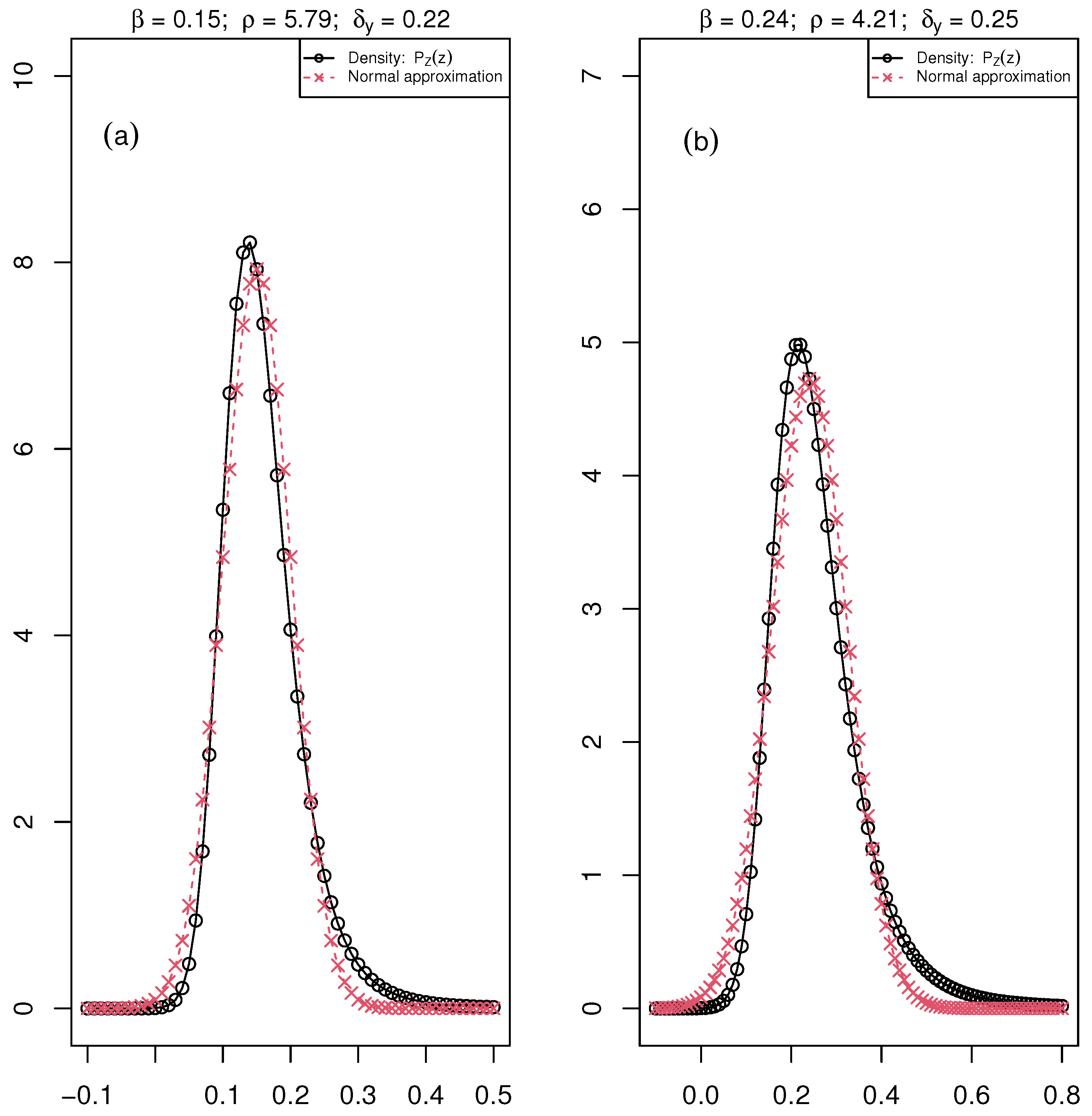
The distribution of the ratio ( maximum fluorescence and , minimum fluorescence) is the black curve with circle points, and the normal approximation is the red curve with crossed points. The parameters , , and of the distribution are associated with the mean value of these parameters over the six days of the acquisition of chlorophyll fluorescence images for (a) Healthy: , and and (b) Diseased: , and plants of the bacteria data set.
Figure 3.
The distribution of the ratio ( maximum fluorescence and , minimum fluorescence) is the black curve with circle points, and the normal approximation is the red curve with crossed points. The parameters , , and of the distribution are associated with the mean value of these parameters over the six days of the acquisition of chlorophyll fluorescence images for (a) Healthy: , and and (b) Diseased: , and plants of the bacteria data set.
Figure 4.
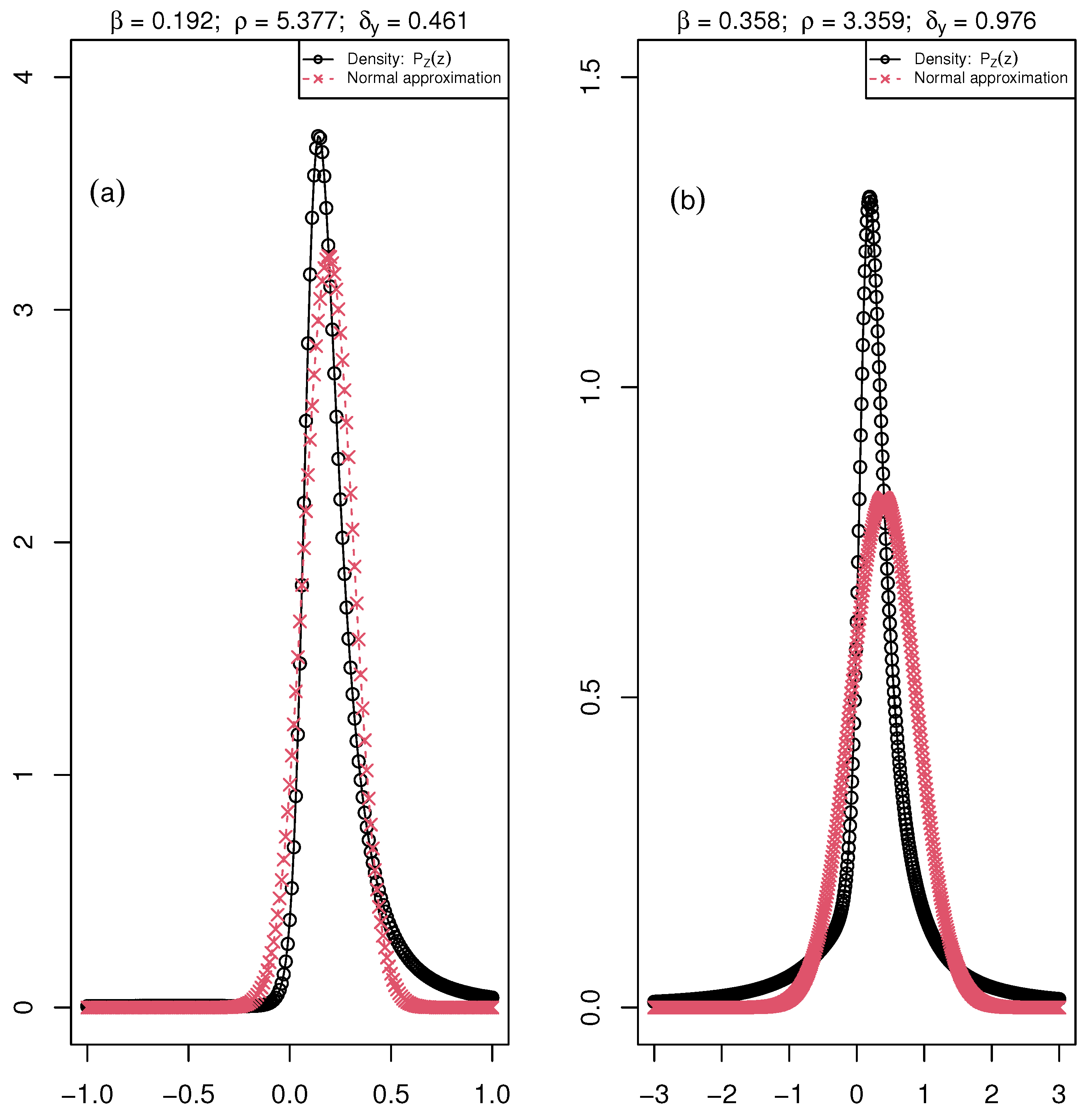
The distribution of the ratio ( maximum fluorescence and , minimum fluorescence) is the black curve with circle points, and the normal approximation is the red curve with crossed points. The parameters , , and of the distribution are associated with the mean value of these parameters over the six days of the acquisition of chlorophyll fluorescence images for (a) Healthy: , and and (b) Diseased: , and plants of the fungal pathogen data set.
Figure 4.
The distribution of the ratio ( maximum fluorescence and , minimum fluorescence) is the black curve with circle points, and the normal approximation is the red curve with crossed points. The parameters , , and of the distribution are associated with the mean value of these parameters over the six days of the acquisition of chlorophyll fluorescence images for (a) Healthy: , and and (b) Diseased: , and plants of the fungal pathogen data set.
Table 1.
Mean ± the standard deviation of four p-values associated with the D’Agostino test of normality in the limb of the Arabidopsis thaliana inoculated by a bacteria for maximum fluorescence and minimum fluorescence. D0, …, and D8 are the six days of the acquisition of chlorophyll fluorescence images.
| Time | | |
|---|
| Healthy | Diseased | Healthy | Diseased |
|---|
| D0 | 0.53 ± 0.33 | 0.55 ± 0.25 | 0.59 ± 0.34 | 0.60 ± 0.33 |
| D2 | 0.39 ± 0.25 | 0.59 ± 0.35 | 0.31 ± 0.25 | 0.57 ± 0.38 |
| D5 | 0.60 ± 0.38 | 0.45 ± 0.31 | 0.33 ± 0.19 | 0.31± 0.18 |
| D6 | 0.30 ± 0.22 | 0.46 ± 0.23 | 0.47± 0.33 | 0.44 ± 0.26 |
| D7 | 0.27 ± 0.10 | 0.24 ± 0.19 | 0.43 ± 0.31 | 0.44 ± 0.10 |
| D8 | 0.26 ± 0.16 | 0.25 ± 0.10 | 0.25 ± 0.14 | 0.11 ± 0.04 |
Table 2.
Mean , and standard deviation, , values on Healthy and Diseased tissues of chlorophyll fluorescence parameters (minimum fluorescence) and (maximum fluorescence) for images of plants inoculated with bacteria. D0, …, and D8 are the six days of the acquisition of chlorophyll fluorescence images.
| Time | | | | |
|---|
| Healthy | Diseased | Healthy | Diseased | Healthy | Diseased | Healthy | Diseased |
|---|
| D0 | 62.845 | 42.158 | 15.261 | 6.870 | 418.173 | 182.367 | 89.129 | 33.985 |
| D2 | 64.756 | 78.609 | 16.343 | 15.380 | 432.239 | 338.601 | 95.681 | 63.571 |
| D5 | 67.168 | 76.984 | 16.796 | 21.338 | 438.586 | 301.224 | 96.591 | 87.018 |
| D6 | 67.402 | 77.424 | 17.150 | 21.545 | 444.460 | 306.174 | 99.267 | 86.616 |
| D7 | 68.781 | 77.363 | 17.407 | 21.546 | 447.470 | 306.662 | 100.153 | 87.427 |
| D8 | 67.256 | 74.562 | 16.961 | 21.719 | 441.044 | 305.809 | 98.580 | 86.968 |
Table 3.
Mean , and standard deviation, , values on Healthy and Diseased tissues of chlorophyll fluorescence parameters (minimum fluorescence) and (maximum fluorescence) for the data set of plants infected with fungal pathogen data. 0 h, …, 96 h are the five times of the acquisition of chlorophyll fluorescence images.
| Time | | | | |
|---|
| Healthy | Diseased | Healthy | Diseased | Healthy | Diseased | Healthy | Diseased |
|---|
| 0 h | 142.747 | - | 31.056 | - | 810.626 | - | 192.474 | - |
| 24 h | 122.533 | 123.685 | 52.404 | 77.543 | 676.331 | 329.290 | 275.724 | 277.567 |
| 48 h | 105.450 | 82.616 | 56.436 | 66.731 | 537.056 | 222.493 | 295.606 | 203.232 |
| 72 h | 121.525 | 73.177 | 40.216 | 42.067 | 618.474 | 172.596 | 225.188 | 150.189 |
| 96 h | 103.579 | 43.691 | 50.808 | 41.099 | 526.299 | 103.953 | 274.768 | 133.111 |
Table 4.
The values of , and associated with the fluorescence data on Healthy and Diseased plants of the bacteria data set. D0, …, and D8 are the six days of the acquisition of chlorophyll fluorescence images.
Table 4.
The values of , and associated with the fluorescence data on Healthy and Diseased plants of the bacteria data set. D0, …, and D8 are the six days of the acquisition of chlorophyll fluorescence images.
| Time | | | |
|---|
| Healthy | Diseased | Healthy | Diseased | Healthy | Diseased |
|---|
| D0 | 0.150 | 0.231 | 5.840 | 4.947 | 0.213 | 0.186 |
| D2 | 0.150 | 0.232 | 5.855 | 4.133 | 0.221 | 0.188 |
| D5 | 0.153 | 0.256 | 5.751 | 4.078 | 0.220 | 0.289 |
| D6 | 0.152 | 0.253 | 5.788 | 4.020 | 0.223 | 0.283 |
| D7 | 0.154 | 0.252 | 5.753 | 4.058 | 0.224 | 0.285 |
| D8 | 0.152 | 0.244 | 5.812 | 4.004 | 0.224 | 0.284 |
Table 5.
The values of , and associated with the fluorescence data on Healthy and Diseased plants of the fungal pathogen data set. 0 h, …, 96 h are the five times of the acquisition of chlorophyll fluorescence images.
Table 5.
The values of , and associated with the fluorescence data on Healthy and Diseased plants of the fungal pathogen data set. 0 h, …, 96 h are the five times of the acquisition of chlorophyll fluorescence images.
| Time | | | |
|---|
| Healthy | Diseased | Healthy | Diseased | Healthy | Diseased |
|---|
| 0 h | 0.176 | | 6.198 | | 0.237 | |
| 24 h | 0.181 | 0.376 | 5.262 | 3.580 | 0.408 | 0.843 |
| 48 h | 0.196 | 0.371 | 5.238 | 3.046 | 0.550 | 0.913 |
| 72 h | 0.196 | 0.424 | 5.599 | 3.570 | 0.364 | 0.870 |
| 96 h | 0.197 | 0.420 | 5.408 | 3.239 | 0.522 | 1.280 |
Table 6.
Second-order fractional moment of distribution of the ratio for the healthy and diseased leaves of the bacteria data set. D0, …., and D8 are the six days of the acquisition of chlorophyll fluorescence images.
Table 6.
Second-order fractional moment of distribution of the ratio for the healthy and diseased leaves of the bacteria data set. D0, …., and D8 are the six days of the acquisition of chlorophyll fluorescence images.
| Plants | Time |
|---|
| D0 | D2 | D5 | D6 | D7 | D8 |
|---|
| Healthy | 0.608 | 0.608 | 0.604 | 0.606 | 0.603 | 0.605 |
| Diseased | 0.514 | 0.514 | 0.478 | 0.482 | 0.483 | 0.492 |
Table 7.
The mean value (
) and the associated standard deviation (
) of the second-order fractional moment of the Monte Carlo simulation for 10 and 80 sample sizes, with the first day of the experiment as a reference value, with the assumptions of Gaussian probability density function and the Gaussian approximation proposed in [
34] and with the two non-Gaussian estimators, Bayesian and EM.
| Method of Estimation | Plants, Sample Size (N) |
|---|
| Healthy, | Healthy, | Diseased, | Diseased, |
|---|
| | | |
| | | | | | | |
| Normal distribution | 0.591 | 0.037 | 0.613 | 0.009 | 0.524 | 0.016 | 0.523 | 0.007 |
| Normal approximation | 0.618 | 0.021 | 0.618 | 0.007 | 0.523 | 0.019 | 0.523 | 0.007 |
| Bayesian estimation | 0.608 | 0.022 | 0.608 | 0.008 | 0.515 | 0.020 | 0.514 | 0.007 |
| EM estimation | 0.612 | 0.017 | 0.608 | 0.008 | 0.516 | 0.021 | 0.513 | 0.008 |
Table 8.
Mean value of the relative error ( % ) for the five days of the experiment per method of estimation and per sample size, N, for Healthy and Diseased plants of the bacteria data set.
Table 8.
Mean value of the relative error ( % ) for the five days of the experiment per method of estimation and per sample size, N, for Healthy and Diseased plants of the bacteria data set.
| Method of Estimation | Plants, Sample Size (N) |
|---|
| Healthy, | Healthy, | Diseased, | Diseased, |
|---|
| | | |
| Normal distribution | 2 | 1 | 6 | 6 |
| Normal approximation | 2 | 2 | 6 | 6 |
| Bayesian estimation | 0 | 0 | 4 | 4 |
| EM estimation | 1 | 0 | 5 | 4 |
Table 9.
Fourth-order fractional moment of distribution of the ratio for the Healthy and Diseased plants of the fungal pathogen data set. 0 h, …, 96 h are the five times of the acquisition of chlorophyll fluorescence images.
Table 9.
Fourth-order fractional moment of distribution of the ratio for the Healthy and Diseased plants of the fungal pathogen data set. 0 h, …, 96 h are the five times of the acquisition of chlorophyll fluorescence images.
| Plants | Time |
|---|
| 0 h | 24 h | 48 h | 72 h | 96 h |
|---|
| Healthy | 0.349 | 0.335 | 0.304 | 0.322 | 0.306 |
| Diseased | - | 0.165 | 0.168 | 0.138 | 0.157 |
Table 10.
The mean value () and the associated standard deviation () of the fourth-order fractional moment of the Monte Carlo simulation with 24 h as a reference value.
Table 10.
The mean value () and the associated standard deviation () of the fourth-order fractional moment of the Monte Carlo simulation with 24 h as a reference value.
| Method of Estimation | Plants, Sample Size (N) |
|---|
| Healthy, | Healthy, | Diseased, | Diseased, |
|---|
| | | |
| | | | | | | |
| Normal distribution | 0.399 | 0.037 | 0.277 | 0.018 | 0.284 | 0.053 | 0.055 | 0.025 |
| Normal approximation | 0.370 | 0.035 | 0.369 | 0.012 | 0.231 | 0.055 | 0.231 | 0.019 |
| Bayesian estimation | 0.337 | 0.047 | 0.334 | 0.018 | 0.167 | 0.107 | 0.165 | 0.038 |
| EM estimation | 0.327 | 0.070 | 0.334 | 0.017 | 0.163 | 0.106 | 0.165 | 0.037 |
Table 11.
Mean value of the relative error (%) for the five times of the experiment per method of estimation and per number of observations for Healthy and Diseased plants of the fungal pathogen data set.
Table 11.
Mean value of the relative error (%) for the five times of the experiment per method of estimation and per number of observations for Healthy and Diseased plants of the fungal pathogen data set.
| Method of Estimation | Plants, Sample Size (N) |
|---|
| Healthy, | Healthy, | Diseased, | Diseased, |
|---|
| | | |
| Normal distribution | 26 | 12 | 82 | 65 |
| Normal approximation | 17 | 17 | 48 | 48 |
| Bayesian estimation | 7 | 6 | 7 | 7 |
| EM estimation | 5 | 6 | 6 | 7 |


