Use of Mohr Diagrams to Predict Fracturing in a Potential Geothermal Reservoir

Peacock, D.C.P.; Sanderson, David J.; Leiss, Bernd

doi:10.3390/geosciences11120501

Open AccessArticle

Use of Mohr Diagrams to Predict Fracturing in a Potential Geothermal Reservoir

by

D.C.P. Peacock

^1,2,*,

David J. Sanderson

³ and

Bernd Leiss

^1,2

¹

Geoscience Centre, Department of Structural Geology and Geodynamics, Georg-August-Universität Göttingen, Goldschmidtstraße 3, 37077 Göttingen, Germany

²

Universitätsenergie Göttingen GmbH, Hospitalstraße 3, 37073 Göttingen, Germany

³

Ocean and Earth Science, University of Southampton, National Oceanography Centre, Southampton SO14 3ZH, UK

^*

Author to whom correspondence should be addressed.

Geosciences 2021, 11(12), 501; https://doi.org/10.3390/geosciences11120501

Submission received: 24 September 2021 / Revised: 29 November 2021 / Accepted: 2 December 2021 / Published: 9 December 2021

(This article belongs to the Special Issue Enhanced Geothermal Systems and other Deep Geothermal Applications throughout Europe: The MEET Project)

Download

Browse Figures

Review Reports Versions Notes

Abstract

:

Inferences have to be made about likely structures and their effects on fluid flow in a geothermal reservoir at the pre-drilling stage. Simple mechanical modelling, using reasonable ranges of values for rock properties, stresses and fluid pressures, is used here to predict the range of possible structures that are likely to exist in the sub-surface and that may be generated during stimulation of a potential geothermal reservoir. In particular, Mohr diagrams are used to show under what fluid pressures and stresses different types and orientations of fractures are likely to be reactivated or generated. The approach enables the effects of parameters to be modelled individually, and for the types and orientations of fractures to be considered. This modelling is useful for helping geoscientists consider, model, and predict the ranges of mechanical properties of rock, stresses, fluid pressures, and the resultant fractures that are likely to occur in the sub-surface. Here, the modelling is applied to folded and thrusted greywackes and slates, which are planned to be developed as an Enhanced Geothermal System beneath Göttingen.

Keywords:

stress; fluid pressure; Mohr diagrams; fracturing; geothermal; greywackes; slates

1. Introduction

A study is being undertaken to predict the structures and fluid flow behaviour in the sub-surface as part of a proposed geothermal project at Göttingen in Germany [1,2,3]. The reservoir rocks are the Devonian and Carboniferous metasedimentary sequence thought to occur at a depth of ~1.5 km, beneath a cover of Permian and Mesozoic sedimentary rocks [4]. Göttingen is one of the sites within the European funded project Multidisciplinary and multi-context demonstration of EGS exploration and Exploitation Techniques and potentials (MEET) to develop enhanced geothermal systems (EGS) across Europe (e.g., [5,6,7]). The Triassic Bunter Sandstone is also being considered as a potential medium-deep geothermal reservoir (i.e., at depths between about 200 m and 1000 m; e.g., [8]), including heat storage options [2], and this is also discussed here.

Only two wells have yet penetrated the metasedimentary rocks in the Göttingen area, these not extending far below the base Zechstein, and so limited well data are available. Additionally, the limited seismic data available show poor resolution beneath the Zechstein salt (e.g., [9,10]). Two seismic lines were shot in 2015, these being 10 km and 11 km long and to about 5 km deep. These seismic lines allow interpretation of the post-Carboniferous sedimentary rocks in the north-south striking Leinetal Graben [3], but do not enable reliable interpretation of the sub-Zechstein rocks. The metasedimentary rocks exposed in the Harz Mountains, ~40 km NE of Göttingen, are being used to predict the rocks and structures that may occur in the sub-surface at Göttingen, and to gain data input for discrete fracture network (DFN) modelling. Exposures of the Bunter Sandstone occur in the area around Göttingen (e.g., [11,12,13]).

There are significant uncertainties involved in evaluating the characteristics and mechanical properties of the rocks beneath Göttingen. Although field analogues indicate many different types of natural fractures occur (faults, veins, joints, etc.), their intensity, geometry, topology and spatial variation in the sub-surface are unknown. Many of the fractures, especially the joints, may not exist at reservoir depths (e.g., [14,15]). The proposed EGS project would involve stimulation of intensely-deformed Upper Palaeozoic rocks, and there are significant uncertainties involved in predicting the hydraulic fracturing of such anisotropic and pre-fractured rocks (e.g., [16]).

Because there is limited knowledge of the reservoir rocks in the sub-surface, including such parameters as fracture types, orientations, apertures, and connectivity, there is need for an early-stage (pre-drilling) assessment that will enable reasonable predictions to be made about natural and induced fractures in the sub-surface. Here, we use simple modelling and reasonable values of stress states, fluid pressures and rock failure criteria to make predictions about the conditions under which rocks will fracture.

The aim of this paper is to develop a simple workflow in which we assess the likely stress states, fluid pressures, and failure conditions in the sub-surface. We then use Mohr diagrams (Figure 1; e.g., [17,18]) to make predictions of the behaviour of rocks and fluids within potential reservoir rocks. The approach uses information about rock types and structures obtained from exposed analogues and rock deformation tests to predict the effects of changes in effective stresses on natural and induced fractures. In the absence of information on the geometry and topology of the fracture networks and on the conductivity of the fractures, this represents an early-stage approach and a necessary prerequisite to more detailed analysis of the contribution of fractures to fluid flow, such as through the use of DFN modelling (e.g., [19]).

Although the approach is simple, it provides understanding of the relationships between key factors controlling rock behaviour. It helps us identify uncertainties and their possible effects. It can also be considered as a “dynamic” analysis for fracturing, because it can be used to predict the reactivation and generation of fractures as fluid pressures and stresses change. Here, reactivation is used to mean renewed shear and/or opening displacement on a pre-existing fracture.

The methods presented here have general applicability to making predictions about fractures in the sub-surface, but here we focus on several key questions about the proposed geothermal reservoir at Göttingen:

Which lithologies are most likely to fracture?
What stresses and fluid pressures are needed for the reactivation of pre-existing fractures or the development of new fractures?
Which orientations and types of fractures are most likely to be reactivated?
Will reactivated or new fractures show shear or extension?
What effects do heterogeneities (veins, joints, cleavage, bedding planes) have, and what are the different mechanical significances of veins vs. joints?
What are the effects of Late Cretaceous and Tertiary exhumation and what amount of exhumation is needed to create joints?

2. Predictions about the Pre-Permian Geology beneath Göttingen

In the absence of well data or high-quality seismic data for the sub-Zechstein rocks, the rocks beneath the Permian Zechstein evaporites at Göttingen are predicted to be Devonian quartzitic sandstones and slates, and Carboniferous greywackes and slates (mainly Culm flysch deposits). Such rocks are exposed in the western Harz Mountains ~40 km to the NE, in the Oberharz Anticline and the Culm Fold Zone, which belong to the par-autochthonous domain of the Harz Mountains (e.g., [3,20]) and in the Rhenish Massif ~70 km to the SW (e.g., [21,22,23]). The fractures visible in these exposures include veins and joints [24], with cleavage being well-developed in the slates [25]. Small thrusts that appear to have displacements of up to a few metres are exposed [26], but larger thrusts are not well-exposed. The north-eastern boundary the Harz Mountains is marked by the Harznordrand Fault, which was active during the Late Cretaceous and Tertiary [27]. NW-SE striking Mesozoic normal and oblique-slip faults occur in the Harz Mountains, some of which contained economic Pb-Zn and Ba-F deposits [28].

Figure 1. (a) Generalised Mohr diagram of shear stress (τ) against normal effective stress (σ′_N) showing failure envelopes. Continuous line (“Cohesional”) = Mohr failure envelope for intact rock, with tensile strength (T = 2 MPa), cohesion (S₀ = 4 MPa) and coefficient of internal friction (μ = 0.75). Dotted (parabolic) line (“Griffith”) = Griffith criterion. Dashed line (“Cohesionless”) = cohesionless failure (μ = 0.75) typical of slip on faults. Three stress states are shown, representing stable (➊), shear failure on cohesionless fractures (➋) and extension fracturing (➌). (b) Mohr diagram showing the fields in which extension (➊), hybrid (➋) and shear (➌) fractures occur [29].

Table 1 shows features of these “basement” rocks that are likely to be important for geothermal energy. These predictions are expressed in terms of seven parameters that we consider important in describing a geothermal reservoir: lithology and inferred rheological behaviour, fluid type, stresses, fluid pressure, temperature, strains and existing structures, and geological history (cf. [30]).

More information is available about the Bunter Sandstone, which is exposed in the Göttingen area (e.g., [11,12]). Fractures exposed include normal faults [31], strike-slip faults [32], veins [33], sedimentary dykes [34], and joints [35]. There is limited well data, which suggests that the Bunter Sandstone has been affected by halokinesis of the Zechstein evaporites [1,36,37].

Table 1. Predictions about the geology of the potential geothermal reservoirs at Göttingen. See, for example, [38] for full information about deformation of the Bunter Sandstone in the Leinetal Graben. See [20,39] for further information about the geology of the Devonian and Carboniferous rocks of the Harz Mountains.

Factor	Meaning	Significance	Bunter Sandstone	Variscan rocks
Lithology	Rock types, their porosities and mechanical behaviour	Controls the thermo-mechanical behaviour of the rock. Mechanical behaviour can change significantly through time, especially as deformation occurs	Triassic sandstone (see Table 2 for mechanical properties)	Devonian and Carboniferous greywackes and slates (see Table 2 for mechanical properties)
Fluid type	The chemistry and phase (liquid or gas) of the palaeo- and present-day fluid(s)	Controls the fluid pressure gradient and mineralisation events	Present-day: water (possibly brine)	Present-day: water, probably saline because of the overlying Zechstein. No information on gas content. During the Variscan: mineralising fluids and fluidised sediments
Stress	Magnitudes and orientations of the applied stresses, including the vertical stress (overburden) and horizontal stresses. Horizontal stresses are related to the geostatic stress ratio, applied tectonic stresses and to internal stresses (e.g., related to temperature changes)	Along with fluid pressure, controls the effective stresses, which control the deformation	The vertical stress can be calculated using the mean density of the overburden, but the magnitudes and orientations of the horizontal stresses are uncertain	The vertical stress can be calculated using the mean density of the overburden, but the magnitudes and orientations of the horizontal stresses are uncertain
Fluid pressure	Palaeo- and present-day fluid pressures	Along with the stresses, controls the effective stresses, which control the deformation	Presently probably hydrostatic	The Zechstein evaporites may allow present-day overpressure. Veins, breccias and possible remobilised sediments indicate phases of overpressure during the Variscan Orogeny
Temperature	Palaeo- and present-day temperatures	Influences the style of deformation, with present-day temperature controlling commercial viability	Depends on the geothermal gradient	Depends on the geothermal gradient, but likely to be reduced because of the overlying salt. Possibly elevated by Tertiary igneous activity
Strain	The amount of strain and the existing structures	Influences fluid flow in the sub-surface and present-day mechanical behaviour of the rocks	Controlled by Tertiary rifting. Likely to be influenced by salt tectonics and possibly by Tertiary igneous activity. Steeply-dipping joints and some normal faults are likely to occur	Dominated by: (1) Variscan Orogeny, with folds, thrusts and veins; (2) Late Cretaceous and Tertiary rifting and/or uplift, with normal faults and joints developing
History	The relative and absolute timing of deformation (including mineralisation) events and structures	Controls the types of fractures (faults, veins, joints, etc.) and therefore their effects on fluid flow in the sub-surface	(1) Triassic sedimentation during Mesozoic basin development. (2) Cretaceous and Tertiary regional uplift. (3) Tertiary rifting (Leinetal Graben) and volcanism	(1) Sedimentation during the Devonian and Carboniferous. (2) Variscan Orogeny. (3) Permian and Mesozoic sedimentation and basin development. (4) Cretaceous and Tertiary regional uplift. (5) Tertiary rifting and volcanism

3. Model Set-Up

A Microsoft Excel spreadsheet has been created to make the necessary calculations and to plot Mohr diagrams (e.g., Figure 2). For simplicity, we keep the Mohr diagram analysis two-dimensional, considering just the vertical stress and the horizontal stress in one direction. This approach is taken both because it simplifies the analysis and because the orientations and magnitudes of the horizontal stresses are presently unconstrained. We start with a reference state where the horizontal strains are zero, which is the uniaxial strain condition (e.g., [58]) and the horizontal effective stress (σ′_H) is given by:

σ′_H = k₀ σ′_V

(1)

where k₀ is the geostatic stress ratio [59] or coefficient of lateral earth pressure [60]. The geostatic stress ratio is the ratio of the horizontal effective stress to the vertical effective stress (i.e., k₀ = σ′_H/σ′_V). For an isotropic elastic material:

k₀ = ν/(1 − ν)

(2)

where ν is Poisson’s ratio, which is generally in the range 0 to 0.5 (where 0.5 is incompressible). For most water-saturated rocks, is in the range 0.15 < ν < 0.4 (e.g., [61]).

We consider the vertical stress to result from the weight of the overlying material and the horizontal stresses to result from the combined effects of the geostatic stress ratio and the applied tectonic stresses. We start the analysis with a base-case, in which fluid pressure is hydrostatic and there are no applied tectonic stresses. We then consider how changes in fluid pressure and/or apply tensile or compressional horizontal (“tectonic”) stresses might lead to fracturing.

3.1. Mohr Diagrams, Stresses and Failure Envelopes

Mohr diagrams are commonly used to show the relationships between stresses, fluid pressure, and fractures (Figure 1a; e.g., [62]). They provide a convenient graphic representation of the effective stress states and of failure (e.g., [17]). Normal stress (σ_N) is plotted on the x-axis and shear stress (τ) on the y-axis, with the principal axes of stress (σ₁ = maximum compressive stress, σ₂ = intermediate compressive stress, σ₃ = minimum compressive stress) or principal axes of effective stress (σ′₁ = maximum effective compressive stress, etc., where σ′ = σ − B.P_F, where P_F = fluid pressure and B is Biot’s constant, which we will assume to be approximately 1). Since the magnitudes and orientations of the horizontal stresses are currently unknown, we consider stress in 2D, with σ₂ being ignored (e.g., [63]). We assume an Andersonian stress regime with one principal stress vertical (the overburden stress, σ_V) and the other horizontal stress (σ_h) [64]. In the base case models used here, the starting point is that there are no applied tectonic stresses, so σ_V = σ₁, and σ_h = σ₃ (Figure 2).

Figure 2. Base case Mohr diagrams, with Mohr circles for end-member geostatic stress ratios (k₀) shown (see Table 3 for parameters used). Representative dips of structures are shown to illustrate which of these structures might be reactivated under different stress conditions. (a) The Bunter Sandstone. (b) Devonian and Carboniferous greywackes at a depth of 2 km. (c) Devonian and Carboniferous slates at a depth of 2 km. (d) Devonian and Carboniferous greywackes at a depth of 4.5 km. (e) Devonian and Carboniferous slates at a depth of 4.5 km.

Any 2D state of effective stress can be represented by a circle that intersects the x-axis at σ′₁ and σ′₃, with the centre of the circle representing the mean stress (σ′_Mean = (σ′₁ + σ′₃)/2). Mohr diagrams are useful for illustrating the conditions under which fracturing may occur in a particular rock under specific conditions (i.e., the failure envelope), but only if the effective stresses are plotted.

Fracturing is classically attributed to conditions where the effective stress components exceed some critical value, usually termed the strength, which is thought to be a property of the material (e.g., [65]). Tensile failure occurs if:

σ′₃ ≤ T

(3)

where T is the tensile strength. Compressive stresses are positive. Shear failure occurs if:

τ ≥ S₀ + μ σ_N

(4)

where µ is the coefficient of (internal) friction and S₀ is the cohesion. These conditions are usually linked to produce a failure envelope (e.g., [66,67]), as in Figure 1a.

The composite failure criteria used in this work (e.g., Figure 1 and Figure 2) combine a linear, Mohr–Coulomb envelope for shear fracture under compressive effective stresses, with a parabolic, plane Griffith envelope for tensile/hybrid fractures under tensile stress conditions. The two envelopes join at the τ-axis (σ′ = 0), where there is a discontinuity in the slopes of the failure envelopes. Continuity in the slope could be achieved by using the methods outlined in [68]. This type of composite failure envelope is consistent with a modification of the Griffith theory to account for closure and frictional behaviour under compression [69,70].

Following [71], the plane Griffith failure envelope in Mohr space (τ, σ′) is given by:

τ ² = 4 T (σ′ + T)

(5)

and the Mohr–Coulomb envelope by:

τ = S₀ + μ σ′

(6)

where T = Tensile strength, S₀ = cohesion, and μ = coefficient of internal friction. Putting σ′ = 0 in both Equations (5) and (6) gives:

τ = S₀ = 2T

(7)

Hence, the cohesion would be simply twice the tensile strength. The unconfined compressive strength (C₀), is a widely measured parameter representing the stress required for failure when σ_3′ = 0 which for Mohr–Coulomb failure is given by:

C₀ = 2S₀ [(μ² +1)^1/2 + μ]

(8)

Substituting Equation (7) in Equation (8) gives:

C₀ = 4T [(μ² +1)^1/2 + μ]

(9)

Using a value of μ ≈ 1, gives the following approximations for rocks: (1) S₀ ≈ 0.2 C₀; (2) T ≈ 0.5 S₀; so (3) T ≈ 0.1 C₀ [71]. Sedimentary rocks typically show an exponential increase in C₀ with decreasing porosity [72].

We assume a lower bound to likely failure envelopes is given by the failure envelope shown by the “Cohesionless” line in Figure 1a, which is typical of slip on pre-existing cohesionless fractures (e.g., joints) (e.g., [73]). Such failure envelopes typically have coefficients of friction of 0.6 to 0.9 (average 0.75; e.g., [74]).

In Figure 1a, the effective stress state shown by Mohr circle ➊ is typical of a rock at depth of ~2 km, with the maximum compressive stress being vertical (σ_V) and caused by the weight of the overlying material. The rock is under a hydrostatic fluid pressure (where P_F/σ_V = ~0.4, based on the assumption that P_F ~ 20 MPa and σ_V~50 MPa at 2 km) and a tectonic stress (−2 MPa, as may occur during regional extension). Note that this is in the stable region, but within ~5 MPa of the failure envelope for rocks with cohesionless fractures. Figure 1a shows stress states that are stable (➊), that would cause slip on a suitably orientated pre-existing cohesionless fractures (➋), and that would create tensile failure of the intact rock (➌).

In this paper, we use Mohr diagrams to illustrate the conditions under which a rock can go from a stable stress system (i.e., no active fracturing occurs) to an unstable stress system (i.e., fracturing occurs). The change from stable to unstable condition depends upon:

The rock properties used to define the failure envelope are the tensile strength (T), uniaxial compressive strength (UCS), cohesion (S₀), and coefficient of internal friction (μ) [75];
The stress state (σ), which is defined in terms of principal stresses, mean stress and differential stress [17]. Stresses are in turn controlled by factors, such as depth of burial (overburden), tectonic (horizontal) stresses, and other changes in the physical state of the material, such as expansion or contraction caused by temperature and volume change (e.g., [76]). Changes in stresses that lead to fracturing can either be by increasing [77] or reducing the [78] the applied compressive stresses;
In the upper crust, fluid pressure in the pores and cracks combines with the applied stresses to produce an effective stress, where σ′ = σ − P_F (e.g., [79,80,81]). In the absence of specific information, we use a Biot coefficient (B) of 1, where σ′ = σ − B.P_F [82]. Changes in fluid pressure that can lead to fracturing can either be an increase in fluid pressure (e.g., [83]) or a reduction in fluid pressure, which can cause pore collapse (e.g., [84,85]). Pore collapse is not considered further in this paper.

The type and orientation of fractures developed can be predicted from the relationship between the Mohr circle for effective stress and the failure envelope (Figure 1b). Extension fractures typically develop perpendicular to the direction of σ′₃ if σ′₃ touches the failure envelope on the τ = 0 axis (Figure 1b➊), which generally requires a relatively low differential effective stress (σ′_Diff = σ′₁ − σ′₃). Shear fractures are predicted to develop if the Mohr circle touches the failure envelope in the compressive field (Figure 1b➌), this typically requiring a relatively high σ′_Diff. Hybrid fractures develop by synchronous extension and shear (e.g., [29]), and occur if the Mohr circle touches curved part of the failure envelope within the tensile field of the Mohr diagram (Figure 1b➋).

3.2. Input Data, Assumptions, and Uncertainties

Table 2 shows values from the literature for various rock mechanical parameters for the Bunter Sandstone, greywackes, and slates derived from triaxial tests. Table 2 also gives definitions and the significance of each parameter. Triaxial tests typically use intact hand specimen sized rock samples with no pre-existing fractures visible. As such, these values almost certainly over-estimate the strengths of the larger rock masses in the sub-surface, which generally have pre-existing fractures (e.g., [86]), and should be considered as upper-limit values of rock strength. We, therefore, use lower values for rock strength as inputs into the models (Table 3). The failure envelope (e.g., Figure 2) for each rock type is controlled by the tensile strength (T), cohesion (S₀) and coefficient of internal friction (μ = tan φ, where φ = angle of internal friction) (Equations (3) and (4)). The most widely available rock strength parameter is the uniaxial compressive strength (UCS or C₀), determined directly from triaxial tests or estimated from geophysical log data [72,73].

Note that the values presented in Table 3 are generally within the ranges of values for Devonian and Carboniferous greywackes and slates in the Harz Mountains and Belgium presented by [87]. Exceptions are the porosity (greywackes, mean value = 2.42%, range 0.04 to 7.35%, n = 88; slates, mean value = 2.21%, range 0.17 to 5.51%, n = 20), and the cohesion of the greywackes (mean value = 26.57 MPa, range 10.5 to 45.9 MPa, n = 5).

The Mohr circle for effective stress is controlled by the applied stresses and the fluid pressure. The vertical stress can be calculated from the densities of the overlying rocks (e.g., [73,88]). The magnitudes and orientations of these horizontal stresses are much harder to calculate (e.g., from well data; [89]) or predict (e.g., from tectonic stress tensors; [90]). Similarly, pore fluid pressure in rocks in the sub-surface is difficult to predict without well data. For example, [91] use sediment consolidation experiments and numerical models to predict fluid pressures.

In the absence of appropriate sub-surface data, the magnitudes of the horizontal stresses are considered in terms of the geostatic stress ratio of the rock (e.g., [92]). The pore pressures are discussed in terms of the hydrostatic pressure and any assumed overpressure.

The modelling presented here makes several assumptions. These assumptions are made to act as a starting point, to simplify the analysis and because of the various uncertainties:

An Andersonian stress system is assumed, i.e., with one of the principal axes of stress being vertical and the other two being horizontal [64];
The analysis is carried out in two-dimensions, considering just vertical stress and horizontal stress. This simplifies the analysis and is, we argue, justified at the pre-drilling stage of analysis because of the magnitudes and orientations of the horizontal stresses are currently unknown. Hydrofracture data from three wells in the region suggest a thrust regime with a maximum horizontal stress orientated ~WNW-ESE [93];
The vertical stress is produced by the weight of overburden;
The fluids are hydrostatically pressured;
The failure parameters used in the modelling (Table 3) are assumed to be representative of the rock properties in the sub-surface.

3.3. Base Case Models

We start with base case models (Figure 2) to derive threshold conditions for the reactivation of fractures or the generation of new fractures. These base cases use the uniaxial strain condition (e.g., [58]), with no applied tectonic stresses. The fluids in pore spaces and open fractures are hydrostatically pressured, with the water table being at the ground surface. In such circumstances, the vertical effective stress creates a horizontal effective stress that is given by the geostatic stress ratio (Figure 2), with the input parameters used shown in Table 3. The base case models are used as a starting point for experiments in which fluid pressure is increased (as would occur either by natural overpressure or by hydraulic stimulation), and the horizontal (tectonic) stress either decreased or increased, until the model predicts either the reactivation of existing cohesionless fractures (hydraulic stimulation) or the generation of new fractures.

For most rocks, T << 100 MPa, with poorly-consolidated sediments having T → 0, whereas for shear failure 0.5 < μ < 1.5 (generally) and 0 < S₀ < 50 MPa. In this paper, we use ranges of T, S₀, and μ that are appropriate for the rocks being considered.

An important point illustrated by Figure 2 is that, at typical K₀ values (0.3–0.5), the stress state is stable and no fracturing would be expected. This means that low K₀ values are needed to allow failure in the base case model, which simulates simple burial, with hydrostatic fluid pressure and no applied tectonic stresses. Any failure would largely be by shearing of pre-existing fractures, which may occur in the Devonian and Carboniferous rocks that are considered to occur beneath Göttingen.

3.4. A Range of Stress States for Fracturing

We consider a range of states of effective stress, seven of which are shown in Figure 3, together with their effect on fracturing. Note that the discussion is of changes in effective stresses, which can be caused by changes in applied stresses and/or fluid pressure. These states of stress have been modelled for the Bunter Sandstone and the Devonian and Carboniferous greywackes and slates by increasing the fluid pressure and by applying “tectonic” stresses to the base case models.

4. Effects of Key Parameters

A definition and the significance of each of the input parameters, along with representative values, are given in Table 2. For a given overburden stress, higher geostatic stress ratios produce larger horizontal stress and, hence, lower differential stress (Figure 2). The effects of other key parameters are illustrated in Figure 4. The position and shape of the failure envelope is controlled by the tensile strength, cohesion, and coefficient of internal friction of the rock (Figure 4a). Vertical, and therefore horizontal, stress increases with depth as the overburden increases (Figure 4b). High values of compressional tectonic stress can cause the horizontal stress to exceed the vertical stress, tending to lead to shear failure, while tensile tectonic stress will increase the differential stress and may lead to the development of extension fractures (Figure 4c). Increases in fluid pressure move the Mohr circle for effective stress to the left, towards more tensile parts of the Mohr diagram (Figure 4d). Note, however, that a change in fluid pressure will cause a change in differential stress that is proportional to the geostatic stress ratio, and it is a common mistake to show a constant differential stress with changing fluid pressure (e.g., [94,95]). The base cases are close to cohesionless failure if lower K₀ values are used, which implies that fracturing will generally require some tectonic stress and/or overpressure, especially to initiate the development of new fractures.

Figure 3. A range of effective stress states for fracturing illustrated using Mohr diagrams and sketch cross-sections with cohesive fractures (e.g., veins) and non-cohesive fractures (e.g., joints) dipping at 90°, 45°, and 0°. σ_V = vertical stress, σ_h = horizontal stress. (a) Stable stress state, in which the effective stresses are insufficient to reactivate existing fractures or create new fractures. (b) Reduced effective stresses, such that favourably-orientated pre-existing cohesionless fractures can be reactivated as shear fractures. (c) Reduced effective stresses, such that favourably-orientated pre-existing cohesionless fractures can be reactivated as shear fractures. (d) Reduced effective stresses, such that new extension fractures are created perpendicular to the least effective stress. (e) Reduced effective stresses (e.g., as fluid pressure increases), such that new extension fractures with any orientation can be created. (f) Increased effective stresses, such that favourably-orientated pre-existing cohesionless fractures are reactivated as shear fractures. (g) Increased effective stresses, such that new shear fractures are generated.

The Mohr diagrams presented in Figure 2, Figure 3 and Figure 4 show two types of failure envelope. The “Cohesionless” lines on the Mohr diagrams are typical of slip on pre-existing unfilled fractures (e.g., joints; Figure 5a), while the “Cohesional” lines represent the behaviour of intact rock or fractures that are filled by cohesive material (e.g., veins or faults with cohesive gouge; Figure 5b). These different failure envelopes illustrate the different mechanical behaviours of such cohesionless fractures as joints and such cohesional fractures as fully-filled veins and faults with clay gouge, highlighting the importance of distinguishing between different fracture types when using a field analogue for a geothermal reservoir.

5. Potential for Reactivating and Generating Fractures

Results of the models can be expressed in terms of the critical values of fluid pressure or horizontal (tectonic) stresses needed to reactivate existing cohesionless fractures, or to generate new fractures (Table 4). Note that these are simply the results of the model, which is based on poorly constrained parameters and should only be taken as suggestions of what may occur under the conditions stated.

5.1. Bunter Sandstone

Critical values predicted by the modelling for the Bunter Sandstone at a depth of 1 km are presented in Table 4, from which the following predictions can be made. (1) Favourably-orientated cohesionless fractures in the Bunter Sandstone may be critically stressed without fluid overpressure or applied tectonic stresses (i.e., the base-case model) if the geostatic stress ratio is low (e.g., 0.2). (2) Shear may therefore occur on favourably-orientated cohesionless fractures (e.g., joints) if the fluid is hydrostatically pressured (i.e., fluid pressure ~10 MPa; e.g., Figure 3b) for a geostatic stress ratio ~0.2, but a fluid pressure of about 24 MPa would be needed to reactivate cohesionless fractures if the geostatic stress ratio is ~0.54. (3) Gently-dipping extension fractures would start to develop at fluid pressures of about 30 MPa. (4) Steeply-dipping extension fractures will develop if there is a tensile tectonic stress of about 8.2 to 13.5 MPa (e.g., Figure 3d). (5) Extension fractures may develop in all directions if the fluid pressure is about 34 to 54 MPa (e.g., Figure 3e). (6) Favourably-orientated cohesionless fractures may be reactivated in shear (normal faulting) in the greywackes if there is a tensile tectonic stress of 0 to 3.7 MPa (e.g., Figure 3b). (7) Favourably-orientated cohesionless fractures may be reactivated as thrusts if there is a compressive tectonic stress of 43 to 48 MPa (e.g., Figure 3f). (8) New thrusts will develop if there is a compressive tectonic stress of about 90 to 95 MPa (e.g., Figure 3g).

Figure 5. Examples of fractures in Carboniferous greywackes, cherts and slates in the Harz Mountains. (a) Joints (cohesionless) in thinly-bedded greywackes and slates at Okerstausee, Niedersachsen. (b) Example of cohesional fractures at Lautenthal, Niedersachsen. Clay has been injected along faults with centimetre-scale displacements, related to block rotation in a chert bed accommodated by thickness variations in a slate layer.

Table 4. Results of the modelling for the Bunter Sandstone and the Lower Palaeozoic greywackes and slates, showing the calculated critical values. Values specific to a modelled depth of 2 km are shown in bold, and values specific to a modelled depth of 4.5 km are shown in italics. * Shear or hybrid fractures, rather than extension fractures, may develop in the slates under these conditions.

	Bunter Sandstone K₀ = 0.19	Bunter Sandstone K₀ = 0.54	Greywacke K₀ = 0.125	Greywacke K₀ = ratio = 0.41	Slate K₀ = 0.283	Slate K₀ = 0.41	Units	Notes
Fluid pressure, cohesionless	9.81	24	19.62 44.15	50 115	51 115	51 115	MPa	Shear on favourably-orientated cohesionless fractures
Fluid pressure, gently-dipping cohesional	29.5	30	72 138	72 138	68 134	68 134	MPa	Gently-dipping extension fracture develop
Fluid pressure, all orientations of extension fractures	54	34.4	210 278	100 168	105 172	90 155	MPa	Steep extension fractures develop
a. Base case	Unstable	Stable	Unstable Unstable	Stable	Stable	Stable	MPa	Stable stress state for higher K₀
b. Decreased tectonic stress, reactivation starts	0	−3.7	0 0	−7.5 −17	−2 −5	−6.5 −14	MPa	Shear on favourably-orientated cohensionless fractures
c. Decreased tectonic stress, many fractures reactivated	−5	−8	−10 −20	−20 −30	−10 −22	−14 −31	MPa	Shear on a cohesionless fractures with a wide range of orientations
d. Reduced tectonic stress, extension fractures develop	−8.2	−13.5	−24 −29	−33 −50	−24 −33 *	−28.5 −43 *	MPa	Extension fractures develop perpendicular to least compressive stress
e. Reduced tectonic stress, extension fractures in all orientations	N/A	N/A	N/A N/A	N/A N/A	N/A N/A	N/A N/A	MPa	Requires increase in fluid pressure
f. Increased tectonic stress, some reactivation of cohesionless	48	43	0 (normal) 180 (thrusts) 0 (normal) 400 (thrusts)	170 370	145 320	140 315	MPa	Reactivation of cohesionless fractures in shear
g. Increased tectonic stress, new shear fractures can develop	95	90	370 590	360 580	275 450	270 440	MPa	Creation of new shear fractures

5.2. Devonian and Carboniferous Greywackes and Slates

Critical values predicted by the modelling for the Devonian and Carboniferous greywackes and slates at depths of 2 km and 4.5 km are presented in Table 4. These depths are used because they represent the proposed depths for an initial research well and an exploitation well, respectively. The results of the modelling enable the following predictions to be made.

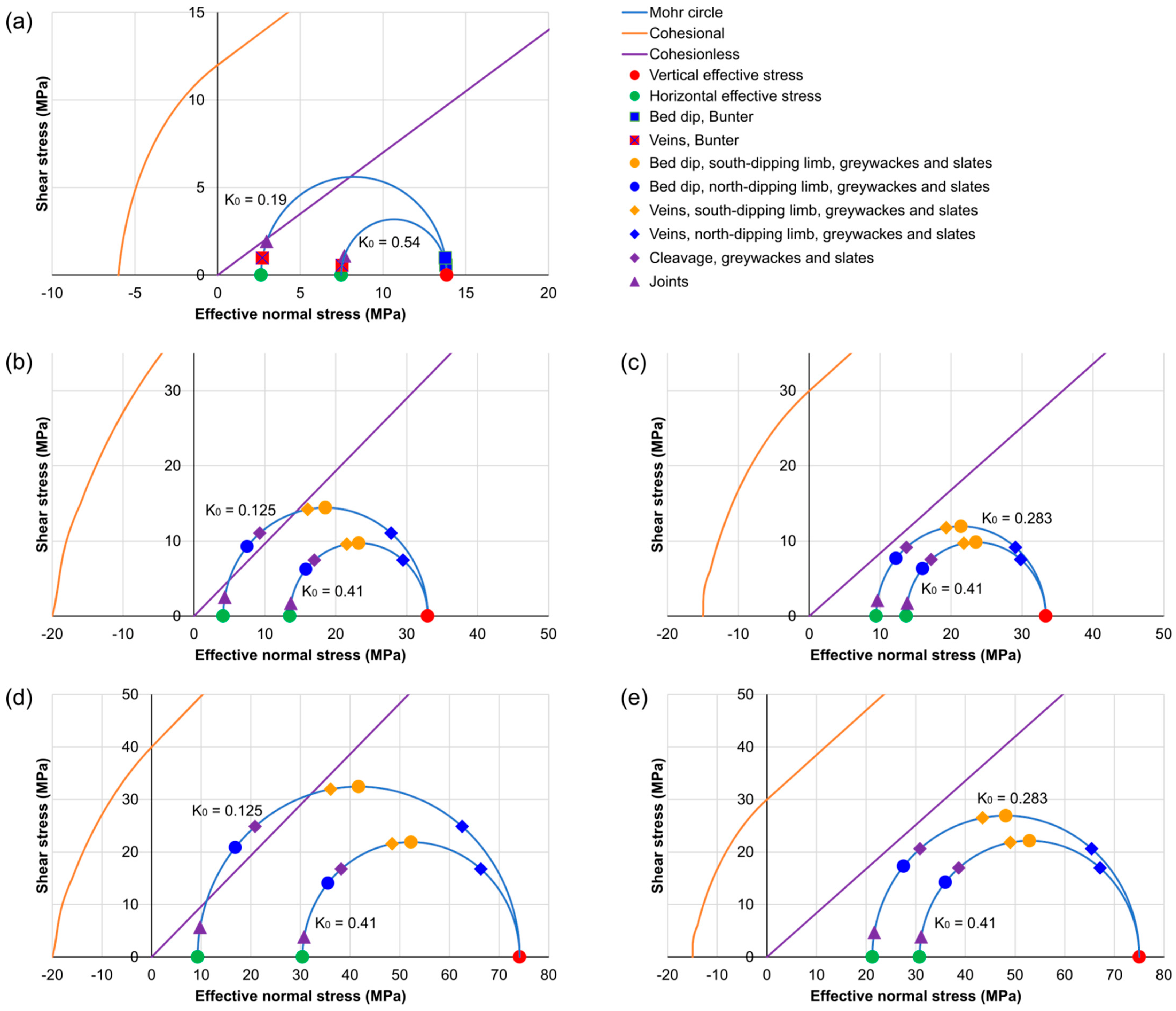
Very low geostatic stress ratios (e.g., 0.125) in the greywackes and slates are required to reactivate cohesionless fractures without fluid overpressure or applied tectonic stresses (base-case model; e.g., Figure 3a);
A fluid pressure of about 50 MPa would be needed to reactivate cohesionless fractures in both the greywackes and slates at a depth of 2 km if the geostatic stress ratio is high (e.g., 0.41; e.g., Figure 3b), with fluid pressures reaching lithostatic pressures;
Gently-dipping extension fractures will start to develop in the greywackes at a depth of 2 km if the fluid pressure is about 72 MPa, but may develop in the slates at slightly lower pressures (about 68 MPa). The models predict that, in the absence of cohesionless fractures, increasing fluid pressure will initially create gently-dipping extension fractures. This is because of the assumption of uniaxial strain (i.e., that the rocks are laterally confined). Higher fluid pressures will be required to generate steeply-dipping extension fractures, in the absence of horizontal tensile stresses, such as those related to tectonic forces or to cooling (Section 6);
Steeply-dipping extension fractures are predicted to develop in the greywackes at 2 km depth if there is a tensile tectonic stress between about −24 and −40 MPa, but are likely to develop in the slates at tensile tectonic stress between about −24 to −33 MPa (e.g., Figure 3d);
Extension fractures in all directions may develop in the greywackes at 2 km depth if the fluid pressure is between about 100 and 210 MPa, but would develop in the slates if the fluid pressure is between about 90 and 105 MPa (e.g., Figure 3e);
Shear (normal faulting) may begin on favourably-orientated cohesionless fractures in the greywackes at a depth of 2 km if there is a tensile tectonic stress between about 0 and −7.5 MPa, and in the slates if there is a tensile tectonic stress between about −2 and −6.5 MPa (e.g., Figure 3b);
Favourably-orientated cohesionless fractures may be reactivated as thrusts in the greywackes at 2 km depth if there is a compressive tectonic stress of about 170 MPa, and in the slates at about 140 MPa (e.g., Figure 3f);
New thrusts will begin to develop in the greywackes at a depth of 2 km if there is a compressive tectonic stress of about 360 MPa, but will develop in the slates if there is a compressive tectonic stress of about 270 MPa (e.g., Figure 3g).

The different critical values for the greywackes and slates predicted by the modelling are caused by the different physical properties that have been used for these rock types. The different geostatic stress ratios and failure criteria (especially cohesion and tensile strengths) are particularly important. The different geostatic stress ratios of different rock types may explain variations of fractures with lithology. This is commonly seen in greywacke/slate and sandstone/mudstone sequences (e.g., [96]). The tensile strengths of slates tend to be lower than that of greywackes, so extension fractures may develop in the slates at lower fluid pressures and lower tensile tectonic stresses than in the greywackes. Although this suggests that fractures will be created in slates before fracturing occurs in greywackes during stimulation (Section 6.1), it does not necessarily mean that there will be more, wider or better-connected fractures in the slates than in the greywackes. The model cannot predict the fluid flow properties of the slates or greywackes.

5.3. Possible Effects of Exhumation on the Bunter Sandstone

Here, we use simple modelling to determine at what depth joints are likely to have developed in the Bunter Sandstone of the Leinetal Graben, based on the changes in stresses and temperatures the rocks are likely to have experienced during exhumation. The Bunter Sandstone is currently exposed on the flanks of the Leinetal Graben but at depths of between ≈300 m and ≈850 m in Borehole Sudhein II in the Graben [37]. Note that the top of the Bunter Sandstone has been faulted out and the base is mixed with Zechstein Salt in Borehole Sudhein II [37]. The values used in the modelling are shown in Table 5, with the Mohr diagrams shown in Figure 6. The vertical stress changes as the thickness and, therefore, weight of the overlying material changes during burial or exhumation, and this causes a change in the horizontal stresses that is proportional to the geostatic stress ratio (Figure 4b). A change in depth typically causes a change in temperature that is related to the geothermal gradient (e.g., [97]). A decrease in temperature will tend to cause contraction of rock, determined by the coefficient of thermal expansion, and this will tend to cause a reduction in compressional stresses in the rock (e.g., [98]).

The model presented in Figure 6 includes reductions in horizontal stresses caused by decreases in overburden and temperature to predict at what depth extension fractures (e.g., joints) may develop in the Bunter Sandstone. We use a geothermal gradient of 30 °C per km, which is similar to that modelled by [99]. The model assumes, for simplicity, an initial 1.4 km depth for the top of the Bunter Sandstone, and an initial depth of 2 km for the base of the Bunter Sandstone (Figure 6a). Vertical and horizontal stresses reduce during exhumation, with the model predicting the development of joints beginning after 0.9 km exhumation, with the top of the Bunter at a depth of 0.5 km (Figure 6b). Note, however, that this base case model assumes hydrostatically-pressured pore fluids and no applied tectonic stresses. Joints would form at greater depths if the fluids are over-pressured, if there is a tensile tectonic stress, or if the geothermal gradient were higher.

Table 5. Initial values used for modelling the effects of exhumation and cooling on the Bunter Sandstone.

Parameter	Value	Unit
Density	2.68	g/cm³
Porosity	10	%
Tensile strength	6	MPa
Cohesion	12	MPa
Poisson ratio	0.25
Geostatic stress ratio	0.333
Young’s modulus	22	GPa
Coefficient of thermal expansion	11.25	10⁻⁶ °C⁻¹
Geothermal gradient	30	°C per km
Fluid pressure	Hydrostatic
Tectonic stresses	Zero
Initial top of unit	1.4	km
Initial base of unit	2	km

6. Discussion

6.1. Possible Effects of Stimulation on Devonian and Carboniferous Rocks at 2 km Depth

Here, we consider the possible effects of stimulation by increasing fluid pressure on the folded, cleaved and veined Devonian and Carboniferous greywackes and slates, based on the modelling discussed in Section 5 and using a simple schematic figure for these rocks (Figure 7a). The modelling suggests the following sequence of events as fluid pressure is gradually increased (Figure 7):

Favourably-orientated cohesionless fractures (joints) may be critically-stressed in greywackes with a very low geostatic stress ratio, so may undergo normal faulting even at hydrostatic fluid pressure (Figure 7a). Faulted joints are described by [100];
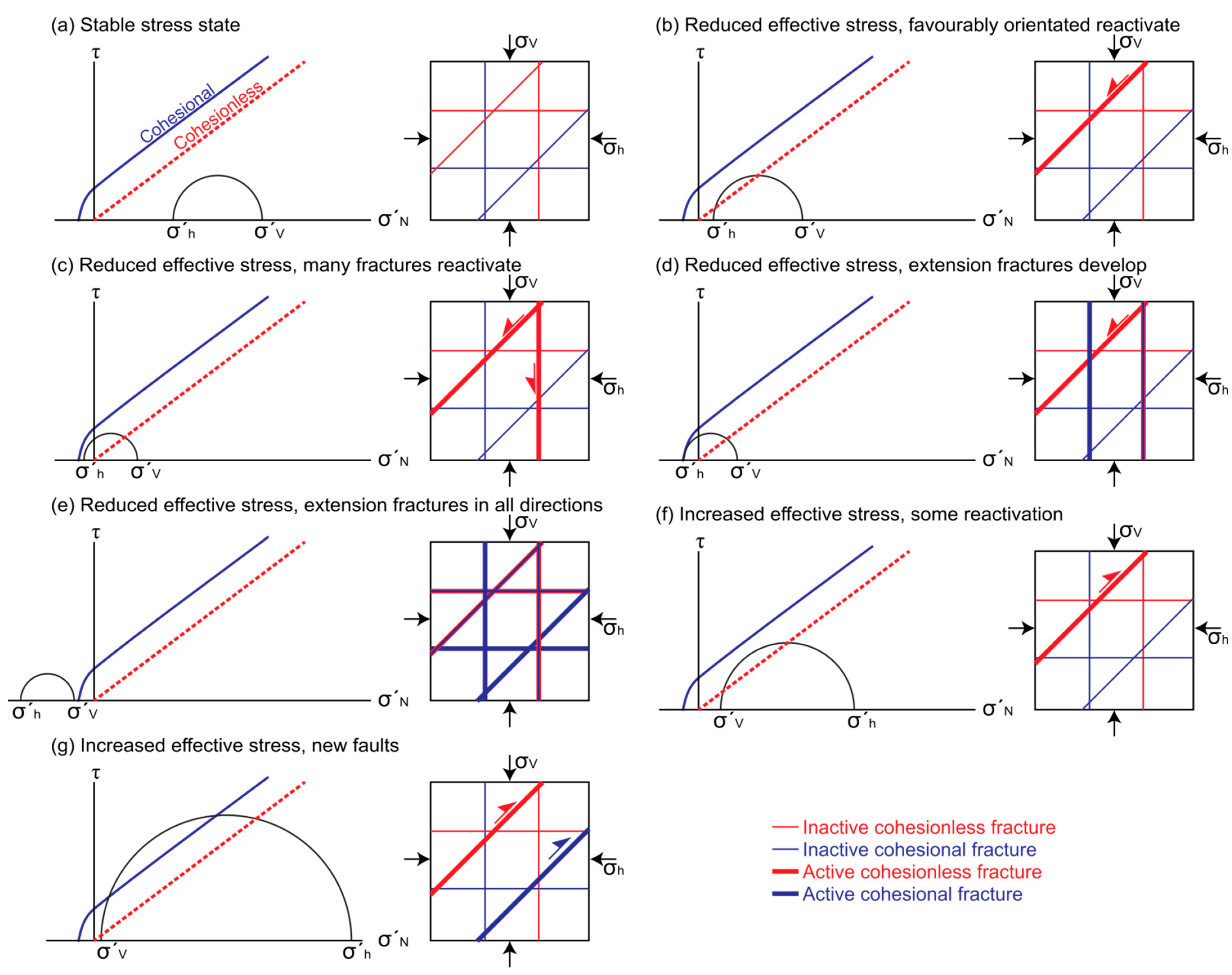
Shear can occur along favourably-orientated cohesionless fractures (e.g., joints) in the slates at fluid pressures of about 50 MPa, which is an overpressure of about 30 MPa (Figure 7b);
Gently-dipping extension fractures can be generated in the slates a fluid pressure of about 68 MPa, and gently-dipping cohesionless fractures in the greywackes may be reactivated as extension fractures (Figure 7c);
Gently-dipping extension fractures can be generated in the greywackes at a fluid pressure of about 72 MPa (Figure 7d);
Extension fractures with any orientation may develop in the slates at fluid pressure between about 90 and 105 MPa (Figure 7e);
Extension fractures with any orientation may develop in the greywackes if the fluid pressure is between about 100 and 210 MPa (Figure 6f).

6.2. Possible Effects of Stimulation on Devonian and Carboniferous Rocks at 4.5 km Depth

The critical values for deformation predicted by the modelling for the greywackes and slates at a depth of 4.5 km are shown in Table 4. These critical values are higher than predicted for a depth of 2 km, but suggest that stimulation would have similar effects as at a depth of 2 km. One notable difference is that higher differential stresses at depth would mean that stimulation is more likely to reactivate fractures in shear, or to create shear fractures, at greater depths. The modelling predicts that the slates will be particularly likely to develop shear fractures during stimulation.

Figure 8 highlights the effects of the different fluid pressures needed to stimulate reservoirs at different depths. The difference in fluid pressure between the top and bottom of a 2500 m column of water would be approximately 25 MPa. If fluid pressure is increased at a depth of 4.5 km such that it exceeds the horizontal stress, this may cause the fluid pressure at 2 km to exceed the vertical stress, if these different depths are hydraulically-connected (Figure 8). This suggests that care will be needed during stimulation if it is not intended to fracture rocks at shallower levels. We note that the Zechstein salts are likely to act as an effective top-seal (e.g., [101]) during stimulation.

6.3. Possibility of Open Fractures in the Devonian and Carboniferous Rocks below Göttingen

Although we have carried out simple modelling of joint development in the Bunter Sandstone, we have not performed so for the Devonian and Carboniferous rocks that are inferred to occur below about 1.5 km under Göttingen. This is because we consider there to be too many uncertainties for meaningful analysis of the effects of Late Cretaceous to Tertiary exhumation and cooling on these deeper and older rocks. There are, however, two arguments for the occurrence of open fractures in the Devonian and Carboniferous rocks. Firstly, joints will have developed in those rocks as they were exhumed at the end of the Variscan Orogeny, before deposition of the Permian and Mesozoic rocks unconformably above. It is possible, however, that these late- or post-Variscan joints will have subsequently been mineralised. Secondly, there is evidence that joints and other open fractures can occur at the depths of the proposed geothermal reservoir at Göttingen. For example, joints have been reported at depths of >2 km in tunnels (e.g., [102]) and in mines (e.g., [103,104]). Similarly, open fractures have been reported in fractured “basement” petroleum fields at depths of >4 km (e.g., [105]).

Figure 7. (previous page). Schematic figure for likely effects of stimulation on the folded and cleaved Devonian and Carboniferous greywackes and slates, based on the results presented in Table 4. The fold has an amplitude of a few metres to tens of metres. The model is for a depth of 2 km, at which hydrostatic fluid pressure would be 19.62 MPa. Veins are shown in the greywackes in the outer arcs of folds, and a fanning axial planar cleavage is shown. Joints are drawn approximately perpendicular to bedding. We predict the following sequence of events as fluid pressure is increased. (a) Favourably-orientated cohesionless fractures (joints) may be critically-stressed in greywackes with very low geostatic stress ratios, so may undergo normal faulting even at hydrostatic fluid pressure. (b) Shear can occur along favourably-orientated joints in the slates at fluid pressures of about 50 MPa. (c) Gently-dipping extension fractures can be generated in the slates at fluid pressures at about 68 MPa, and gently-dipping joints in the greywackes may be reactivated as extension fractures. (d) Extension fractures with any orientation may develop in the slates at fluid pressure between about 90 and 105 MPa. (e) Gently-dipping extension fractures can be generated in the greywackes at fluid pressures of about 72 MPa. (f) Extension fractures with any orientation may develop in the greywackes if the fluid pressure is between about 100 and 210 MPa.

Figure 8. Possible effects of stimulation at a depth of 4.5 km on the rocks at a depth of 2 km, modelled for a greywackes and slates with a geostatic stress ratio of 0.41. (a) Graph of pressure against depth. (b) Schematic cross-section. At a depth of 4.5 km, hydrostatic fluid pressure = 44.15 MPa, σ_V = 118.31 MPa and σ_h = 74.55 MPa. At a depth of 2 km, hydrostatic fluid pressure = 19.62 MPa, σ_V = 52.58 MPa and σ_h = 33.14 MPa. If there is hydraulic connectivity through the greywackes and slates, increasing fluid pressure at 4.5 km to above 77 MPa, such that it exceeds σ_h, would increase fluid pressure at 2 km 52.58 MPa, at which point it will equal σ_V.

6.4. Potential Benefits, Problems, and Improvements

Although the modelling presented in this paper is simple, it has several uses when attempting to predict what is likely to occur in the sub-surface. Firstly, constructing the models requires consideration of the range of the conditions that are likely to occur, including the lithologies and their mechanical properties, stresses, fluid types and fluid pressures, and the presence of different types of fractures. Secondly, predictions can be made about whether natural open fractures (e.g., joints) may occur, and whether exhumation might have created joints at reservoir depths. Thirdly, it enables predictions to be made about the orientations and types of induced fractures that are likely to occur under a range of possible conditions (Figure 7). It may also enable predictions to be made about whether there will be induced seismicity during stimulation.

There are various potential problems with the simplicity of the approach presented here, but these suggest ways in which the models can be improved. For example:

The Mohr diagram models used give little direct information about potential fluid flow in the sub-surface. The approach could, however, be used in combination with other modelling approaches. For example, it would be useful to compare predictions of critically stressed fractures from Mohr diagrams with distinct element analysis of fracture networks (e.g., [106,107]);
The values for rock properties used are based on triaxial tests, which are probably over-estimates because small, unfractured samples are generally used (e.g., [86]). More accurate methods for estimating the material properties of rock masses are available (e.g., [108]), and these methods could be used when more detailed information becomes available about the fracture patterns in the rock mass;
Similarly, we have used rock mechanical properties from the literature and have made various simplifying assumptions (e.g., no applied tectonic stresses, Biot coefficient = 1). The modelling can be improved and the assumptions properly tested as the input parameters become better constrained, for example as borehole data become available;
The anisotropy of the slates has not been modelled in a sophisticated way here, and this can be improved using more detailed information about the relationships between the angle between in situ stresses and cleavage (e.g., [109]);
The Mohr diagram analysis used here is two-dimensional, mainly because the magnitudes and orientations of the horizontal stresses are unknown. The analysis could be expanded to three dimensions when such information becomes available, for example from well data. Although predictions can be made about the stresses involved in the Variscan Orogeny and the formation of the Leinetal Graben, those predictions do not help with making predictions about the present-day stresses.

7. Conclusions

This paper shows how simple mechanical modelling, using Mohr diagrams and reasonable ranges of values for rock properties, stresses, and fluid pressures, can be used to predict fracturing in a potential geothermal reservoir. Inferences can be made about the range of structures likely to exist in the sub-surface and that may be generated during stimulation. Critical values of fluid pressure and applied tectonic stresses determine under what conditions different types and orientations of fractures are likely to occur or be generated during stimulation.

A model is presented for the development of shear and extension fractures in the Devonian and Carboniferous greywackes and slates as fluid pressure increases, as would occur during hydraulic stimulation (Figure 7). For a depth of 2 km, this involves: (a) shear on favourably-orientated cohesionless fractures in greywackes with a very low geostatic stress ratio under hydrostatic fluid pressure (Figure 7a); (b) shear along favourably-orientated joints in the slates at fluid pressures of about 50 MPa (Figure 7b); (c) generation of gently-dipping extension fractures in the slates at fluid pressures between about 68 MPa (Figure 7c); (d) development of gently-dipping extension fractures in the greywackes at fluid pressures of about 72 MPa (Figure 7d); (e) creation of extension fractures with any orientation in the slates at fluid pressure between about 90 and 105 MPa (Figure 7e); (f) Generation of fractures with any orientation in the greywackes at fluid pressures between about 100 and 210 MPa (Figure 7f). A similar sequence is predicted for a modelled depth of 4.5 km, although higher differential stresses at greater depths imply that hybrid or shear fractures are more likely to form than are extension fractures as fluid pressure increases.

The modelling addresses many key questions asked in Section 1. (1) The tensile strengths of slates tend to be lower than those of greywackes, suggesting lower fluid pressure or lower tensile tectonic stresses are needed to hydraulically fracture slates than greywackes. (2) Critical values of fluid pressure and tectonic stresses for fracturing can be predicted (Table 4). (3) Steeply-dipping cohesionless fractures (e.g., joints) are most likely to be reactivated first, as shear fractures. (4) Existing cohesionless fractures (e.g., joints) may initially reactivate in shear while cohesional fractures (e.g., veins) will tend to reactivate as extension fractures. (5) Shear fracturing generally requires the reactivation of cohesionless fractures as tensile tectonic stresses are applied, or the application of compressive tectonic stresses to generate new shear fractures. (6) Exhumation and related cooling may be responsible for the creation of joints in the Bunter Sandstone and the Variscan rocks beneath Göttingen. It is likely that joints developed in the Variscan rocks prior to deposition of the Permian rocks, but these may have subsequently been mineralised.

The relationships between stresses, fluid pressure and the types and orientations of fractures are important inputs for more detailed modelling techniques (e.g., DFN modelling [110]), and can be used to test the mechanical implications of those detailed modelling techniques. Not only does this modelling help geoscientists consider and model the ranges of mechanical properties of rock, stresses, fluid pressures and the resultant fractures that are likely to occur in the sub-surface, it encourages them to consider the ranges of key parameters and their effects.

Author Contributions

Conceptualization, D.C.P.P. and D.J.S.; methodology, D.C.P.P. and D.J.S.; software, D.J.S.; validation, D.C.P.P., D.J.S. and B.L.; resources, B.L.; data curation, B.L.; writing—original draft preparation, D.C.P.P.; writing—review and editing, D.J.S. and B.L.; supervision, B.L.; project administration, B.L.; funding acquisition, B.L. All authors have read and agreed to the published version of the manuscript.

Funding

This work has received funding from the European Union’s Horizon 2020 research and innovation programme (grant agreement № 792037-MEET Project).

Data Availability Statement

No new data were created or analysed in this study. Data sharing is not applicable to this article.

Acknowledgments

Carl-Heinz Friedel is thanked for helpful advice and discussions. We are grateful to John Reinecker and three anonymous reviewers, whose comments greatly improved this manuscript.

Conflicts of Interest

The authors declare no conflict of interest.

References

Leiss, B.; Tanner, D.; Vollbrecht, A.; Wemmer, K. Tiefengeothermisches Potential in der Region Göttingen—Geologische Rahmenbedingungen. In Neue Untersuchungen zur Geologie der Leinetalgrabenstruktur; Leiss, B., Tanner, D., Vollbrecht, A., Arp, G., Eds.; Universitätsverlag Göttingen: Göttingen, Germany, 2011; pp. 163–170. [Google Scholar]
Leiss, B.; Romanov, D.; Wagner, B. Risks and challenges of the transition to an integrated geothermal concept for the Göttingen University Campus. In Proceedings of the European Association of Geoscientists and Engineers, Conference Proceedings, 1st Geoscience and Engineering in Energy Transition Conference, Strasbourg, France, 16–18 November 2020; pp. 1–5. [Google Scholar] [CrossRef]
Leiss, B.; Wagner, B.; Heinrichs, T.; Romanov, D.; Tanner, D.C.; Vollbrecht, A.; Wemmer, K. Integrating deep, medium and shallow geothermal energy into district heating and cooling system as an energy transition approach for the Göttingen University Campus. In Proceedings of the World Geothermal Congress 2021, Reykjavik, Iceland, 24–27 October 2021; pp. 1–9. [Google Scholar]
Arp, G.; Vollbrecht, A.; Tanner, D.C.; Leiss, B. Zur Geologie des Leintalgrabens—Ein kurzer Überblick. In Neue Untersuchungen zur Geologie der Leinetalgrabenstruktur; Leiss, B., Tanner, D., Vollbrecht, A., Arp, G., Eds.; Universitätsverlag Göttingen: Göttingen, Germany, 2011; pp. 1–7. [Google Scholar]
Trullenque, G.; Genter, A.; Leiss, B.; Wagner, B.; Bouchet, R.; Léoutre, E.; Malnar, B.; Bär, K.; Rajšl, I. Upscaling of EGS in different geological conditions: a European perspective. In Proceedings of the 43rd Workshop on Geothermal Reservoir Engineering, Stanford University, Stanford, CA, USA, 12–14 February 2018. [Google Scholar]
Dalmais, E.; Genter, A.; Trullenque, G.; Leoutre, E.; Leiss, B.; Wagner, B.; Mintsa, A.C.; Bär, K.; Rajsl, I. MEET Project: toward the spreading of EGS across Europe. In Proceedings of the European Geothermal Congress, Den Haag, The Netherlands, 11–14 June 2019; p. 8. [Google Scholar]
Leiss, B.; Wagner, B.; MEET Konsortium. EU-Projekt MEET: Neue Ansätze »Enhanced Geothermal Systems (EGS)«—Göttinger Unicampus als Demoprojekt. Geotherm. Energ. 2020, 91, 26–28. [Google Scholar]
Welsch, B. Technical, Environmental and Economic Assessment of Medium Deep Borehole Thermal Energy Storage Systems. Ph.D. Thesis, Technische Universität Darmstadt, Darmstadt, Germany, 2019; 192p. [Google Scholar]
Krzywiec, P. Triassic-Jurassic evolution of the Pomeranian segment of the Mid-Polish Trough—Basement tectonics and subsidence patterns. Geol. Quart. 2006, 50, 139–150. [Google Scholar]
Doornenbal, H.; Stevenson, A. (Eds.) Petroleum Geological Atlas of the Southern Permian Basin Area; EAGE: Houten, The Netherlands, 2010; 342p. [Google Scholar]
Arp, G.; Hoffmann, V.E.; Seppelt, S.; Riegel, W. Trias und Jura von Göttingen und Umgebung. In Geobiologie 2—Jahrestagung der Paläontologischen Gesellschaft; Reitner, J., Reich, M., Schmidt, G., Eds.; Universitätsverlag Göttingen: Göttingen, Germany, 2004; Volume 74, pp. 147–192. [Google Scholar]
Leiss, B.; Tanner, D.; Vollbrecht, A.; Arp, G. (Eds.) Neue Untersuchungen zur Geologie der Leinetalgrabenstruktur; Universitätsverlag Göttingen: Göttingen, Germany, 2011; 170p. [Google Scholar]
Kirnbauer, T. (Ed.) Geologische Exkursionen in die Region um Göttingen; Jahresberichte und Mitteilungen des Oberrheinischen geologischen Vereins; E. Schweizerbart‘sche Verlagsbuchhandlung: Stuttgart, Germany, 2013; Volume 95, 319p. [Google Scholar]
Sanderson, D.J. Field-based structural studies as analogues to sub-surface reservoirs. In The Value of Outcrop Studies in Reducing Subsurface Uncertainty and Risk in Hydrocarbon Exploration and Production; Bowman, M., Smyth, H.R., Good, T.R., Passey, S.R., Hirst, J.P.P., Jordan, C.J., Eds.; Geological Society London, Special Publications: London, UK, 2015; Volume 436. [Google Scholar]
Martel, S.J. Progress in understanding sheeting joints over the past two centuries. J. Struct. Geol. 2017, 94, 68–86. [Google Scholar] [CrossRef] [Green Version]
Fairhurst, C. Fractures and fracturing: hydraulic fracturing in jointed rock. In Effective and Sustainable Hydraulic Fracturing; Jeffrey, R., Ed.; IntechOpen Limited: London, UK, 2013; pp. 47–79. ISBN 978-953-51-6341-1. [Google Scholar]
Ramsay, J.G. The Folding and Fracturing of Rocks; McGraw-Hill: New York, NY, USA, 1967; 568p. [Google Scholar]
Fossen, H. Structural Geology, 2nd ed.; Cambridge University Press: Cambridge, UK, 2016; 524p. [Google Scholar]
Mahmoodpour, S.; Singh, M.; Turan, A.; Bär, K.; Sass, I. Key parameters affecting the performance of fractured geothermal reservoirs: a sensitivity analysis by thermo-hydraulic-mechanical simulation. Geophysics. in review.
Friedel, C.H.; Huckriede, H.; Leiss, B.; Zweig, M. Large-scale Variscan shearing at the southeastern margin of the eastern Rhenohercynian belt: a reinterpretation of chaotic rock fabrics in the Harz Mountains, Germany. Int. J. Earth Sci. 2019, 108, 2295–2323. [Google Scholar] [CrossRef]
Fielitz, W. Variscan transpressive inversion in the northwestern central Rhenohercynian belt of western Germany. J. Struct. Geol. 1992, 14, 547–563. [Google Scholar] [CrossRef]
Franke, W. The mid-European segment of the Variscides: tectonostratigraphic units, terrane boundaries and plate tectonic evolution. In Orogenic Processes: Quantification and Modelling in the Variscan Belt; Franke, W., Haak, V., Oncken, O., Tanner, D., Eds.; Geological Society of London, Special Publications: London, UK, 2000; Volume 179, pp. 35–61. [Google Scholar]
Franke, W. Rheno-Hercynian belt of central Europe: review of recent findings and comparisons with south-west England. Geosci. SW Eng. 2007, 11, 263–272. [Google Scholar]
Friedel, C.H.; Hoffmann, C. Stopp 4: Schichtgebundene Deformationsstrukturen in der Kulmgrauwacke des Oberharzes (Bundesstraße 242). In Harzgeologie 2016. 5. Workshop Harzgeologie Kurzfassungen und Exkursionsführer; Friedel, C.H., Leiss, B., Eds.; Universitätsverlag Göttingen: Göttingen, Germany, 2016; pp. 85–90. [Google Scholar]
Zeuner, M. Conceptual 3D-Structure Model of the Variscan “Culm Fold Zone” in the Vicinity of the Oktertal dam (Harz Mountains, Germany) in Terms of Geothermal Reservoir Development. Master’s Thesis, Georg-August-Universität Göttingen, Göttingen, Germany, 2018. [Google Scholar]
Wagner, B.; Leiss, B.; Tanner, D.C. Stopp 2: Gefalteter unterkarbonischer Kieselschiefer am Bielstein nördlich Lautenthal (Innerstetal). In Harzgeologie 2016. 5. Workshop Harzgeologie Kurzfassungen und Exkursionsführer; Friedel, C.H., Leiss, B., Eds.; Universitätsverlag Göttingen: Göttingen, Germany, 2016; pp. 69–78. [Google Scholar]
Franzke, H.J.; Hauschke, N.; Hellmund, M. Spätpleistozäne bis holozäne Tektonik an der Harznordrand-Störung bei Benzingerode (Sachsen-Anhalt). In Harzgeologie 2016. 5. Workshop Harzgeologie Kurzfassungen und Exkursionsführer; Friedel, C.H., Leiss, B., Eds.; Universitätsverlag Göttingen: Göttingen, Germany, 2016; pp. 13–17. [Google Scholar]
De Graaf, S.; Lüders, V.; Banks, D.A.; Sośnicka, M.; Reijmer, J.J.G.; Kaden, H.; Vonhof, H.B. Fluid evolution and ore deposition in the Harz Mountains revisited: isotope and crush-leach analyses of fluid inclusions. Miner. Depos. 2020, 55, 47–62. [Google Scholar] [CrossRef] [Green Version]
Ramsey, J.M.; Chester, F.M. Hybrid fracture and the transition from extension fracture to shear fracture. Nature 2004, 428, 63–66. [Google Scholar] [CrossRef]
Wagner, B.; Günther, S.; Ford, K.; Sosa, G.; Leiss, B. The “Hexagon concept”: a fundamental approach for the geoscientific spatial data compilation and analysis at European scale to define the geothermal potential of Variscan and pre-Variscan low- to high-grade metamorphic and intrusive rocks. In Proceedings of the World Geothermal Congress 2021, Reykjavik, Iceland, 24–27 October 2021; pp. 1–10. [Google Scholar]
Arp, G.; Tanner, D.C.; Leiss, B. Struktur der Leinetalgraben-Randstörung bei Reiffenhausen (Autobahn 38 Heidkopftunnel-Westportal). In Neue Untersuchungen zur Geologie der Leinetalgrabenstruktur; Leiss, B., Tanner, D., Vollbrecht, A., Arp, G., Eds.; Universitätsverlag Göttingen: Göttingen, Germany, 2011; pp. 17–21. [Google Scholar]
Tanner, D.C. Exkursion nördliches Leinetal. In Neue Untersuchungen zur Geologie der Leinetalgrabenstruktur; Leiss, B., Tanner, D., Vollbrecht, A., Arp, G., Eds.; Universitätsverlag Göttingen: Göttingen, Germany, 2011; pp. 27–38. [Google Scholar]
Arp, G.; Bielert, F.; Hoffmann, V.E.; Löffler, T. Palaeoenvironmental significance of lacustrine stromatolites of the Arnstadt Formation (“Steinmergelkeuper”, Upper Triassic, N-Germany). Facies 2005, 51, 419–441. [Google Scholar] [CrossRef]
Ritter, M.; Vollbrecht, A.; van den Kerkhof, A.; Wemmer, K. Sedimentgänge im Bausandstein der Solling-Folge NW’ von Billingshausen. In Neue Untersuchungen zur Geologie der Leinetalgrabenstruktur; Leiss, B., Tanner, D., Vollbrecht, A., Arp, G., Eds.; Universitätsverlag Göttingen: Göttingen, Germany, 2011; pp. 89–106. [Google Scholar]
Reyer, D.; Bauer, J.F.; Philipp, S.L. Fracture systems in normal fault zones crosscutting sedimentary rocks, Northwest German Basin. J. Struct. Geol. 2012, 45, 38–51. [Google Scholar] [CrossRef]
Grupe, O. Uber die Zechsteinformation und ihr Salzlager im Untergrunde des hannoverschen Eichsfeldes und angrenzenden Leinegebietes nach den neueren Bohrergebnissen. Z. Fur Prakt. Geol. 1909, 17, 185–205. [Google Scholar]
Tanner, D.C.; Musmann, P.; Wawerzinek, B.; Buness, H.; Krawczyk, C.M.; Thomas, R. Salt tectonics of the eastern border of the Leinetal Graben, Lower Saxony, Germany, as deduced from seismic reflection data. Interpretation 2015, 3, T169–T181. [Google Scholar] [CrossRef]
Tanner, D.C.; Leiss, B.; Vollbrecht, A. Strukturgeologie des Leinetalgrabens (Exkursionen G1 und G2 am 4. und 5. April 2013); Jahresberichte und Mitteilungen des Oberrheinischen Geologischen Vereins Band; E. Schweizerbart’sche Verlagsbuchhandlung: Stuttgart, Germany, 2013; Volume 95, pp. 131–168. [Google Scholar]
Brink, H. The Variscan Deformation Front (VDF) in northwest Germany and its relation to a network of geological features including the ore-rich Harz Mountains and the European Alpine Belt. Int. J. Geosci. 2021, 12, 447–486. [Google Scholar] [CrossRef]
Vincent, C.J. Porosity of the Bunter Sandstone in the Southern North Sea Basin Based on Selected Borehole Neutron Logs; IR/05/074; British Geological Survey Internal Report: Keyworth, UK, 2005; 20p. [Google Scholar]
McNamara, D.D.; Faulkner, D.; McCarney, E. Rock properties of greywacke basement hosting geothermal reservoirs, New Zealand: preliminary results. In Proceedings of the Thirty-Ninth Workshop on Geothermal Reservoir Engineering Stanford University, Stanford, CA, USA, 24–26 February 2014. [Google Scholar]
Gholami, R.; Rasouli, V. Mechanical and elastic properties of transversely isotropic slate. Rock Mech. Rock Eng. 2013, 47. [Google Scholar] [CrossRef]
Menezes, F.F.; Lempp, C.; Svensson, K.; Neumann, A.; Pöllmann, H. Geomechanical behavior changes of Bunter Sandstone and borehole cement due to scCO₂ injection effects. In Proceedings of the IAEG/AEG Annual Meeting, San Francisco, CA, USA, 17–21 September 2018; Shakoor, A., Cato, K., Eds.; Springer Nature: Cham, Switzerland, 2019; Volume 1, pp. 111–118. [Google Scholar]
Agustawijaya, D.S. The uniaxial compressive strength of soft rock. Civil Eng. Dimen. 2007, 9, 9–14. [Google Scholar]
Menezes, F.F.; Lempp, C. On the structural anisotropy of physical and mechanical properties of a Bunter Sandstone. J. Struct. Geol. 2018, 114, 196–205. [Google Scholar] [CrossRef]
Havlíčková, D.; Závacký, M.; Krmíček, L. Anisotropy of mechanical properties of greywacke. GeoSci. Eng. 2019, 65, 46–52. [Google Scholar] [CrossRef]
Rodríguez-Sastre, M.A.; Gutiérrez-Claverol, M.; Torres-Alonso, M. Relationship between cleavage orientation, uniaxial compressive strength and Young’s modulus for slates in NW Spain. Bull. Eng. Geol. Environ. 2008, 67, 181–186. [Google Scholar] [CrossRef]
Price, N.J. Fault and Joint Development in Brittle and Semi-Brittle Rock; Pergamon Press: Oxford, UK, 1966; 176p. [Google Scholar]
Martel, S.J. Effects of cohesive zones on small faults and implications for secondary fracturing and fault trace geometry. J. Struct. Geol. 1997, 19, 835–847. [Google Scholar] [CrossRef]
Alneasan, M.; Behnia, M.; Bagherpour, H. The effect of Poisson’s ratio on the creation of tensile branches around dynamic faults. J. Struct. Geol. 2020, 131, 103950. [Google Scholar] [CrossRef]
Dobbs, M.R.; Cuss, R.J.; Ougier-Simonin, A.; Parkes, D.; Graham, C.C. Yield envelope assessment as a preliminary screening tool to determine carbon capture and storage viability in depleted southern north-sea hydrocarbon reservoirs. Int. J. Rock Mech. Min. Sci. 2018, 102, 15–27. [Google Scholar] [CrossRef]
Jefferies, G.M.; Crooks, J.H.A.; Becker, D.E.; Hill, P.R. Independence of geostatic stress from overconsolidation in some Beaufort Sea clays. Can. Geotech. J. 1987, 24, 342–356. [Google Scholar] [CrossRef]
Cai, J.; Du, G.; Ye, H.; Lei, T.; Xia, H.; Pan, H. A slate tunnel stability analysis considering the influence of anisotropic bedding properties. Adv. Mater. Sci. Eng. 2019, 2019, 4653401. [Google Scholar] [CrossRef] [Green Version]
Griffiths, L.; Heap, M.J.; Xu, T.; Chen, C.; Baud, P. The influence of pore geometry and orientation on the strength and stiffness of porous rock. J. Struct. Geol. 2017, 96, 149–160. [Google Scholar] [CrossRef]
Wang, H.; Mang, H.; Yuan, Y.; Pichler, B.L.A. Multiscale thermoelastic analysis of the thermal expansion coefficient and of microscopic thermal stresses of mature concrete. Materials 2019, 12, 2689. [Google Scholar] [CrossRef] [Green Version]
Pogacnik, J.; Elsworth, D.; O’Sullivan, M.; O’Sullivan, J. A damage mechanics approach to the simulation of hydraulic fracturing/shearing around a geothermal injection well. Comput. Geotech. 2016, 71, 338–351. [Google Scholar] [CrossRef]
Lee, C.; Park, J.W.; Park, C.; Park, E.S. Current status of research on thermal and mechanical properties of rock under high-temperature condition. Tunn. Undergr. Space 2015, 25, 1–23. [Google Scholar] [CrossRef] [Green Version]
Engelder, T.; Fischer, M.P. Influence of poroelastic behavior on the magnitude of minimum horizontal stress, S_h, in overpressured parts of sedimentary basins. Geology 1994, 22, 949–952. [Google Scholar] [CrossRef]
du Rouchet, J. Stress fields, a key to oil migration. AAPG Bull. 1981, 65, 74–85. [Google Scholar]
Mesri, G.; Hayat, T.M. The coefficient of earth pressure at rest. Can. Geotech. J. 1993, 30, 647–666. [Google Scholar] [CrossRef]
Gercek, H. Poisson’s ratio values for rocks. Int. J. Rock Mech. Min. Sci. 2007, 44, 1–13. [Google Scholar] [CrossRef]
Jaeger, J.C. Mohr diagram. In Structural Geology and Tectonics; Encyclopaedia of Earth Science; Springer: Berlin, Germany, 1987. [Google Scholar]
Hoek, E.; Martin, C.D. Fracture initiation and propagation in intact rock—A review. J. Rock Mech. Geotech. Eng. 2014, 6, 287–300. [Google Scholar] [CrossRef] [Green Version]
Anderson, E.M. The Dynamics of Faulting; Oliver & Boyd: Edinburgh, UK, 1951. [Google Scholar]
Cook, N.G.W. The failure of rock. Int. J. Rock Mech. Min. Sci. Geomech. Abs. 1965, 2, 389–403. [Google Scholar] [CrossRef]
Ucar, R. Determination of shear failure envelope in rock masses. J. Geot. Eng. 1986, 112, 303–315. [Google Scholar] [CrossRef]
Patel, S.; Martin, C.D. Effect of stress path on the failure envelope of intact crystalline rock at low confining stress. Minerals 2020, 10, 1119. [Google Scholar] [CrossRef]
Sibson, R.H. Brittle failure mode plots for compressional and extensional tectonic regimes. J. Struct. Geol. 1998, 20, 655–660. [Google Scholar] [CrossRef] [Green Version]
Brace, W.F. An extension of the Griffith theory of fracture to rocks. J. Geophys. Res. 1960, 65, 3477–3480. [Google Scholar] [CrossRef]
McClintock, F.A.; Walsh, J.B. Friction on Griffith cracks in rocks under pressure. In Proceedings of the fourth U.S. National Congress of Applied Mechanics, Berkeley, CA, USA, 18–21 June 1962; Volume 2, pp. 1015–1021. [Google Scholar]
Jaeger, J.C.; Cook, N.G.W. Fundamentals of Rock Mechanics; Methuen: London, UK, 1969; 515p. [Google Scholar]
Chang, C.; Zoback, M.D.; Khaksar, A. Empirical relations between rock strength and physical properties in sedimentary rocks. J. Pet. Sci. Eng. 2006, 51, 223–237. [Google Scholar] [CrossRef]
Zoback, M.D. Reservoir Geomechanics; Cambridge University Press: Cambridge, UK, 2007; 449p. [Google Scholar]
Sibson, R.H. A note on fault reactivation. J. Struct. Geol. 1985, 7, 751–754. [Google Scholar] [CrossRef]
Scholz, C.H. The Mechanics of Earthquakes and Faulting, 2nd ed.; Cambridge University Press: Cambridge, UK, 2002; 504p. [Google Scholar]
Meissner, R.; Strehlau, J. Limits of stresses in continental crusts and their relation to the depth-frequency distribution of shallow earthquakes. Tectonics 1982, 1, 73–89. [Google Scholar] [CrossRef]
Malama, B.; Kulatilake, P.H.S.W. Models for normal fracture deformation under compressive loading. Int. J. Rock Mech. Min. Sci. 2003, 40, 893–901. [Google Scholar] [CrossRef]
Corcoran, D.V.; Doré, A.G. Depressurization of hydrocarbon-bearing reservoirs in exhumed basin settings: evidence from Atlantic margin and borderland basins. In Exhumation of the North Atlantic Margin: Timing, Mechanisms and Implications for Hydrocarbon Exploration; Doré, A.G., Cartwright, J.A., Stoker, M.S., Turner, J.P., White, N., Eds.; Geological Society of London, Special Publications: London, UK, 2002; Volume 196, pp. 457–483. [Google Scholar]
Terzaghi, K. Erdbaumechanik auf Bodenphysikalischer Grundlage; Franz Deuticke: Vienna, Austria, 1925. [Google Scholar]
Terzaghi, K. Theoretical Soil Mechanics; Wiley: New York, NY, USA, 1943. [Google Scholar]
Bredehoeft, J.D.; Wesley, J.B.; Fouch, T.D. Simulations of the origin of fluid pressure, fracture generation, and the movement of fluids in the Uinta Basin, Utah. AAPG Bull. 1994, 78, 1729–1747. [Google Scholar]
Biot, M.A.; Willis, D.G. The elastic coefficients of the theory of consolidation. J. Appl. Mech. 1957, 24, 594–601. [Google Scholar] [CrossRef]
Barnhoorn, A.; Cox, S.F.; Robinson, D.J.; Senden, T. Stress- and fluid-driven failure during fracture array growth: implications for coupled deformation and fluid flow in the crust. Geology 2010, 38, 779–782. [Google Scholar] [CrossRef]
Crawford, B.R.; Webb, D.W.; Searles, K.H. Plastic compaction and anisotropic permeability development in unconsolidated sands with implications for horizontal well performance. In Proceedings of the 42nd US Rock Mechanics Symposium and 2nd U.S.-Canada Rock Mechanics Symposium, San Francisco, CA, USA, 29 June–2 July 2008. [Google Scholar]
Ferrill, D.A.; Smart, K.J.; Cawood, A.J.; Morris, A.P. The fold-thrust belt stress cycle: superposition of normal, strike-slip, and thrust faulting deformation regimes. J. Struct. Geol. 2021, 148, 104362. [Google Scholar] [CrossRef]
Becker, D.E. Testing in geotechnical design. Geotech. Eng. J. SEAGS AGSSEA 2010, 41, 10. [Google Scholar]
Bär, K.; Arbarim, R.; Turan, A.; Schulz, K.; Mahmoodpour, S.; Leiss, B.; Wagner, B.; Sosa, G.; Ford, K.; Trullenque, G.; et al. Database of Petrophysical and Fluid Properties and Recommendations for Model Parametrization of the Four Variscan Reservoir Types; MEET Report, Deliverable D5.5; MEET Consortium European, June 2020; 110p, Available online: https://www.meet-h2020.com/project-results/deliverables/ (accessed on 23 September 2021).
Tingay, M.R.P.; Hillis, R.R.; Morley, C.K.; Swarbrick, R.E.; Okpere, E.C. Variation in vertical stress in the Baram Basin, Brunei: tectonic and geomechanical implications. Mar. Pet. Geol. 2003, 20, 1201–1212. [Google Scholar] [CrossRef] [Green Version]
Tan, C.P.; Willoughby, D.R.; Zhou, S.; Hillis, R.R. An analytical method for determining horizontal stress bounds from wellbore data. Int. J. Rock Mech. Min. Sci. Geomech. Abs. 1993, 30, 1103–1109. [Google Scholar] [CrossRef]
Lund, B.; Townend, J. Calculating horizontal stress orientations with full or partial knowledge of the tectonic stress tensor. Geophys. J. Int. 2007, 170, 1328–1335. [Google Scholar] [CrossRef] [Green Version]
Zhang, J.; Hüpers, A.; Kreiter, S.; Kopf, A.J. Pore pressure regime and fluid flow processes in the shallow Nankai Trough Subduction Zone based on experimental and modeling results from IODP Site C0023. J. Geophys. Res. 2021, 126, e20248. [Google Scholar] [CrossRef]
Gao, B.; Flemings, P.B.; Nikolinakou, M.A.; Saffer, D.M.; Heidari, M. Mechanics of fold-and-thrust belts based on geomechanical modelling. J. Geophys. Res. 2018, 123, 4454–4474. [Google Scholar] [CrossRef]
Heidbach, O.; Rajabi, M.; Reiter, K.; Ziegler, M.; WSM Team. World Stress Map Database Release 2016. V. 1.1. GFZ Data Serv. 2016. [Google Scholar] [CrossRef]
Hobbs, B.E.; Means, W.D.; Williams, P.F. An Outline of Structural Geology; Wiley: New York, NY, USA, 1976; 671p. [Google Scholar]
Peacock, D.C.P.; Tavarnelli, E.; Anderson, M.W. Interplay between stress permutations and overpressure to cause strike-slip faulting during tectonic inversion. Terra Nova 2017, 29, 61–70. [Google Scholar] [CrossRef] [Green Version]
Laubach, S.E.; Olson, J.E.; Gross, M.R. Mechanical and fracture stratigraphy. AAPG Bull. 2009, 93, 1413–1426. [Google Scholar] [CrossRef]
Japsen, P.; Green, P.F.; Nielsen, L.H.; Rasmussen, E.S.; Bidstrup, T. Mesozoic-Cenozoic exhumation events in the eastern North Sea Basin: a multi-disciplinary study based on palaeothermal, palaeoburial, stratigraphic and seismic data. Basin Res. 2007, 19, 451–490. [Google Scholar] [CrossRef]
Nadan, B.J.; Engelder, T. Microcracks in New England granitoids: a record of thermoelastic relaxation during exhumation of intracontinental crust. Geol. Soc. Am. Bull. 2009, 121, 80–99. [Google Scholar] [CrossRef]
Albero, F.; Tanner, D.C. Modellierung des Temperaturfeldes um eine tiefe Förderbohrung am östlichen Rand des Leinetalgrabens—Abschätzung des geothermischen Potentials. In Neue Untersuchungen zur Geologie der Leinetalgrabenstruktur; Leiss, B., Tanner, D.C., Vollbrecht, A., Arp, G., Eds.; Universitätsverlag Göttingen: Göttingen, Germany, 2011; pp. 115–123. [Google Scholar]
Wilkins, S.J.; Gross, M.R.; Wacker, M.; Eyal, Y.; Engelder, T. Faulted joints: kinematics, displacement–length scaling relations and criteria for their identification. J. Struct. Geol. 2001, 23, 315–327. [Google Scholar] [CrossRef]
Karnin, W.D.; Idiz, E.; Merkel, D.; Ruprecht, E. The Zechstein Stassfurt Carbonate hydrocarbon system of the Thuringian Basin, Germany. Pet. Geosci. 1996, 2, 53–58. [Google Scholar] [CrossRef]
Bucher, K.; Stober, I.; Seelig, U. Water deep inside the mountains: unique water samples from the Gotthard rail base tunnel, Switzerland. Chem. Geol. 2012, 334, 240–253. [Google Scholar] [CrossRef]
Van Der Heever, P. The Influence of Geological Structure on Seismicity and Rockbursts in the Klerksdorp Goldfield. Master’s Thesis, Rand Afrikaans University, Johannesburg, South Africa, 1982; 156p. [Google Scholar]
Gumede, H.; Stacey, T.R. Measurement of typical joint characteristics in South African gold mines and the use of these characteristics in the prediction of rock falls. J. S. Afr. Inst. Min. Metall. 2007, 107, 335–344. [Google Scholar]
Areshev, E.G.; Dong, T.L.; San, N.T.; Shnip, O.A. Reservoirs in fractured basement on the continental shelf of southern Vietnam. J. Pet. Geol. 1992, 15, 451–464. [Google Scholar] [CrossRef]
Zhang, X.; Sanderson, D.J. Numerical study of critical behaviour of deformation and permeability of fractured rock masses. Mar. Pet. Geol. 1998, 15, 535–548. [Google Scholar] [CrossRef]
Camac, B.A.; Hunt, S.P. Predicting the regional distribution of fracture networks using the distinct element numerical method. AAPG Bull. 2009, 93, 1571–1583. [Google Scholar] [CrossRef]
Cundall, P.A.; Pierce, M.E.; Mas Ivars, D. Quantifying the size effect of rock mass strength. In Proceedings of the First Southern Hemisphere International Rock Mechanics Symposium, Perth, Australia, 16–19 September 2008; Potvin, Y., Carter, J., Dyskin., A., Jeffrey, R., Eds.; Australian Centre for Geomechanics: Perth, Australia, 2008; pp. 3–15. [Google Scholar]
Donath, F.A. Experimental study of shear failure in anisotropic rocks. Geol. Soc. Am. Bull. 1961, 72, 985–989. [Google Scholar] [CrossRef]
Yao, C.; Shao, J.F.; Jiang, Q.H.; Zhou, C. A new discrete method for modeling hydraulic fracturing in cohesive porous materials. J. Pet. Sci. Eng. 2019, 180, 257–267. [Google Scholar] [CrossRef]

Figure 4. Mohr diagrams showing the effects of key parameters on the failure envelope and state of effective stress, all shown using the model for the Devonian and Carboniferous greywackes with a geostatic stress ratio of 0.125. The parameters used are shown in Table 3. (a) The base case Mohr circle (depth of 2 km, hydrostatic fluid pressure and no applied tectonic stress), with a representative cohesional failure envelope shown (Table 3, “Greywacke” and “Slate” columns). “Friction angle” refers to the slope the failure envelope. (b) Mohr circles for effective stress at different depths (hydrostatic fluid pressure and no applied tectonic stress). The magnitudes of the effective stresses increase with depth. (c) Mohr circles for a depth of 2 km, hydrostatic fluid pressure and different applied tectonic stresses. (d) Mohr circles for a depth of 2 km, different fluid pressures and zero applied tectonic stresses.

Figure 6. Mohr diagrams illustrating the possible effects of exhumation and cooling on the Bunter Sandstone. See Table 5 for parameters used in the model. (a) Model for the base of the Bunter Sandstone at a depth of 2 km and the top of the Bunter Sandstone at 1.4 km. The model predicts the rock is in a stable stress state. (b) Model for the Bunter Sandstone after 0.9 km exhumation. The top of the Bunter Sandstone is now at a depth of 0.5 km, and the stress state promotes the development of steeply-dipping extension fractures. Notice that the differential effecting stresses in (a,b) are similar, because cooling during exhumation tends to generate horizontal tensile stresses.

Table 2. Parameters used in the modelling. * Geostatic stress ratios are calculated from the Poisson ratios. ** Representative values of the coefficient of internal friction are used here, using the approximate median value of the range of internal angles of friction.

	Definition and significance	Bunter sandstone	Greywacke	Slate	Unit
Density	The mass per unit volume of the rock and/or the fluids in the rock. Mean density controls the vertical (overburden) stress	2.68 [40]	2.42 to 2.74 [41]	2.7 to 2.9 [42]	g/cm³
Tensile strength	The stress needed to cause extension fracturing. Controls where the failure envelope intersects the zero shear stress axis of the Mohr diagram, and the magnitudes of the effective tensile stresses needed to create extension fractures	6 [43]	20.3 to 35.7 [41]	4.4 normal to cleavage,14.4 along cleavage [42]	MPa
Uniaxial compressive strength	The strength of a rock derived from a uniaxial compression test (e.g., [44])	70 to 134 [45]	Average ≈ 200 (range 41–209) [46]	2.33 to 151.6 [47]	MPa
Cohesion	The shear strength of a material when the stress normal to a shear surface is zero (e.g., [48,49]). Controls where the failure envelope intersects the zero normal stress axis of the Mohr diagram, and the magnitudes of the effective differential stresses needed to create shear fractures	12 [45]	49 to 51 [41]	64 normal to cleavage, 11 when σ₁ 30° to cleavage [42]	MPa
Poisson ratio	The relationship between the tendency to shorten in one direction and the tendency to expand in another direction (e.g., [50])	0.16 to 0.35 [51]	0.11 to 0.29 [41]	0.22 to 0.29 [42]
Geostatic stress ratio *	The ratio of the horizontal effective stress (σ′_H) to the vertical effective stress (σ′_V) (e.g., [52]). It gives the effect the overburden has on horizontal stresses. Influences the diameter of the Mohr circle. Values calculated using Equation (2)	0.19 to 0.54	0.125 to 0.41 [41]	0.28 to 0.41
Angle of internal friction (φ)	The angle of the fracture to σ₁ is ± (45° − φ/2) (e.g., [48])	27.6 to 37.9 [51]	43 to 44 [41]	30 to 50 [53]	Degrees
Coefficient of internal friction (μ) **	Controls the slope of the failure envelope in the compressional field of the Mohr diagram (e.g., [48]). μ = tan φ	0.52	0.97	0.84
Young’s modulus	The stiffness of a solid material (e.g., [54])	22 to 37 [51]	2.3 to 7 [41]	12 to 56 [42]	GPa
Coefficient of thermal expansion	The extent to which a material expands when heated or contracts when cooled. Can influence the development of tensile stresses during exhumation and cooling of rocks	11.25 [55]	17 [56]	8 [57]	10⁻⁶ K⁻¹

Table 3. Parameters used to model the base case scenarios for the Bunter Sandstone and the Devonian and Carboniferous greywackes and slates, with stresses and fluid pressures rounded to one decimal place. Values that depend on different geostatic stress ratios (k₀) are shown in different colours (red for lower k₀ values in range, blue for upper k₀ values). Values specific to a modelled depth of 2 km are shown in bold, and values specific to a modelled depth of 4.5 km are shown in italics. Representative structures are shown for the dips of structures in both the SE- and NW-dipping limbs of folds in the greywackes and slates. Effective stresses are calculated assuming a Biot coefficient of 1.

		Bunter	Greywacke	Slate	Unit
Input parameters	Depth	1000	2000 4500	2000 4500	m
	Average rock density	2.41	2.68	2.68	g/cm³
	Fluid density	1	1	1	g/cm³
	Overpressure	0	0	0	MPa
	Poisson’s ratio (ν)	0.16	0.11, 0.29	0.22, 0.29	0.16
	Applied tectonic stress	0	0	0	MPa
	Cohesion	12	40	30	MPa
	Coefficient of internal friction (μ)	0.7	0.97	0.84
	Friction angle	33	44	40	Degrees
	Tensile strength (T)	6	20	15	MPa
	Bed dip	5	SE limb = 45° NW limb = 70°	SE limb = 45° NW limb = 70°	Degrees
	Vein dip	85	SE limb = 45° NW limb = 25°	S limb = 45° NW limb = 25°	Degrees
	Cleavage	N/A	65	65	Degrees
	Joint dip	90	85	85	Degrees
Derived parameters	Fluid pressure	9.81	19.6 44.1	19.6 44.1	MPa
	Geostatic pressure ratio (k₀)	0.19	0.125, 0.41	0.283, 0.41
	Vertical effective stress ( σ′_V)	13.85	33 74.2	33.4 75.1	MPa
	Horizontal effective stress (σ′_H =σ´_V k₀)	2.63	4.1, 13.5 9.3, 30.4	9.4, 13.7 21.2, 30.8	MPa

Publisher’s Note: MDPI stays neutral with regard to jurisdictional claims in published maps and institutional affiliations.

© 2021 by the authors. Licensee MDPI, Basel, Switzerland. This article is an open access article distributed under the terms and conditions of the Creative Commons Attribution (CC BY) license (https://creativecommons.org/licenses/by/4.0/).

Share and Cite

MDPI and ACS Style

Peacock, D.C.P.; Sanderson, D.J.; Leiss, B. Use of Mohr Diagrams to Predict Fracturing in a Potential Geothermal Reservoir. Geosciences 2021, 11, 501. https://doi.org/10.3390/geosciences11120501

AMA Style

Peacock DCP, Sanderson DJ, Leiss B. Use of Mohr Diagrams to Predict Fracturing in a Potential Geothermal Reservoir. Geosciences. 2021; 11(12):501. https://doi.org/10.3390/geosciences11120501

Chicago/Turabian Style

Peacock, D.C.P., David J. Sanderson, and Bernd Leiss. 2021. "Use of Mohr Diagrams to Predict Fracturing in a Potential Geothermal Reservoir" Geosciences 11, no. 12: 501. https://doi.org/10.3390/geosciences11120501

Note that from the first issue of 2016, this journal uses article numbers instead of page numbers. See further details here.

Article Menu

Use of Mohr Diagrams to Predict Fracturing in a Potential Geothermal Reservoir

Abstract

1. Introduction

2. Predictions about the Pre-Permian Geology beneath Göttingen

3. Model Set-Up

3.1. Mohr Diagrams, Stresses and Failure Envelopes

3.2. Input Data, Assumptions, and Uncertainties

3.3. Base Case Models

3.4. A Range of Stress States for Fracturing

4. Effects of Key Parameters

5. Potential for Reactivating and Generating Fractures

5.1. Bunter Sandstone

5.2. Devonian and Carboniferous Greywackes and Slates

5.3. Possible Effects of Exhumation on the Bunter Sandstone

6. Discussion

6.1. Possible Effects of Stimulation on Devonian and Carboniferous Rocks at 2 km Depth

6.2. Possible Effects of Stimulation on Devonian and Carboniferous Rocks at 4.5 km Depth

6.3. Possibility of Open Fractures in the Devonian and Carboniferous Rocks below Göttingen

6.4. Potential Benefits, Problems, and Improvements

7. Conclusions

Author Contributions

Funding

Data Availability Statement

Acknowledgments

Conflicts of Interest

References

Share and Cite

Article Metrics

Article Access Statistics

Further Information

Guidelines

MDPI Initiatives

Follow MDPI