Demand Response in HEMSs Using DRL and the Impact of Its Various Configurations and Environmental Changes

Abstract

With smart grid advances, enormous amounts of data are made available, enabling the training of machine learning algorithms such as deep reinforcement learning (DRL). Recent research has utilized DRL to obtain optimal solutions for complex real-time optimization problems, including demand response (DR), where traditional methods fail to meet time and complex requirements. Although DRL has shown good performance for particular use cases, most studies do not report the impacts of various DRL settings. This paper studies the DRL performance when addressing DR in home energy management systems (HEMSs). The trade-offs of various DRL configurations and how they influence the performance of the HEMS are investigated. The main elements that affect the DRL model training are identified, including state-action pairs, reward function, and hyperparameters. Various representations of these elements are analyzed to characterize their impact. In addition, different environmental changes and scenarios are considered to analyze the model’s scalability and adaptability. The findings elucidate the adequacy of DRL to address HEMS challenges since, when appropriately configured, it successfully schedules from 73% to 98% of the appliances in different simulation scenarios and minimizes the electricity cost by 19% to 47%.

1. Introduction

To address complex challenges in power systems associated with the presence of distributed energy resources (DERs), wide application of power electronic devices, increasing number of price-responsive demand participants, and increasing connection of flexible load, e.g., electric vehicles (EV) and energy storage systems (ESS), recent studies have adopted artificial intelligence (AI) and machine learning (ML) methods as problem solvers [1]. AI can help overcome the aforementioned challenges by directly learning from data. With the spread of advanced smart meters and sensors, power system operators are producing massive amounts of data that can be employed to optimize the operation and planning of the power system. There has been increasing interest in autonomous AI-based solutions. The AI methods require little human interaction while improving themselves and becoming more resilient to risks that have not been seen before.

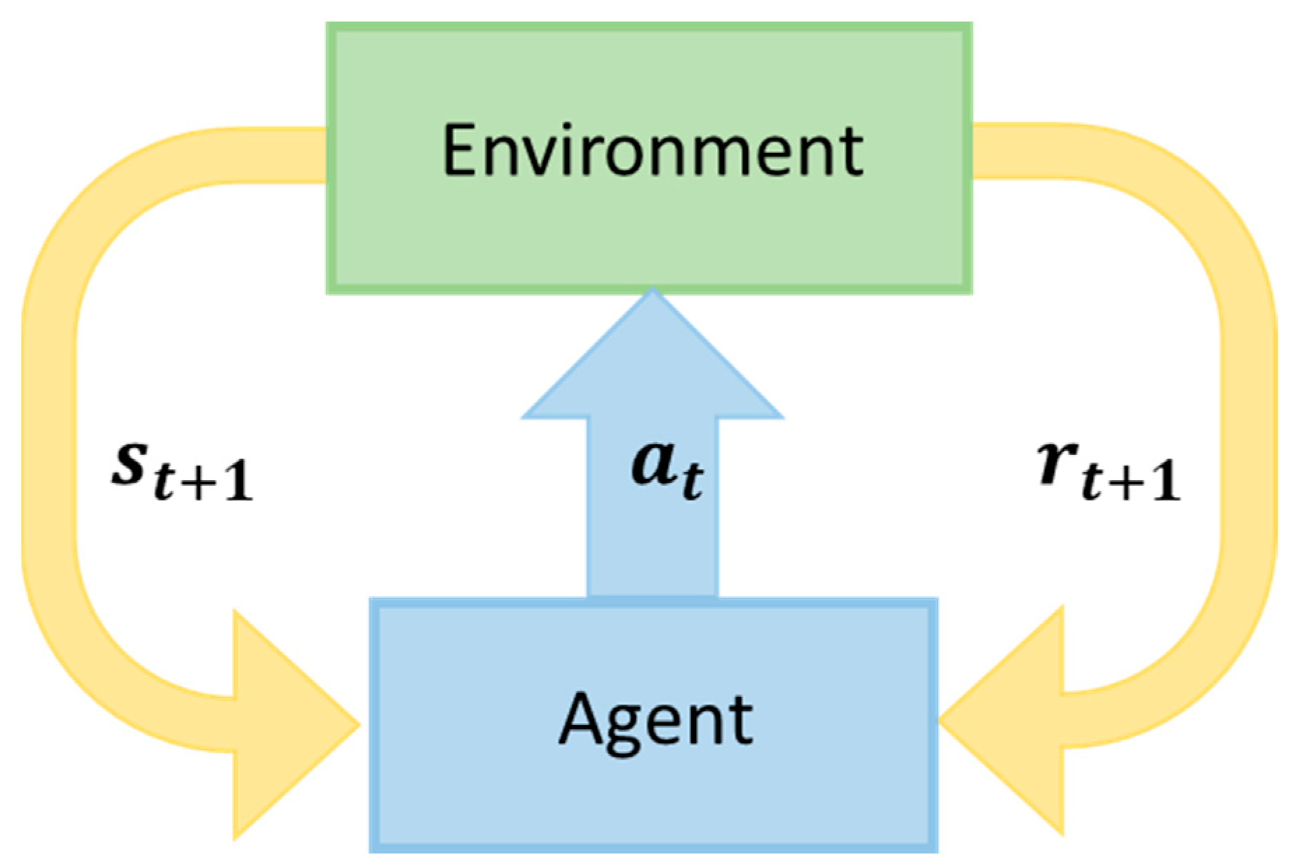
Recently, reinforcement learning (RL) and deep reinforcement learning (DRL) have become popular approaches to optimize and control the power system operation, including demand-side management [2], the electricity market [3], and operational control [4], among others. RL learns the optimal actions from data through continuous interactions with the environment, while the global optimum is unknown. It eliminates the dependency on accurate physical models by learning a surrogate model. It identifies what works better with a particular environment by assigning a numeric reward or penalty to the action taken after receiving feedback from the environment. In contrast to the performance of RL, the conventional and model-based DR approaches, such as mixed interlinear programming [5,6], mixed integer non-linear programming (MINLP) [7], particle swarm optimization (PSO) [8], and Stackelberg PSO [9], require accurate mathematical models and parameters, the construction of which is challenging because of the increasing system complexities and uncertainties.

In demand response (DR), RL has shown effectiveness by optimizing the energy consumption for households via home energy management systems (HEMSs) [10]. The motivation behind applying DRL for DR arises mainly from the need to optimize a large number of variables in real time. The deployment of smart appliances in households is rapidly growing, increasing the number of variables that need to be optimized by the HEMS. In addition, the demand is highly fluctuant due to the penetration of EVs and RESs in the residential sector [11]. Thus, new load scheduling plans must be processed in real-time to satisfy the users’ needs and adapt to their lifestyles by utilizing their past experiences. RL has been proposed for HEMSs, demonstrating the potential to outperform other existing models. Initial studies focused on proof of concept, with research such as [12,13] advocating for its ability to achieve better performance than traditional optimization methods such as MILP [14], genetic algorithms [15], and PSO [16].

More recent studies focused on utilizing different learning algorithms for HEMS problems, including deep Q-networks (DQN) [17], double DQN [18], deep deterministic policy gradients [19], and a mixed DRL [20]. In [21], the authors proposed a multi-agent RL methodology to guarantee optimal and decentralized decision-making. To optimize their energy consumption, each agent corresponded to a household appliance type, such as fixed, time-shiftable, and controllable appliances. Additionally, RL was utilized to control heating, ventilation, and air conditioning (HVAC) loads in the absence of thermal modeling to reduce electricity cost [22,23]. Work in [24] introduces an RL-based HEMS model that optimizes energy usage considering DERs such as ESS and a rooftop PV system. Lastly, many studies have focused on obtaining an energy consumption plan for EVs [25,26]. However, most of these studies only look at improving their performance compared to other approaches without providing precise details, such as the different configurations of the HEMS agent based on an RL concept or hyperparameter tuning for a more efficient training process. Such design, execution, and implementation details can significantly influence HEMS performance. DRL algorithms are quite sensitive to their design choices, such as action and state spaces, and their hyperparameters, such as neural network size, learning and exploration rates, and others [27].

The DRL adoption in real-world tasks is limited because of the reward design and safe learning. There is a lack in the literature of in-depth technical and quantitative descriptions and implementation details of DRL in HEMSs. Despite the expert knowledge required in DR and HEMS, DRL-based HEMSs pose extra challenges. Hence, a performance analysis of these systems needs to be conducted to avoid bias and gain insight into the challenges and the trade-offs. The compromise between the best performance metrics and the limiting characteristics of interfacing with different types of household appliances, EV, and ESS models will facilitate the successful implementation of DRL in DR and HEMS. Further, there is a gap in the literature regarding the choice of reward function configuration in HEMSs, which is crucial for their successful deployment.

In this paper, we compare different reward functions for DRL-HEMS and test them using real-world data. In addition, we examine various configuration settings of DRL and their contributions to the interpretability of these algorithms in HEMS for robust performance. Further, we discuss the fundamental elements of DRL and the methods used to fine-tune the DRL-HEMS agents. We focus on DRL sensitivity to specific parameters to better understand their empirical performance in HEMS. The main contributions of this work are summarized as follows:

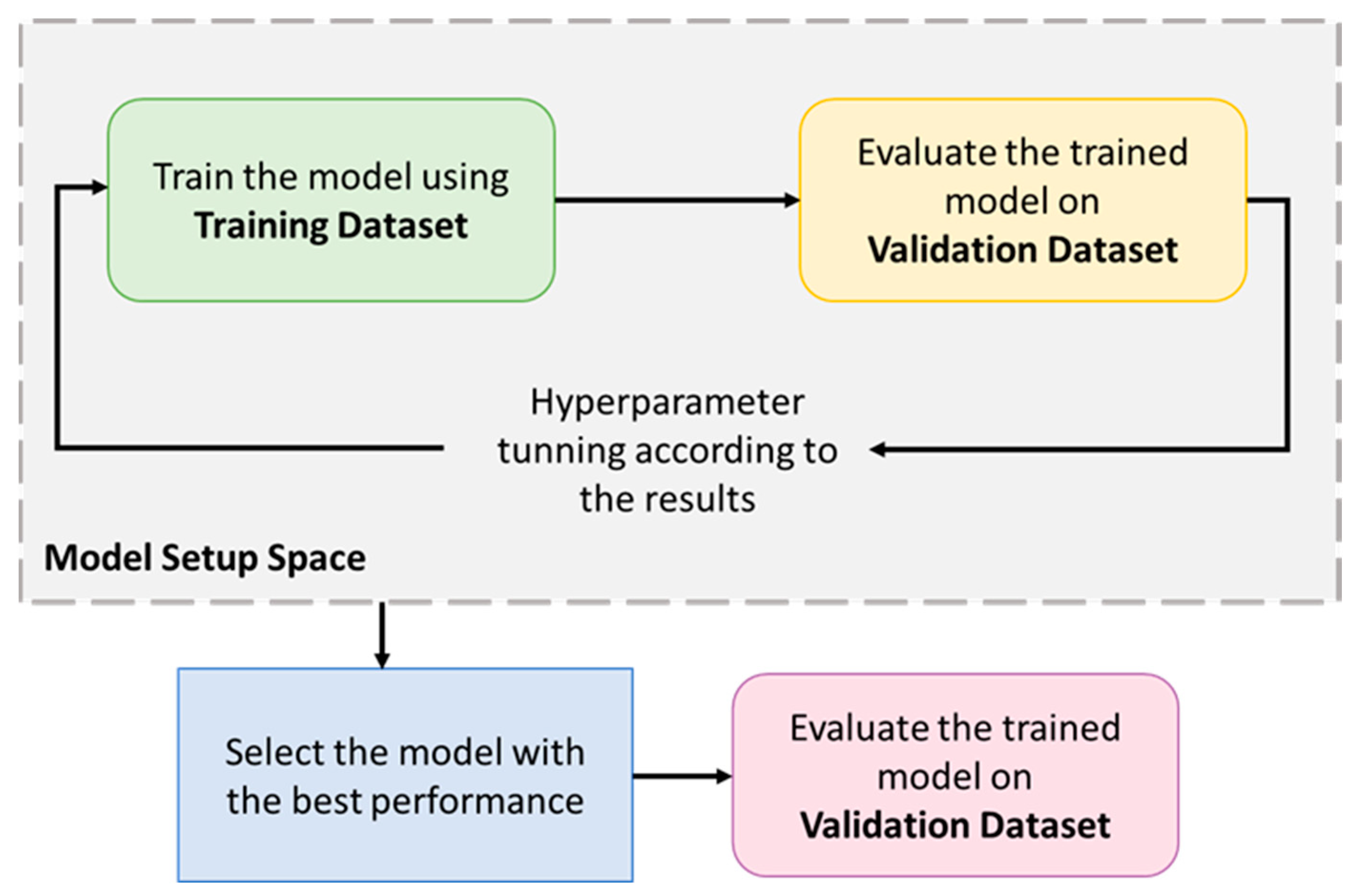
• A study of the relationship between training and deployment of DRL is presented. The implementation of the DRL algorithm is described in detail with different configurations regarding four aspects: environment, reward function, action space, and hyperparameters.
• We have considered a comprehensive view of how the agent performance depends on the scenario considered to facilitate real-world implementation. Various environments account for several scenarios in which the state-action pair dimensions are varied or the environment is made non-stationary by changing the user’s behavior.
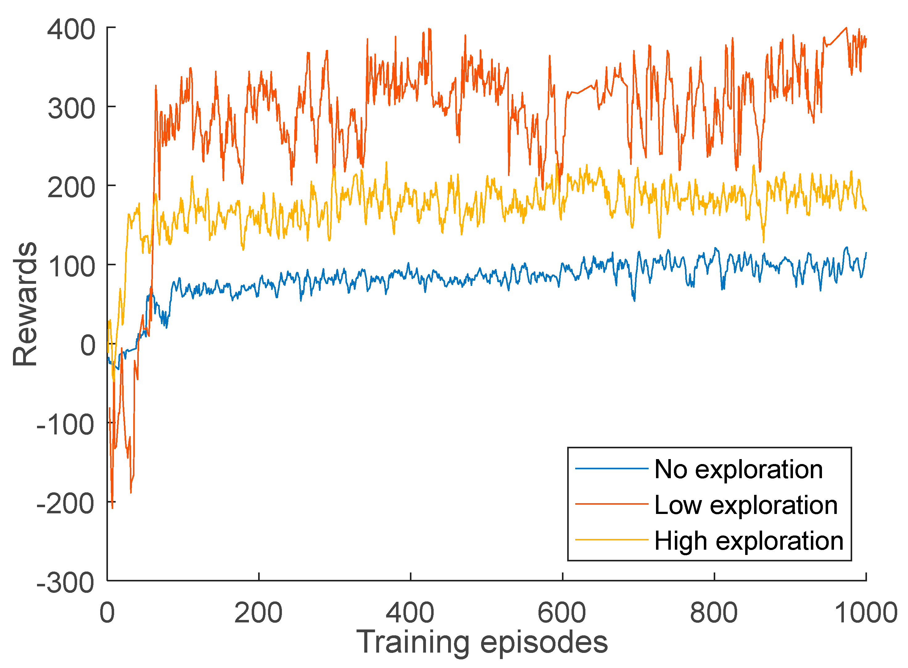
• Extensive simulations are conducted to analyze the performance when the model hyperparameters are changed (e.g., learning rates and discount factor). This verifies the validity of having the model representation as an additional hyperparameter in applying DRL. To this end, we choose the DR problem in the context of HEMS as a use case and propose a DQN model to address it.

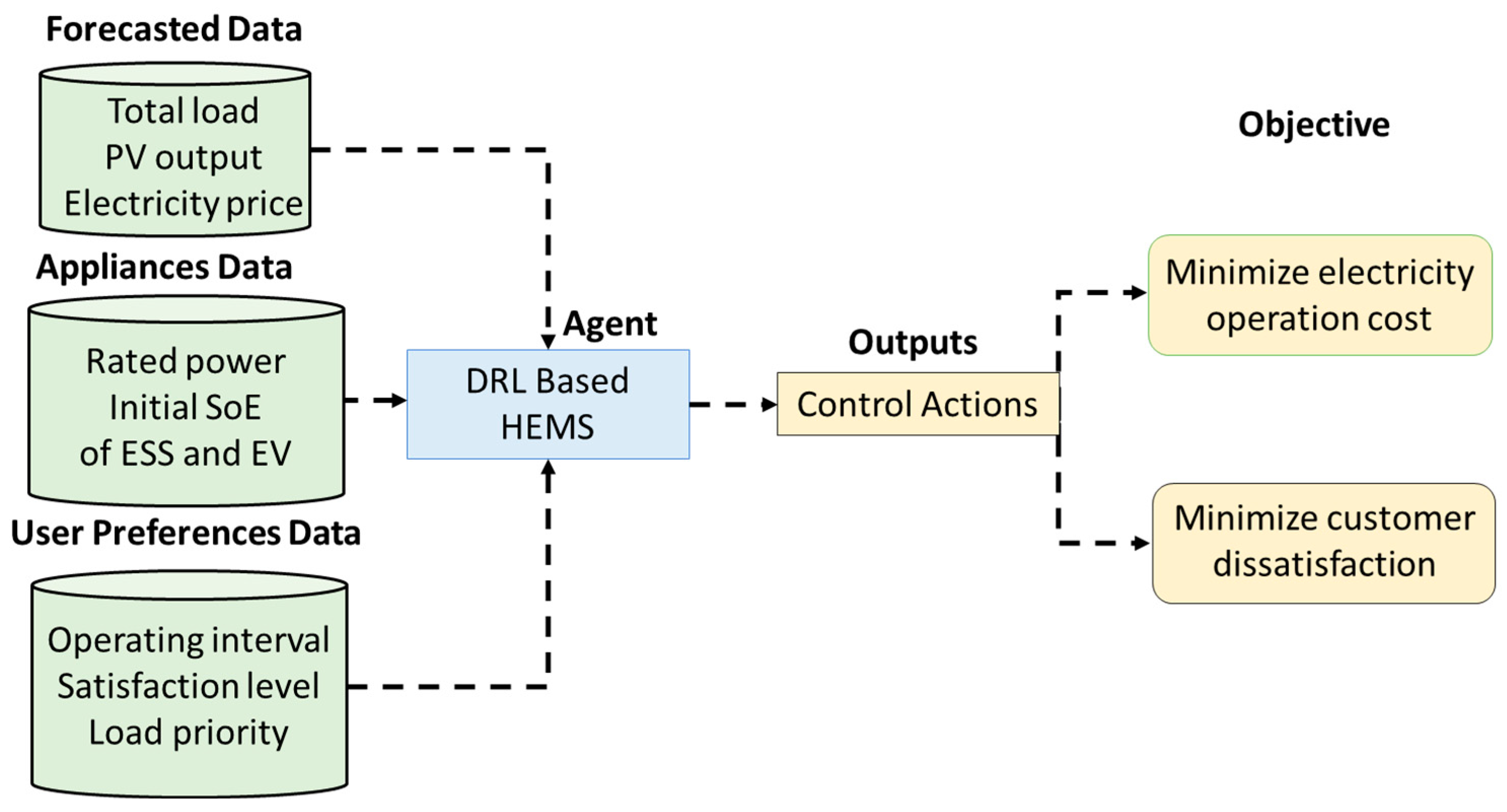
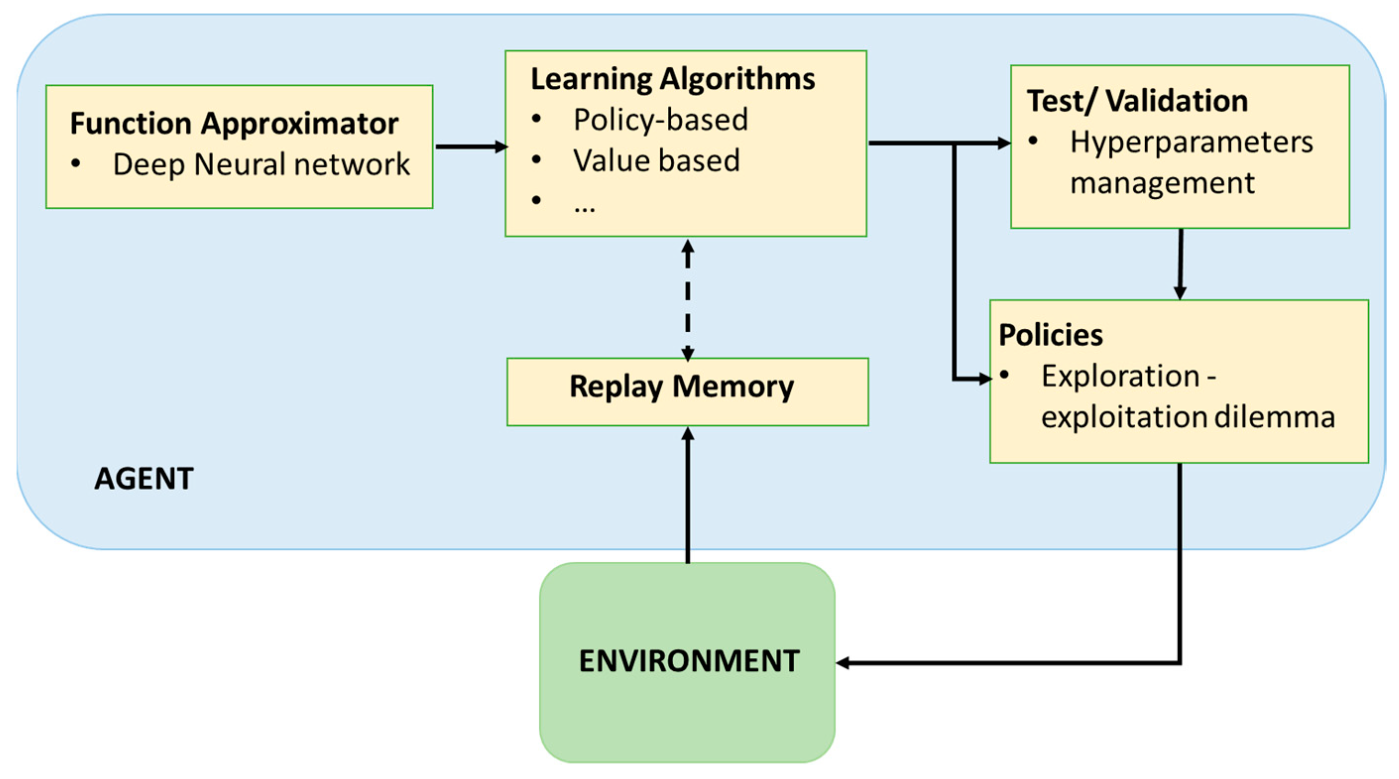
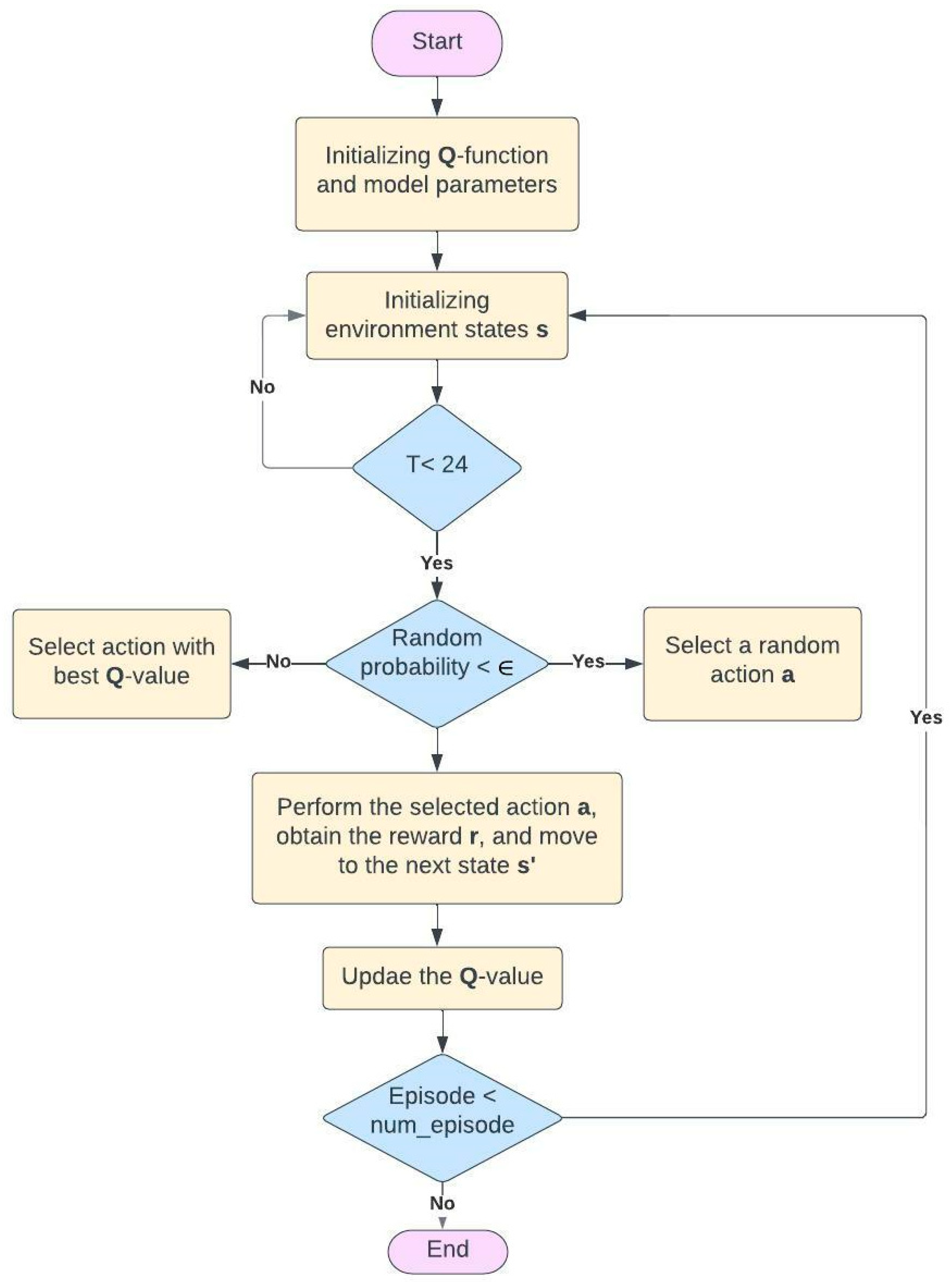
The remainder of this paper is structured as follows. The DR problem formulation with various household appliances is presented in Section 2. Section 3 presents the DRL framework, different configurations to solve the DR problem, and the DRL implementation process. Evaluation and analysis of the DRL performance results are discussed in Section 4. Concluding along with the future work and limitation remarks are presented in Section 5.

2. Demand Response Problem Formulation

The advances in smart grid technologies enable power usage optimization for customers by scheduling their different loads to minimize the electricity cost considering various appliances and assets, as shown in Figure 1. The DR problem has been tackled in different studies; however, the flexible nature of the new smart appliances and the high-dimensionality issue add a layer of complexity to it. Thus, new algorithms and techniques, such as DRL, are proposed to address the problem. The total electricity cost is minimized by managing the operation of different categories of home appliances. The appliances’ technical constraints and user comfort limit the scheduling choices. Thus, the DR problem is defined according to the home appliances’ configuration and their effect on user comfort. The home appliances can be divided into three groups as follows:

2.1. Shiftable Appliances

The working schedule of this appliance group can be changed, e.g., from a high-price time slot to another lower-price time slot, to minimize the total electricity cost. Examples of this type are washing machines (WMs) and dishwashers (DWs). The customer’s discomfort may be endured due to waiting for the appliance to begin working. Assume a time-shiftable appliance requires an interval of $d_n$ to achieve one operation cycle. The time constraints of the $n$ shiftable appliance are defined as:

$$t_{int,n}\le t_{start,n} \le \left(t_{end,n}-d_n\right)$$

(1)

2.2. Controllable, Also Known as Thermostatically Controlled, Appliances

This group of appliances includes air conditioners (ACs) and water heaters (WHs), among others, in which the temperature can be adjusted by the amount of electrical energy consumed. Their consumption can be adjusted between maximum and minimum values in response to the electricity price signal, as presented in (2). Regulating the consumption of these appliances reduces charges on the electricity bill. However, reduced consumption can affect the customer’s thermal comfort. The discomfort is defined based on the variation $\left(E_n^{max}-E_{n,t}\right)$. When this deviation decreases, customer discomfort decreases and vice versa.

$$E_n^{min}\le E_{n,t}\le E_n^{max}$$

(2)

2.3. Baseloads

These are appliances’ loads that cannot be reduced or shifted, and thus are regarded as a fixed demand for electricity. Examples of this type are cookers and laptops.

2.4. Other Assets

The HEMS controls the EVs and ESSs charging and discharging to optimize energy usage while sustaining certain operational constraints. The EV battery dynamics are modeled by:

$$SO{E}_{n,t+1}^{EV}=\left\{\begin{array}{c}SO{E}_t+{\eta }_{ch}^{EV}·E_{n,t}^{EV}, E_{n,t}^{EV}>0 \\ SO{E}_t+{\eta }_{dis}^{EV}·E_{n,t}^{EV}, E_{n,t}^{EV}<0\end{array}\right.$$

(3)

$$-E_{n,t}^{EV/max}\le E_{n,t}^{EV}\le E_{n,t}^{EV/max} t\in \left[t_{a,n},t_{b,n}\right]$$

(4)

$$E_{n,t}^{EV}=0, otherwise$$

(5)

$$SO{E}^{min}\le SO{E}_t\le SO{E}^{max}$$

(6)

The ESS charging/discharging actions are modeled the same as EV battery dynamics, as presented by Equations (3)–(6). However, the ESS is available at any time during the scheduling horizon $t\in T$.

3. DRL for Optimal Demand Response

The merit of a DR solution depends, in part, on its capability to the environment and the user preferences and integrate the user feedback into the control loop. This section illustrates the Markov decision process (MDP), followed by the DRL setup for the DR problem with different element representations.

3.1. Deep Reinforcement Learning (DRL)

DRL combines RL with deep learning to address environments with a considerable number of states. DRL algorithms such as deep Q-learning (DQN) are effective in decision-making by utilizing deep neural networks as policy approximators. DRL shares the same basic concepts as RL, where agents determine the optimal possible actions to achieve their goals. Specifically, the agent and environment interact in a sequence of decision episodes divided into a series of time steps. In each episode, the agent chooses an action based on the environment’s state representation. Based on the selected action, the agent receives a reward from the environment and moves to the next state, as visualized in Figure 2.

Compared to traditional methods, RL algorithms can provide appropriate techniques for decision-making in terms of computational efficiency. The RL problem can be modeled with an MDP as a 5-tuple $\left(\mathcal{S}, \mathcal{A}, T, \mathcal{R}, \lambda \right)$, where $\mathcal{S}$ is a state-space, $\mathcal{A}$ is an action space, $T\in \left[0, 1\right]$ is a transition function, $\mathcal{R}$ is a reward function, and $\gamma \in \left[0, 1\right)$ is a discount factor. The main aim of the RL agent is to learn the optimal policy that maximizes the expected average reward. In simple problems, the policy can be presented by a lookup table, a.k.a., Q-table, that maps all the environment states to actions. However, this type of policy is impractical in complex problems with large or continuous state and/or action spaces. DRL overcomes these challenges by replacing the Q-table with a deep neural network model that approximates the states to actions mapping. A general architecture of the DRL agent interacting with its environment is illustrated in Figure 3.

The optimal value $Q^{*}\left(s,a\right)$ presents the maximum accumulative reward that can be achieved during the training. The looping relation between the action–value function in two successive states $s_t$ and $s_{t+1}$, is designated as the Bellman equation.

$$Q^{*}\left(s,a\right)=r_{t+1}+\gamma \underset{a_{t+1}}{\underbrace{max}}Q\left(s_{t+1},a_{t+1}\right)$$

(7)

The Bellman equation is employed in numerous RL approaches to direct the estimates of the Q-values near the true values. At each iteration of the algorithm, the estimated Q-value $Q_t$ is updated by:

$$Q_{t+1}\left(s_t,a_t\right)\leftarrow Q\left(s_t,a_t\right)+\alpha [ r_t+\gamma \underset{a_{t+1}}{\underbrace{max}}Q\left(s_{t+1},a_{t+1}\right)-Q\left(s_t,a_t\right)]$$

(8)

3.2. Different Configurations for DRL-Based DR

To solve the DR by DRL, an iterative decision-making method with a time step of 1 h is considered. An episode is defined as one complete day (T = 24 time steps). As presented in Figure 4, the DR problem is formulated based on forecasted data, appliances’ data, and user preferences. The DRL configuration for the electrical home appliances is defined below.

3.2.1. State Space Configuration

The state $s_t$ at time $t$ comprises the essential knowledge to assist the DRL agent in optimizing the loads. The state space includes the appliances’ operational data, ESS’s state of energy (SoE), PV generation, and the electricity price received from the utility. The time resolution to update the data is 1 h. In this paper, the state representation is kept the same throughout the presented work. The state $s_t$ is given as:

$$s_t=\left(s_{1,t},\dots ,s_{N,t},{\lambda }_t,P_t^{PV}\right), \forall t$$

(9)

3.2.2. Action Space Configuration

The action selection for each appliance depends on the environment states. The HEMS agent performs the binary actions {1—‘On’, —‘Off’} to turn on or off the shiftable appliances. The controllable appliances’ actions are discretized in five different energy levels. Similarly, the ESS and EV actions are discretized with two charging and two discharging levels. The action set $A$, in each time step $t$ determined by a neural network, is the ‘ON’ or ‘OFF’ actions of the time shiftable appliances, the power levels of the controllable appliances, and the charging/discharging levels of the ESS and EV. The action set $a_t$ is given as:

$$a_t=\left(u_{t,n},E_{t,n},E_{t,n}^{EV},E_{t,n}^{ESS}\right), \forall t$$

(10)

where $u_{t,n}$ is a binary variable to control the shiftable appliance, $E_{t,n}$ is the energy consumption of the controllable appliance, $E_{t,n}^{EV}$ is the energy consumption of EV and $E_{t,n}^{ESS}$ is the energy consumption of ESS.

3.2.3. Reward Configuration

The HEMS agent learns how to schedule and control the appliances’ operation through trial experiences with the environment, i.e., household appliances. It is essential to decide the rewards/penalties and their magnitude accordingly. The reward function encapsulates the problem objectives, minimizing electricity and customer discomfort costs. The comprehensive reward for the HEMS is defined as:

$$R=r_t{}^1+r_t{}^2$$

(11)

where $r_t{}^1$ is the operation electricity cost measured in €, and $r_t{}^2$ measures the dissatisfaction caused to the user by the HEMS and measured in €. The electricity cost $r_t{}^1$ is determined by:

$$r_t{}^1={\lambda }_{t }\left(E_t^g-E_t^{PV}-E_t^{EV/dis}-E_t^{ESS/dis}\right), \forall t$$

(12)

The discomfort index $r_t{}^2$ considers different components, which are shown in Equations (13)–(16). It reflects the discomfort cost of the shiftable appliances, controllable appliances, EV, and ESS in the scheduling program, respectively. The importance factor ${\zeta }_n$ reflect the discomfort caused to the user into cost, measured in €/kWh. The operation limits and user comfort constraints for each appliance’s type are detailed in [17].

$$r_t{}^2={\zeta }_n\left(t_{start,n}-t_{a,n}\right)$$

(13)

$$r_t{}^2={\zeta }_n\left(E_n^{max}-E_{n,t}\right)$$

(14)

$$r_t{}^2={\zeta }_n\left(SO{E}_t-SO{E}^{max}\right){ }^2, t=t_{EV,end}$$

(15)

$$r_t{}^2=\left\{\begin{array}{c}{\zeta }_n\left(SO{E}_t-SO{E}^{max}\right){ }^2 if SO{E}_t>SO{E}^{max}\\ {\zeta }_n\left(SO{E}_t-SO{E}^{min}\right){ }^2 if SO{E}_t<SO{E}^{min}\end{array}\right.$$

(16)

The total reward function $R$ aims to assess the HEMS performance in terms of cost minimization and customer satisfaction. Accordingly, the reward function is defined with different representations as follows.

(1)

Total cost:

In this representation, similar to [15], the reward is the negative sum of the electricity cost (${\lambda }_t$) and dissatisfaction cost (${\xi }_t$) at time $t$ for $n$ appliances. This reward representation is widely used in HEMS and has a simple mathematical form and input requirements.

$$R_1=-{\displaystyle \sum }_{n\in N}\left(r_t{}^1+r_t{}^2\right)$$

(17)

(2)

Total cost—squared:

In this representation, the first function is modified by squaring the result of adding all negative costs of each episode. This increasingly penalizes actions that lead to higher costs.

$$R_2=-{\left({\displaystyle \sum }_{n\in N}\left(r_t{}^1+r_t{}^2\right)\right)}^2$$

(18)

(3)

Total cost—inversed:

The reward function is presented as the inverse of electricity and dissatisfaction costs, as presented in [17]. Actions that decrease the cost lead to an increase in the total rewards.

$$R_3={\displaystyle \sum }_{n\in N}\frac{1}{r_t{}^1+r_t{}^2}$$

(19)

(4)

Total cost—delta:

Here, the reward is the difference between the previous and current costs, turning positive for the action that decreases the total cost and negative when the cost increases.

$$R_4={\displaystyle \sum }_{n\in N}\left(r_{t-1}{}^1+r_{t-1}{}^2\right)-\left(r_t{}^1+r_t{}^2\right)$$

(20)

(5)

Total cost with a penalty:

This reward representation is more information-dense than the previously mentioned reward functions. It provides both punishment and rewards. The electricity price (${\lambda }_t$) is divided into low and high price periods using levels. The penalty is scaled according to the electricity price level. The agent receives a positive reward if it successfully schedules the appliances in the user’s desired scheduling interval within a low-price period (${\lambda }_t<{\lambda }^{avg}$). The agent is penalized by receiving a negative reward if it schedules the appliance in a high-price period (${\lambda }_t>{\lambda }^{avg}$) time slot or outside the desired scheduling time defined by the user.

Table 1. Different reward representations.

Variations	Equations
Reward-1	$R=-{\displaystyle {\displaystyle \sum }_{n\in N}}\left(r_t{}^1+r_t{}^2\right)$
Reward-2	$R=-{\left({\displaystyle {\displaystyle \sum }_{n\in N}}\left(r_t{}^1+r_t{}^2\right)\right)}^2$
Reward-3	$R={\displaystyle {\displaystyle \sum }_{n\in N}}\frac{1}{r_t{}^1+r_t{}^2}$
Reward-4	$R={\displaystyle {\displaystyle \sum }_{n\in N}}\left(r_{t-1}{}^1+r_{t-1}{}^2\right)-\left(r_t{}^1+r_t{}^2\right)$
Reward-5	$R=\left\{\begin{array}{c}{\displaystyle {\displaystyle \sum }_{n\in N}}\left(r_t{}^1+r_t{}^2\right) if {\lambda }_t<{\lambda }^{avg}\\ -{\displaystyle {\displaystyle \sum }_{n\in N}}\left(r_t{}^1+r_t{}^2\right) if {\lambda }_t>{\lambda }^{avg}\end{array}\right.$

summarizes the aforementioned reward function representations, and

Table 2. State, action, and reward for each appliance type.

Appliances Type	Action Set	Reward
Fixed	{1—ON}	Equation (12)
Shiftable	{0—OFF, 1—ON}	Equations (12) and (13)
Controllable	$\left\{0.8, 1,\dots ,1.4\right\}$	Equations (12) and (14)
EV	$\left\{-3, -1.5, 0, 1.5, 3\right\}$	Equations (12) and (15)
ESS	$\left\{-0.6, 0, 0.6\right\}$	Equations (12) and (16)

summarizes the state set, action set, and reward functions for each appliance type.

$$R_5=\left\{\begin{array}{c}{\displaystyle \sum _{n\in N}}\left(r_t{}^1+r_t{}^2\right) if {\lambda }_t<{\lambda }^{avg}\\ -{\displaystyle \sum _{n\in N}}\left(r_t{}^1+r_t{}^2\right) if {\lambda }_t>{\lambda }^{avg}\end{array}\right.$$

(21)

3.3. Implementation Process

Figure 5 presents the implementation process DQN agent. At the beginning of the training, the Q values, states, actions, and network parameters are initialized. The outer loop limits the number of training episodes, while the inner loop limits the time steps in each training episode. DQN agent uses the simple $ϵ$-greedy exploration policy, which randomly selects an action with probability $ϵ$ ∈ [0, 1] or selects an action with maximum Q-value. After each time step, the environment states are randomly initialized. However, the DQN network parameters are saved after one complete episode. At the end of each episode, a sequence of states, actions, and rewards is obtained, and new environment states are observed. Then the DQN network parameters are updated using Equation (9), and the network is utilized to decide the following action.

4. Performance Analysis

4.1. Case Study Setup

The HEMS utilizes forecasted data such as electricity price and PV generation to make load schedules to satisfy the demand response objectives. It is assumed that the received date is precise, and the prediction model accounts for their uncertainties. Electricity prices and appliance power are attained to train the agent. The agent is trained, validated, and tested on real-world datasets [17].

Table 3. Parameters of household appliances.

ID	${\mathit{\zeta }}_{\mathit{n}}$	Power Rating (kWh)	$\left[{\mathit{T}}_{\mathit{i}\mathit{n}\mathit{t},\mathit{n}},{\mathit{T}}_{\mathit{e}\mathit{n}\mathit{d},\mathit{n}}\right]$	${\mathit{d}}_{\mathit{n}}$
DWs	0.2	1.5	7–12	2
WMs	0.2	2	7–12	2
AC-1	2	0.6–2	0–24	-
AC-2	2.5	0.6–2	0–24	-
AC-2	3	0.6–2	0–24	-

presents a sample of the considered household appliances. The home can also be equipped with an EV and ESS; their parameters are shown in

Table 4. Parameters of EV and ESS.

Parameters	ESS	EV
Charging/discharging levels	[0.3, 0.6]	[1.5, 3.3]
Charging/discharging limits (kWh)	3.3	0.6
Minimum discharging (%)	20	20
Maximum charging (%)	95	95
${\zeta }_n$	2.5	2.5

. When the PV-power is less than the appliances’ consumption, the appliances consume power from the grid.

The dataset is split into three parts: training and validation, where hyperparameters are optimized, and testing, as presented in Figure 6. The hyperparameter tuning process is divided into three phases. The initial phase starts with baseline parameters. The middle phase is manual tuning or grid search of a few essential parameters, and the intense phase is searching and optimizing more parameters and final features of the model. Based on the selected parameters, the performance is validated. Then, change a part of the hyperparameter, train the model again, and check the difference in the performance. In the test phase, one day (24 h) from the testing dataset is randomly selected to test the DRL-HEMS performance. Since the nature of the problem is defined as discrete action space, DQN is selected as the policy optimization algorithm.

The utilized network consists of two parallel input layers, three hidden layers with ReLU activation for all layers and 36 neurons in each layer, and one output layer. The training of the DQN for 1000 episodes is almost 140 min to 180 min on a computer with an Intel Core i9-9980XE CPU @ 3.00 GHz. The code is implemented in MATLAB R2020b. Before discussing the results, in

Table 5. Settings for each of the DRL elements considered in this work.

Elements	Settings
Training Process	Learning Rate	{0.00001, 0.0001, 0.001, 0.01, 0.1}
	Discount Factor	{0.1, 0.5, 0.9}
	Epsilon Decay	{0, 0.005, 0.1}
	Dataset	6-month and 1-year datasets.
Reward	Total cost $\left(R_1\right)$, squared $\left(R_2\right)$, inversed $\left(R_3\right)$, delta $\left(R_4\right)$, and with a penalty $\left(R_5\right)$
Actions sets	{500, 2000, 4500, 8000, 36,000}
Environment	With and without PV and different Initial SoE {30%, 50%, 80%}

we summarize the settings for each DRL element, including the training process, reward, action set, and environment.

4.2. Training Parameters Trade-Offs

Different simulation runs are performed to tune the critical parameters for the studied use case since the performance of DRL often does not hold when the parameters are varied. This helps to identify the influential elements for the success or failure of the training process. The DQN agent hyperparameter is tuned in the testing process based on the parameters set in Table 5 and training based on 1000 episodes to improve the obtained policy. The optimal policy is when the agent achieves the most cost reduction by maximizing the reward function. The findings elucidate the adequacy of DRL to address HEMS challenges since it successfully schedules up to 73% to 98% of the appliances in different scenarios. To further analyze the training parameter trade-offs and their effect on the model’s performance, the following points are observed:

• In general, training the DRL agent with 1-year data takes more time steps to converge but leads to more cost savings in most simulation runs. Therefore, training with more prior data results in a more robust policy for this use case. However, the dataset size has less impact when $\gamma$ = 0.1 since the agent’s performance is greedy regardless of the training dataset size.
• The discount factor impacts the agent’s performance; it shows how the DQN agent can enhance the learning performance based on future rewards. For the values around 0.9 discount factors, the rewards converge to the same values with a slight difference. In the 0.5 case, the agent converges faster but with fewer rewards. The performance deteriorates when assigning a small value to $\gamma$. For example, when $\gamma$ = 0.1, the instabilities and variations in the reward function increase severely. This is because the learned policy relies more on greedy behavior and pushes the agent towards short-term gains over long-term gains to be successful.
• Selecting the learning rate in the DRL training is fundamental. A too-small learning rate value may require an extensive training time that might get stuck, while large values could lead to learning a sub-optimal or unstable training. Different learning rates are tested to observe their effect on training stability and failure. Figure 7 is plotted to illustrate the required time steps for convergence at different learning rates, along with the percentage of correct action taken by the trained agent for each one of the appliances over one day. It can be observed that the percentage of correct actions has an ascending trend from 1 × 10⁻⁵ to 0.1 learning rate values. However, this value decreased at 0.1 and 1 learning rate values. This is due to the large learning rates of 0.1 and 1.0 and the failure of the agent to learn anything. For small learning rates, i.e., 1 × 10⁻⁵ and 1 × 10⁻⁴, more training time is required to converge. However, it is observed that the agent can learn the optimization problem fairly with a learning rate of 0.01, which takes around 10,000 time steps based on our implementation.

4.3. Exploration–Exploitation Trade-Offs

The exploration rate is an essential factor in further improving DRL performance. However, reaching the solutions too quickly without enough exploration ($ϵ=0$) could lead to local minima or total failure of the learning process. In an improved epsilon-greedy method, also known as the decayed-epsilon-greedy method, learning a policy is done with total $N$ episodes. The algorithm initially sets $ϵ={ϵ}_{max}$ (i.e., ${ϵ}_{init}$ = 0.95), then gradually decreases to end at $ϵ={ϵ}_{min}$ (i.e., ${ϵ}_{min}$ = 0.1) over $n$ training episodes. Specifically, during the initial training process, more freedom is given to explore with a high probability (i.e., ${ϵ}_{init}$ = 0.955). As the learning advances, $ϵ$ is decayed by the decay rate ${ϵ}_{decay}$ over time to exploit the learned policy. If $ϵ$ is greater than ${ϵ}_{min}$, then it is updated using $ϵ$ = $ϵ$ * (1 − ${ϵ}_{decay}$) at the end of each time step.

In order to study the effect of the exploration rate, it is varied during training until the agent can get out of the local optimum. The maximum value for epsilon ${ϵ}_{max}$ is set to 1 and 0.01 as a minimum value ${ϵ}_{min}$. Simulations are conducted to observe how the agent explores the action space under three different $ϵ$ values. All hyperparameters are kept constant, and the learning rate is set to 0.01 and the discount factor at 0.95. In the first case, no exploration is done ($ϵ=0$), where the agent always chooses the action with the maximum Q-value. The second case presents low exploration where $ϵ$ is decayed with a decay rate = 0.1. Lastly, $ϵ$ is slowly decayed with a lower decay rate = 0.005 overtime to give more exploration to the agent. Figure 8 compares the rewards obtained by the agent at every given episode in the three cases. The greedy policy, i.e., no exploration, makes the agent settle on a local optimum and quickly choose the same actions. The graph also depicts that the exploration makes it more likely for the agent to cross the local optimum, where increasing the exploration rate allows the agent to reach more rewards as it continues to explore.

4.4. Different Reward Configuration Trade-Offs

The DRL-learned knowledge is based on the collected rewards. The reward function can limit the learning capabilities of the agent. We focus on improving the reward function design by testing different reward formulations and studying the results. Different reward formulations used during the DRL training often lead to quantitative changes in performance. To analyze this, the previously mentioned reward functions in Table 1 are used. The performance is compared to a reference reward representation (Reward-1). For the five scenarios, the learning rate is set to 0.01 and the discount factor to 0.95. Figure 9 presents the average rewards for the five scenarios. The training is repeated five times for each reward function, and the best result of the five runs is selected.

The penalty reward representation (Reward-5) is found to be the best performing across all five representations. It is observed that adding a negative reward (penalty) helps the agent learn the user’s comfort and converges faster. The results show that after including a penalty term in the reward, the convergence speed of the network is improved by 25%, and the results of the cost minimization are improved by 10–16%. Although Reward-3 achieves low electricity cost, it leads to high discomfort cost. The negative cost (Reward-1), widely used in the literature, is found to be one of the worst-performing reward functions tested. However, squaring the reward function (Reward-2) shows an improvement in the agent’s convergence speed. This confirms that DRL is sensitive to the reward function scale. To further analyze the five reward functions trade-offs, the following points are observed:

• Reward-1 has the simplest mathematical form and input requirements. It is a widely used function in previous research work. However, it takes a long time to converge. It reaches convergence at about 500 episodes. It has a high possibility of converging to suboptimal solutions.
• Reward-2 has the same input as Reward-1 with a different suitable rewards scale, converging faster. It reaches convergence at about 150 episodes. Although it converges faster than Reward-1, it provides a suboptimal energy cost in the testing phase. This indicates that this reward representation can easily lead to local optima.
• Reward-4 increases the agent’s utilization of previous experiences but requires more input variables. It is less stable during the training by having abrupt changes in the reward values during training.
• Reward-5 positively affects the network convergence speed by achieving convergence at less than 100 episodes. Additionally, it helps the agent learn robust policy by utilizing the implicit domain knowledge. It provides the most comfort level and energy cost reduction in the testing phase. However, this reward representation has a complex mathematical form and input requirements and requires a long time to complete one training episode.

Table 6. Comparison of electricity cost for different reward configurations.

Reward ID	Electricity Cost (€/Day)	Discomfort Cost (€/Day)
Reward-1	5.12	1.72
Reward-2	4.85	1.90
Reward-3	4.71	2.48
Reward-4	4.92	2.38
Reward-5	4.62	1.34

presents the electricity and discomfort costs for the reward configurations. The discomfort cost presents the cost of the power deviation from the power set-point for all the controllable appliances. Figure 10 highlights the trade-offs of each reward configuration across the training and testing.

4.5. Comfort and Cost-Saving Trade-Offs

The main objective of the DRL-HEMS is to balance users’ comfort and cost savings. Reward settings influence optimization results. Therefore, we analyze the DRL-HEMS performance for various user behavior scenarios by changing the reward settings. This process is done by assigning different weights to $r_t{}^1$ and $r_t{}^2$. The process is controlled by the $\rho$ value, as presented in (22). $\rho$ takes a value between 0 and 1.

$$min R=(\rho ) r_t{}^1+\left(1-\rho \right) r_t{}^2$$

(22)

The simulations are conducted using the reward representation in (21). The value of $\rho$ is varied to achieve the trade-off between cost-saving $r_t{}^1$ and customer comfort $r_t{}^2$. A value of $\rho$ close to zero makes the HEMS focus strictly on comfort and thus will not try to minimize energy consumption corresponding to the electricity price. Figure 11 illustrates the user’s comfort and demand with respect to the variation of ρ. The red line indicates the out-of-comfort level, the percentage of power deviation from the power set-point for all the controllable appliances. The blue line denotes the total energy consumption for the same appliances. The actions taken by the agent are not the same in each case. According to Equation (22), increasing the $\rho$ value decreases the energy consumption, but at a certain limit, the user comfort starts to be sacrificed. A $\rho$ greater than 0.6 achieves more energy consumption reduction, but the out-of-comfort percentage starts to rise rapidly, reaching 63% of the discomfort rate for a $\rho$ equal to 0.8. For a user, another $\rho$ could be selected, targeting more cost reduction by optimizing the energy consumption while having an acceptable comfort level, such as $\rho$ = 0.6, where the energy consumption is optimized, and the out-of-comfort percentage is around 18%.

4.6. Environmental Changes and Scalability

The uncertainties and environmental changes are significant problems that make the HEMS algorithms difficult. However, the DRL agent can be trained to overcome these problems. To show that, two scenarios are designed to examine how the trained agent generalizes and adapts to different changes turn out in the environment. First, the PV is eliminated by setting the output generation to zero.

Table 7. The total operational electricity cost for different environments for one day.

Case	Algorithm	Electricity Cost (€/Day)
With PV	Normal operation	7.42
	DRL-HEMS	4.62
Without PV	Normal operation	9.82
	DRL-HEMS	7.98

shows that the DRL-HEMS can optimize home consumption in the two cases with PV and without PV while achieving appropriate electricity cost savings. The PV source reduces the reliance on grid energy and creates more customer profits. Then, various initial SoE for the EV and ESS are analyzed, and the findings are presented in

Table 8. The total operational electricity cost for different SoE values for one day.

Initial SoE for the EV and ESS	Algorithm	Electricity Cost (€/Day)
30%	Normal operation	7.42
	DRL-HEMS	5.02
50%	Normal operation	7.42
	DRL-HEMS	4.62
80%	Normal operation	7.42
	DRL-HEMS	3.29

. As can be seen, the electricity cost reduces as the initial SoE for the EV and ESS rises. Thus, the agent is able to select the correct actions to utilize the EV and ESS usage.

The impact of scalability on DRL performance is analyzed. For all studied cases, the learning rate is set to 0.01 and the discount factor to 0.95. The simulations are conducted using the reward configuration in (21). In this case, a total of 1000 episodes are used to train the model.

Table 9. The agent performance with different action–state configurations.

No. of State–Action Pair	Training Time (s)	Testing Time (s)
500	8746	1
2000	23,814	2.1
4500	87,978	5.3
8000	122,822	8.1
36,000	377,358	413.2

shows the performance on training and testing time, considering various state–action pairs by expanding the action space while maintaining a consistent state space. The Episode Reward Manager in MATLAB is used to calculate the precise training time, and the testing time is noted. The action space size is determined according to the power consumption space, or power ratings, of the home appliances. For instance, different consumption levels relate to different actions. As indicated in Table 9, the agent needs more time to complete 1000 episodes as the state–action pair increases. Because of the numerous action spaces, the outcomes in the latter two situations are worse than random. Increasing the state–action pairs presents limitations on the results. Increasing the consumption level (actions) gives more accurate energy consumption. However, this is not achievable for most home appliances. Consequently, it makes more sense to discretize the energy consumption into certain power levels. This results in more practical control of the appliances and reduces the agent’s search time.

4.7. Comparison with Traditional Algorithms

Figure 12 demonstrates the overall costs of the home appliances using the MILP solver and DRL agent. The DRL initially does not operate well. However, as the agent gains more expertise through the training, it begins to adjust its policy by exploring and exploiting the environment and outperforms the MILP solver, as shown in Figure 12. This is because the DRL agent can change its behaviors during the training process, while the MILP is incapable of learning.

5. Conclusions

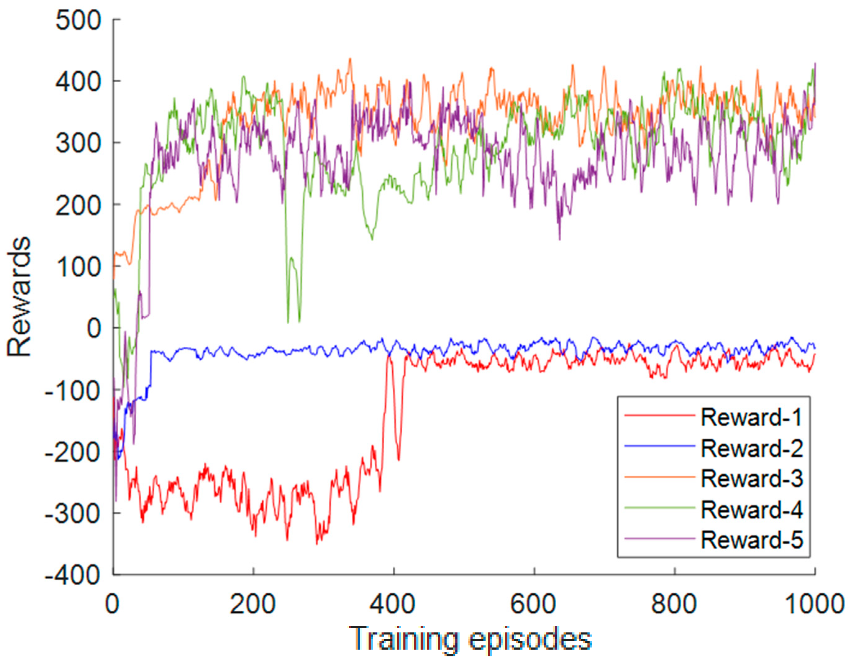
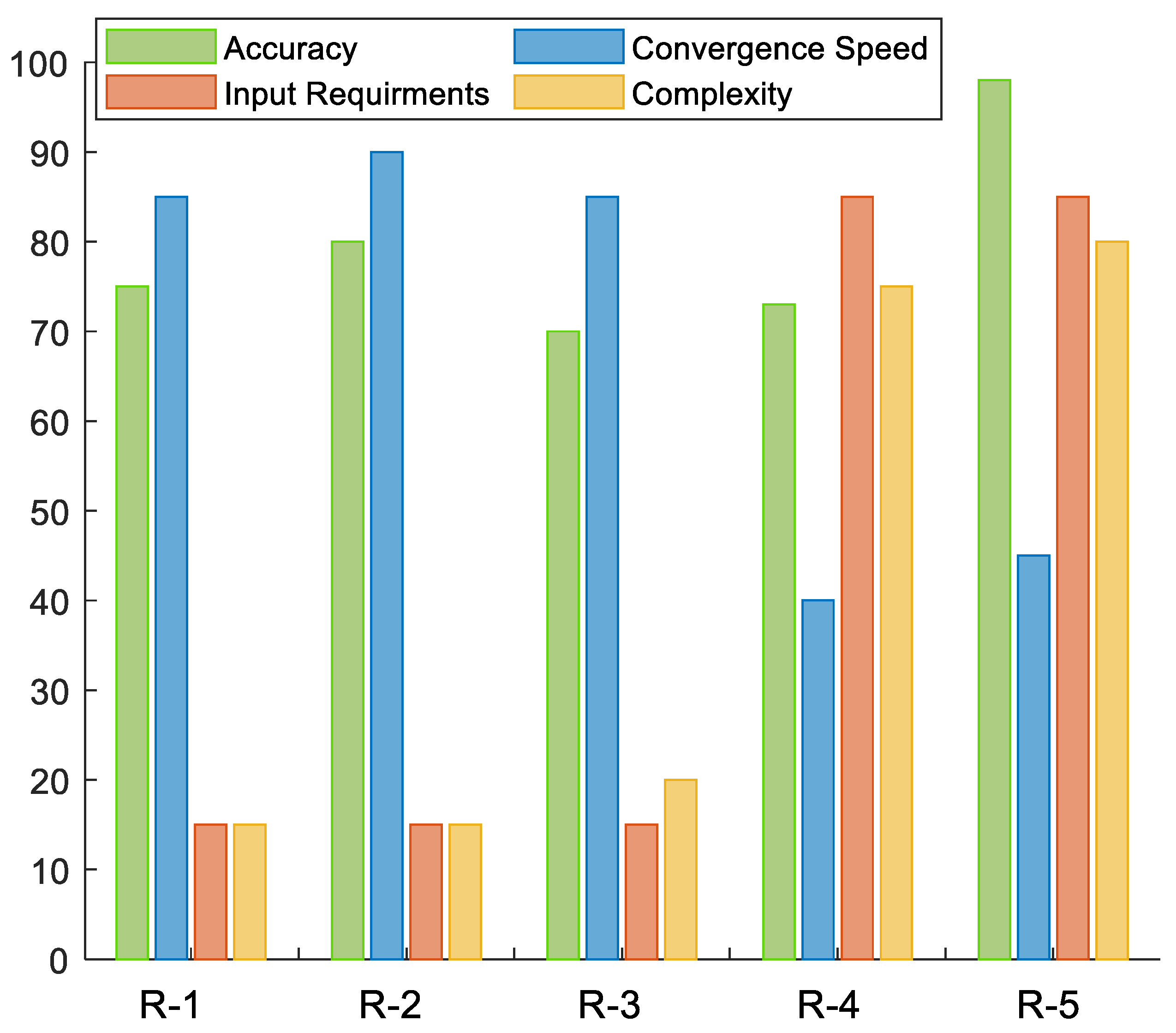
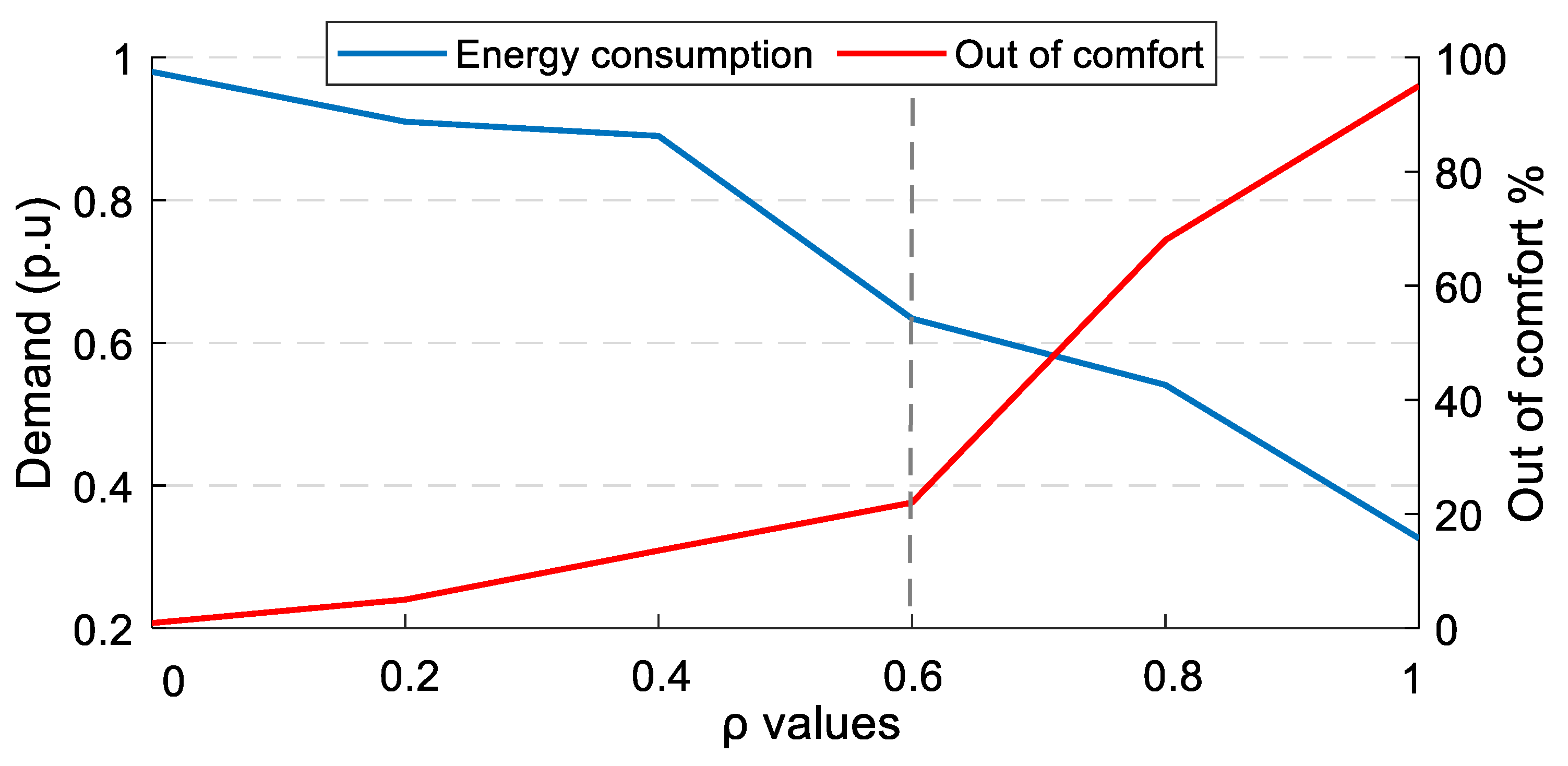
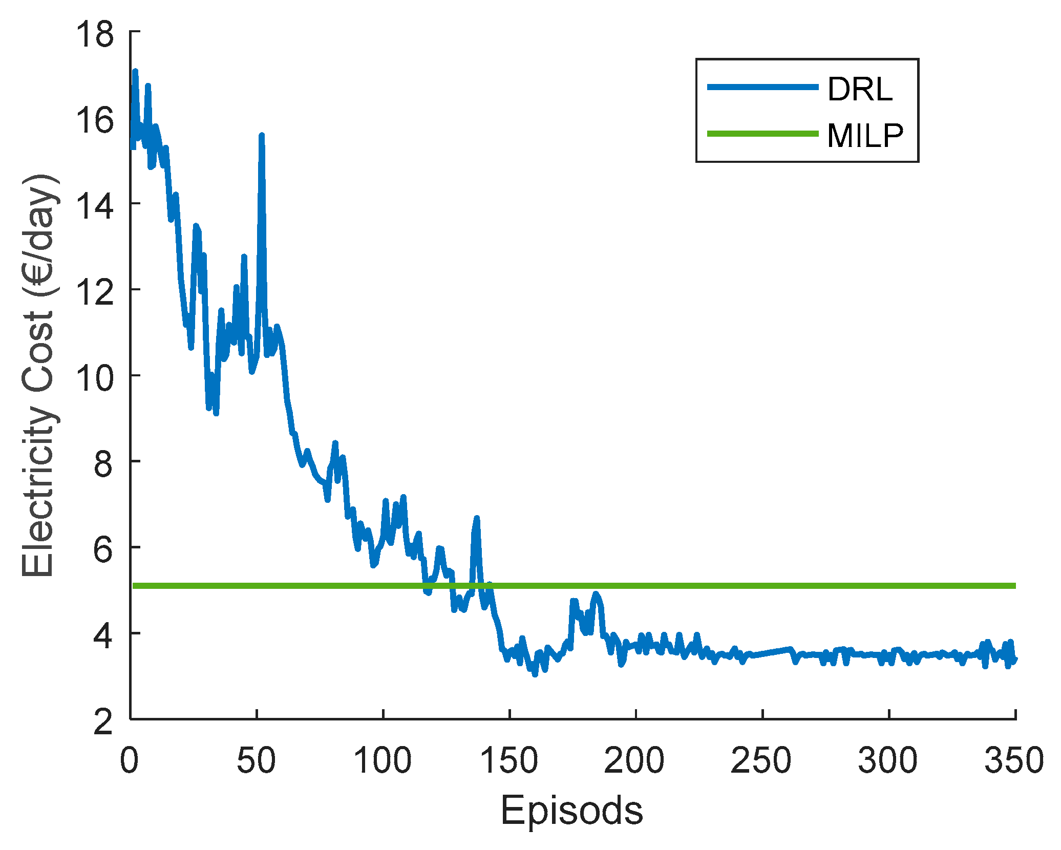
This paper addresses DRL’s technical design and implementation trade-offs for DR problems in a residential household. Recently, DRL-HEMS models have been attracting attention because of their efficient decision-making and ability to adapt to the residential user lifestyle. The performance of DRL-based HEMS models is driven by different elements, including the action–state pairs, the reward representation, and the training hyperparameters. We analyzed the impacts of these elements when using the DQN agent as the policy approximator. We developed different scenarios for each of these elements and compared the performance variations in each case. The results show that DRL can address the DR problem since it successfully minimizes electricity and discomfort costs for a single household user. It schedules from 73% to 98% of the appliances in different cases and minimizes the electricity cost by 19% to 47%. We have also reflected on different considerations usually left out of DRL-HEMS studies, for example, different reward configurations. The considered reward metrics are based on their complexity, required input variables, convergence speed, and policy robustness. The performance of the reward functions is evaluated and compared in terms of minimizing the electricity cost and the user discomfort cost. In addition, the main HEMS challenges related to environmental changes and high dimensionality are investigated. The proposed DRL-HEMS shows different performances in each scenario, taking advantage of different informative states and rewards. These results highlight the importance of choosing the model configurations as an extra variable in the DRL-HEMS application. Understanding the gaps and the limitations of different DRL-HEMS configurations is necessary to make them deployable and reliable in real environments.

This work can be extended by considering the uncertainty of appliance energy usage patterns and working time. Additionally, network fluctuations and congestion impacts should be considered when implementing the presented DRL-HEMS in real-world environments. One limitation of this work is that the discussed results only relate to the DQN agent training and do not necessarily represent the performance for other types of network, such as policy gradient methods.

References

1. Xu, C.; Liao, Z.; Li, C.; Zhou, X.; Xie, R. Review on Interpretable Machine Learning in Smart Grid. Energies 2022, 15, 4427. [Google Scholar] [CrossRef]
2. Mocanu, E.; Mocanu, D.C.; Nguyen, P.H.; Liotta, A.; Webber, M.E.; Gibescu, M.; Slootweg, J.G. On-Line Building Energy Optimization Using Deep Reinforcement Learning. IEEE Trans. Smart Grid 2019, 10, 3698–3708. [Google Scholar] [CrossRef] [Green Version]
3. Ye, Y.; Qiu, D.; Sun, M.; Papadaskalopoulos, D.; Strbac, G. Deep reinforcement learning for strategic bidding in electricity markets. IEEE Trans. Smart Grid 2019, 11, 1343–1355. [Google Scholar] [CrossRef]
4. Huang, Q.; Huang, R.; Hao, W.; Tan, J.; Fan, R.; Huang, Z. Adaptive Power System Emergency Control Using Deep Reinforcement Learning. IEEE Trans. Smart Grid 2019, 11, 1171–1182. [Google Scholar] [CrossRef] [Green Version]
5. Kwon, Y.; Kim, T.; Baek, K.; Kim, J. Multi-Objective Optimization of Home Appliances and Electric Vehicle Considering Customer’s Benefits and Offsite Shared Photovoltaic Curtailment. Energies 2020, 13, 2852. [Google Scholar] [CrossRef]
6. Amer, A.; Shaban, K.; Gaouda, A.; Massoud, A. Home Energy Management System Embedded with a Multi-Objective Demand Response Optimization Model to Benefit Customers and Operators. Energies 2021, 14, 257. [Google Scholar] [CrossRef]
7. Nwulu, N.I.; Xia, X. Optimal dispatch for a microgrid incorporating renewables and demand response. Renew. Energy 2017, 101, 16–28. [Google Scholar] [CrossRef]
8. Faia, R.; Faria, P.; Vale, Z.; Spinola, J. Demand Response Optimization Using Particle Swarm Algorithm Considering Optimum Battery Energy Storage Schedule in a Residential House. Energies 2019, 12, 1645. [Google Scholar] [CrossRef] [Green Version]
9. Dayalan, S.; Gul, S.S.; Rathinam, R.; Fernandez Savari, G.; Aleem, S.H.E.A.; Mohamed, M.A.; Ali, Z.M. Multi-Stage In-centive-Based Demand Response Using a Novel Stackelberg–Particle Swarm Optimization. Sustainability 2022, 14, 10985. [Google Scholar] [CrossRef]
10. Vázquez-Canteli, J.R.; Nagy, Z. Reinforcement learning for demand response: A review of algorithms and modeling techniques. Appl. Energy 2019, 235, 1072–1089. [Google Scholar] [CrossRef]
11. Buşoniu, L.; de Bruin, T.; Tolić, D.; Kober, J.; Palunko, I. Reinforcement learning for control: Performance, stability, and deep approximators. Annu. Rev. Control 2018, 46, 8–28. [Google Scholar] [CrossRef]
12. Wang, B.; Li, Y.; Ming, W.; Wang, S. Deep Reinforcement Learning Method for Demand Response Management of Interruptible Load. IEEE Trans. Smart Grid 2020, 11, 3146–3155. [Google Scholar] [CrossRef]
13. Mathew, A.; Roy, A.; Mathew, J. Intelligent Residential Energy Management System Using Deep Reinforcement Learning. IEEE Syst. J. 2020, 14, 5362–5372. [Google Scholar] [CrossRef]
14. Lu, R.; Hong, S.H.; Yu, M. Demand Response for Home Energy Management Using Reinforcement Learning and Artificial Neural Network. IEEE Trans. Smart Grid 2019, 10, 6629–6639. [Google Scholar] [CrossRef]
15. Xu, X.; Jia, Y.; Xu, Y.; Xu, Z.; Chai, S.; Lai, C.S. A Multi-Agent Reinforcement Learning-Based Data-Driven Method for Home Energy Management. IEEE Trans. Smart Grid 2020, 11, 3201–3211. [Google Scholar] [CrossRef] [Green Version]
16. Liu, Y.; Zhang, D.; Gooi, H.B. Optimization strategy based on deep reinforcement learning for home energy management. CSEE J. Power Energy Syst. 2020, 6, 572–582. [Google Scholar]
17. Amer, A.; Shaban, K.; Massoud, A. DRL-HEMS: Deep Reinforcement Learning Agent for Demand Response in Home Energy Management Systems Considering Customers and Operators Perspectives. IEEE Trans. Smart Grid 2022. [Google Scholar] [CrossRef]
18. Li, H.; Wan, Z.; He, H. Real-Time Residential Demand Response. IEEE Trans. Smart Grid 2020, 11, 4144–4154. [Google Scholar] [CrossRef]
19. Ye, Y.; Qiu, D.; Wang, H.; Tang, Y.; Strbac, G. Real-Time Autonomous Residential Demand Response Management Based on Twin Delayed Deep Deterministic Policy Gradient Learning. Energies 2021, 14, 531. [Google Scholar] [CrossRef]
20. Huang, C.; Zhang, H.; Wang, L.; Luo, X.; Song, Y. Mixed Deep Reinforcement Learning Considering Discrete-continuous Hybrid Action Space for Smart Home Energy Management. J. Mod. Power Syst. Clean Energy 2020, 10, 743–754. [Google Scholar] [CrossRef]
21. Ahrarinouri, M.; Rastegar, M.; Seifi, A.R. Multiagent Reinforcement Learning for Energy Management in Residential Buildings. IEEE Trans. Ind. Inform. 2021, 17, 659–666. [Google Scholar] [CrossRef]
22. Yu, L.; Xie, W.; Xie, D.; Zou, Y.; Zhang, D.; Sun, Z.; Zhang, L.; Zhang, Y.; Jiang, T. Deep Reinforcement Learning for Smart Home Energy Management. IEEE Internet Things J. 2020, 7, 2751–2762. [Google Scholar] [CrossRef] [Green Version]
23. Ruelens, F.; Claessens, B.J.; Vandael, S.; De Schutter, B.; Babuška, R.; Belmans, R. Residential Demand Response of Ther-mostatically Controlled Loads Using Batch Reinforcement Learning. IEEE Trans. Smart Grid 2017, 8, 2149–2159. [Google Scholar] [CrossRef] [Green Version]
24. Lee, S.; Choi, D.H. Reinforcement learning-based energy management of smart home with rooftop solar photovoltaic system Energy Storage System, and Home Appliances. Sensors 2019, 19, 3937. [Google Scholar] [CrossRef] [PubMed] [Green Version]
25. Honarmand, M.; Zakariazadeh, A.; Jadid, S. Optimal scheduling of electric vehicles in an intelligent parking lot considering vehicle-to-grid concept and battery condition. Energy 2014, 65, 572–579. [Google Scholar] [CrossRef]
26. Paraskevas, A.; Aletras, D.; Chrysopoulos, A.; Marinopoulos, A.; Doukas, D.I. Optimal Management for EV Charging Stations: A Win–Win Strategy for Different Stakeholders Using Constrained Deep Q-Learning. Energies 2022, 15, 2323. [Google Scholar] [CrossRef]
27. Mosavi, A.; Salimi, M.; Ardabili, S.F.; Rabczuk, T.; Shamshirband, S.; Varkonyi-Koczy, A.R. State of the Art of Machine Learning Models in Energy Systems, a Systematic Review. Energies 2019, 12, 1301. [Google Scholar] [CrossRef]
Figure 1. HEMS interfacing with different types of household appliances and assets.
Energies 15 08235 g001
Figure 2. Agent and environment interaction in RL.
Energies 15 08235 g002
Figure 3. The general architecture of DRL.
Energies 15 08235 g003
Figure 4. DRL-HEMS structure.
Energies 15 08235 g004
Figure 5. DQN agent implementation flowchart.
Energies 15 08235 g005
Figure 6. The differences between the training dataset, validation dataset, and testing dataset.
Energies 15 08235 g006
Figure 7. Learning steps and % of scheduled appliances using different learning rates.
Energies 15 08235 g007
Figure 8. Reward function for different exploration rates.
Energies 15 08235 g008
Figure 9. Reward functions for different scenarios.
Energies 15 08235 g009
Figure 10. Bar chart of the trade-offs for each reward configuration.
Energies 15 08235 g010
Figure 11. Comfort and energy-saving trade-offs.
Energies 15 08235 g011
Figure 12. Total electricity costs over one day by DRL agent and MILP solver.
Energies 15 08235 g012