Article

Application of Artificial Intelligence in the Unit Commitment System in the Application of Energy Sustainability

Faculty of Civil Engineering, Czech Technical University, 166 29 Prague, Czech Republic
Energies 2022, 15(9), 2981; https://doi.org/10.3390/en15092981
Submission received: 4 March 2022 / Revised: 4 April 2022 / Accepted: 14 April 2022 / Published: 19 April 2022
(This article belongs to the Special Issue Smart Grid Control and Optimization)

Abstract

:
This article approaches the optimal solution of energy sustainability based on the use of artificial intelligence (AI). The application of renewable energy sources (RES) and unit commitment (UC) is the basic idea of this concept. Therefore, a new approach to solving the UC problem is introduced. The proposed method has a simple procedure to obtain the popular solutions in an acceptable time interval, by creating a basic model of the schedule of the state of energy units RES. It is obvious that individual consumer units, of an operational nature, take hourly performance values by performing economic evaluations on them in the sense of cost optimization. This is conducted through an artificial intelligence (AI) algorithm by optimizing the dedicated cost function, simulated by annealing. Despite the acceptable solution obtained from these two steps, another shift is proposed, called the TDD process in a given consumer area. This process in the application of AI in the system of selection of universal load TDD from hundreds of possible ones is based on the use of artificial neural networks and cluster analysis, which is represented by the application of the Kohonen map. This logical process to achieve a modified solution is a self-organizing map (SOM). It is a software tool for visualizing high-dimensional data. Converts complex, nonlinear statistical relationships (functions) between high-dimensional data to simple geometric relationships, low-dimensional representation. The output of SOM is an optimized load TDD on the basis of which the process of automatic control of UC in the local urban area is built. The results of the AI application in the case of sustainable energy solutions confirm that this UC method provides a robust solution to an almost optimal solution.

1. Introduction

A smart city should be pleasant for its inhabitants to live in. This process already arises at the level of its individual compact districts (cities, clusters of buildings and buildings as such), streets, housing estates and individual housing in houses and flats. Today’s current situation is accepted on the platform of requirements for the construction of NZEB (Nearly zero-energy buildings), which is based on the directive of the European Parliament. It requires that new construction projects be nearly zero energy buildings from 1 January 2020. This state of construction and execution of NZEB is described in detail in a number of articles, communications, decrees and laws (in all countries of Europe and the world), which are commonly known. The basis is that such buildings must meet the conditions that the primary energy consumption per year is (50 to 70) kWh/m2 of usable area of the apartment and the coverage from RES per year is 30 kWh/m2 of usable area of the apartment. In this concept, we are talking about tz energy efficiency or building efficiently and choosing energy efficient construction. In fact, these new buildings will be only 10 to 20% more economical compared to the apartment buildings built so far.
In the context of a compact city (compact neighborhoods), the following topics are addressed: reducing growing car traffic in cities; reducing emissions and air pollution; revitalization and reuse of urban brownfields; development of public transport; or the so-called smart growth of the city with a focus on energy savings. This led to the choice of research focus within the experiment on the most current topic, namely:
  • Energy savings (electricity).
  • Reduction of CO2 emissions and air pollution.
It should be emphasized that energy is directly linked to the competitiveness of countries, as it is the key to sustainable development, i.e., where energy production and consumption have the greatest impact on the environment in terms of climate change and air pollution [1]. On the other hand, energy is the main engine of economic growth. Based on the analysis, sustainable energy development can be achieved by separating gross domestic product (GDP) from energy consumption and by separating energy consumption from air pollution, including greenhouse gas emissions [2,3]. In the above focus, this research further focused on improving:
  • Energy efficiency, i.e., decoupling economic growth from energy consumption.
  • Increased use of renewable energy sources (RES); which makes it possible to separate energy consumption from greenhouse gas emissions; which should be kept to a minimum.
Research rationale:
Both approaches address energy efficiency and the use of RES, which are seen as policies to promote sustainable energy and the competitiveness of developing countries [4,5,6,7]. If there are policy approaches to promote sustainable energy development, then sustainable energy indicators can be used to determine how to define the boundaries and framework for sustainable energy development. These indicators make it easier to assess different sections of sustainability and compare the progress of different countries towards sustainability over the years [8].
Energy savings are then the amount of energy saved, determined by measuring or estimating consumption before and after the implementation of one or more energy efficiency measures under standardized external conditions that affect energy consumption. Increased energy end-use efficiency will also reduce primary energy consumption, reduce CO2 and other greenhouse gas emissions, and thus prevent dangerous climate change. Increasing energy end-use efficiency will allow the potential for investment-efficient energy savings to be realized in an economically viable way. Energy efficiency measures lead to energy savings that help reduce countries’ dependence on energy imports. The use of more energy efficient technologies increases the pressure to introduce new innovative technologies and the competitiveness of the economy.
The contribution and novelty of this research is:
  • Focus on fulfilling energy sustainability and optimizing the performance balance of compact urban neighborhoods (clusters of buildings).
  • Unit Commitment (UC) application, which is the process of deciding when and which sources of electricity, for example, in our case the local micro-network of RES, start and stop. This is an important task in the operation of the electricity system and the local island system. This is a system demand in a short period of time. On the other hand, such a restructured system can ensure the supply of electricity, for example, to a city district or city, and can be competitive while allowing consumers to choose an electricity supplier. UC systems are also characterized by sufficient storage and time-consuming calculations. The UC structure has in the past been defined as a schedule of production units to be in operation (on/off) in order to minimize total production costs while meeting all constraints, such as power consumption, minimum on and off time, etc. On the other hand, UC in Deregulatory environments is more complex and competitive than traditional UCs. Such models have been developed by examining the effects of the dynamic growth of electricity produced in the intermittent renewable energy target (RET) system [9]. In a previous study [10], an optimization method was proposed, which addressed the system of dynamic economic management of individual residential loads and charging stations for electric vehicles. In part, our test system has shown that shifting load-bearing loads can significantly flatten the load profile and reduce peaks.
The rationale for the benefits, and therefore, the novelty, of this research, lies in the following communication:
  • It is based on the amendment to Directive 2010/31/EU on energy performance in the part of definitions and interpretations of terms. The term “technical building system” includes technical equipment for heating, cooling, ventilation, domestic water heating, built-in lighting, building automation and control, on-site electricity generation, or a combination thereof, including systems using renewable energy from the building or building unit. The definition of a technical system is, therefore, extended to include local electricity generation and automation and control systems, which are further defined as systems consisting of all products, software and engineering services that provide automatic control or facilitate manual operation.
  • A major transformation is currently underway to reduce climate change, energy consumption and CO2 emissions. Another important stage of energy infrastructure is to achieve carbon neutrality for the Czech Republic (CR) in electricity generation by 2050. It is about ensuring the replacement of brown coal in the Czech heating industry by 2030 and 2040 at the latest, using alternative energy sources, especially photovoltaic systems. Energy is one of the most affected sectors. The sector now faces many new challenges, including greater use of flexibility from smaller sources, especially RES. As for the flexibility itself, it can be used to ensure energy balance in the system (micro-RES networks), energy trade, or manage its own fluctuations.
The aim of the research work:
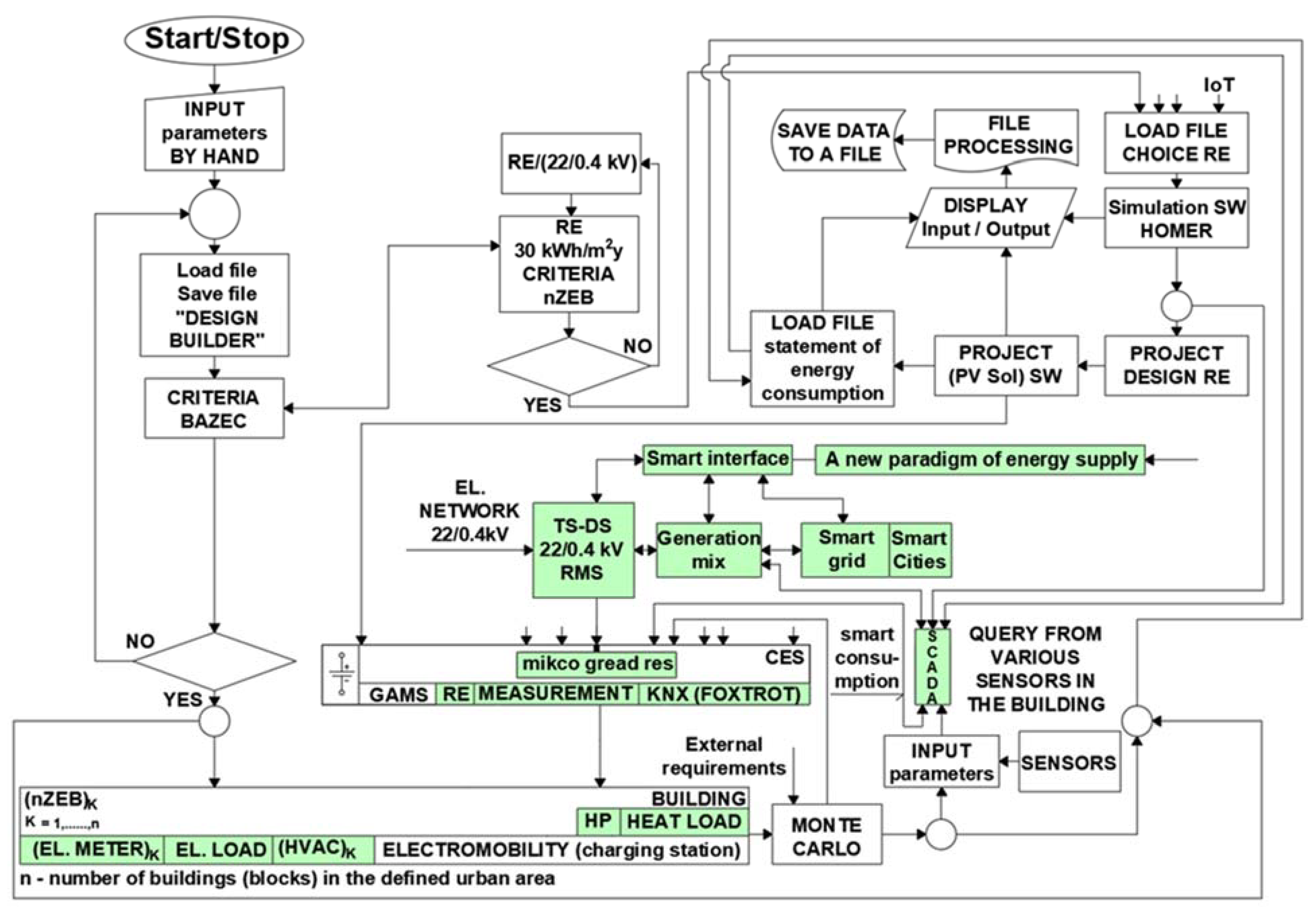
  • Design of a micro-network of RES with decentralization of sustainable energy in a defined urban area (cluster of buildings) with the application of an artificial intelligence automated unit commitment (UC) system on the RES platform to optimize power balance (balancing the immediate deviation between production and consumption).

2. Materials and Methods

When modelling the RES-based energy systems installed on the building roofs in the Prague-Bubeneč district using the HOMER (Hybrid Optimization Model for Electrical Renewable) software, the results show that the design of the RES system is very efficient within a 1000 m building cluster [11] This conclusion can be considered crucial because it is the result of a larger number of simulations in our experiment.
Why build a building cluster
The transition from centralised to decentralised electric power generation requires and stimulates a large amount of research in a wide range of areas: Distributed Sources and Infrastructures; Energy Efficiency Renovation; RES Solutions; Distributed Generation Performance; Energy Storage Behaviour and Economics; Demand Side Management and Virtual Power Plants; Microdevices, Energy Devices and Plug-in Vehicles; Growing ICT Penetration; Artificial Intelligence and Data-Driven Governance [12].
Simulation of Energy Performance of Buildings (EPB) at the scale of a single building is not accurate enough to respond to the urban energy system. The building cluster represents a possible intermediate benchmark for a detailed assessment of the interaction between buildings and urban energy infrastructures while taking into account current computing capacity and intelligence. Figure 1 interprets the ongoing transformation of buildings into cluster-defined units.
Space-time dimension of a building cluster
A spatial scale is used to describe the size of the building cluster area for energy planning/simulation purposes. The building cluster’s factors in terms of EPB include the energy grid, RES electric power generation, and the building. Among them, there are factors influencing the energy performance of the cluster: building envelope design, RES design, solar energy potential, building density, energy demand, integrated systems and energy hub (energy centre).

2.1. RES Unit Commitment to Optimize the Performance Balance

In terms of energy savings in buildings, it motivates energy companies to plan energy production (in this case, electric power) according to demand (consumption) as economically as possible. By optimally distributing the electric power generation among the various units, a significant amount of fuel and costs on production thereof can be saved. In other words, it is important to determine whether the unit must be on/off. It is talking about the so-called Unit Commitment (UC). It is a fundamental problem of economic optimization in energy systems.
The UC problem becomes increasingly complex with the RES integration in a defined cluster of buildings (urban district) due to differences in behaviour and functional limitations with respect to conventional thermal units that need to be addressed as renewable generation shall be an integral part of the smart grid.

2.1.1. Unit Commitment Problem in the RES Energy System

This study aims to address the energy performance of buildings in order to reduce energy consumption and CO2 production. The building energy model (BEM) was designed, including the implementation of a smart micro RES network; see Figure 2 [13]. The problem of a balanced energy balance has been solved. It is normally solved using frequency and active power control in case of power balance disturbance due to practical reasons on the consumer side.
Now, there is the problem of unit commitment (UC) in the presented energy system consisting of a RES microgrid within the presented experiment of the urban area of Prague 6. Addressing the issue of UC application is important primarily because of other measures aimed at reducing energy consumption and, thus, CO2 emissions. This problem is outlined by solving the UC special-purpose (objective) function, which can be formulated as the sum of the costs of all units (sub-units of photovoltaic power plants) over time, expressed mathematically as [14,15]:
F = t = 1 T i = 1 N [ ( u i ( t ) F i ( t ) ) + S i ( t ) ]
The constraint models for the UC optimization problem are as follows.
  • Energy balance of the system
i = 1 N [ u i ( t ) P g i ( t ) + u i ( t 1 ) P g i ( t 1 ) ] = P D ( t )
  • Energy and power exchange
E i ( t ) = [ P g i ( t ) + P g i ( t 1 ) ]
  • Backup requirements
i = 1 N u i ( t ) P g i ( t ) P D ( t ) + P R ( t )
  • Energy generation limits of given units (RES)
P g i m i n P g i ( t ) P g i m a x
At t { 1 ,   T } and i { 1 ,   N } in all cases where:
  • F : Total operating costs of the energy system
  • E i ( t ) : Output energy from the i-th unit in t hours
  • F i ( E i ( t ) ) : Fuel cost of the i-th unit in t hours
  • u i ( t ) : Power generation ratio and its capability
  • N : Total number of units in the system
  • T : The total time for which UC is performed
  • P g i ( t ) : Output of the i-th unit in an hour of t
  • P g i m a x : Maximum output power of the i-th unit
  • P g i m i n : Minimum output power of the i-th unit
  • S i ( t ) : Initial cost of the i-th unit in t hours
Lagrangian relaxation is commonly used to solve UC problems. It is much more beneficial for the functionality of a RES microgrid having many units, as the degree of partial optimality decreases towards zero as the number of units increases. The model characteristics of specific units are easier to modify, and constraints for those units are relatively easy to add. The drawback of Lagrangian relaxation [16] is its inherent partial optimality.
L ( λ ,   μ ,   ν ) = t = 1 T i = 1 N [ C i ( P g i ( t ) ) + S i ( x i ( t ) ) ] + λ ( t ) ( P d ( t ) + P R ( t ) P g i ) + μ ( t ) ( P g i m a x P g i )
where λ ( t ) ,   μ ( t ) are the multipliers associated with the requirement for time t.
A solution approach using a variant of ADP (Adaptive Dynamic Programming) for the UC problem: ADP is able to optimize the system over time under conditions of noise and uncertainty. Suppose optimal operation patterns are used to train (learn) the neural network from ADP. In that case, the neural network can learn how to arrange or adapt generators according to the operator’s patterns and change the mode of operation according to load changes.
In addition to the application of the building energy model (BEM) in connection with the NZEB solution, there is the issue of energy savings, its safety, reliability and quality at a given time. The RES-based platform plays a very important role. We are talking about the so-called micro-networks of RES in the system of parallel operation, as their local aggregation on the roofs of buildings of individual residential zones A, B, C, D, E and F, see Figure 3.
This will create six independently operating RES units in parallel operation with a common backup and a connected distribution network of 22/0.4 kV. The steady operation of the microgrid is ensured by a partial supply of electricity from the distribution network and battery storage. The optimization of eclectic energy consumption is then ensured by the unit commitment of RES.
The unit commitment plan for RES and their generated electricity outputs covers the predicted consumption for each hour within one day. We used an artificial neural network (UNN), a fuzzy model structure and cluster analysis as methods of artificial intelligence (AI) to evaluate the necessary data. We will create several types of daily consumption in graphical form, which will then be grouped into so-called clusters. The output will then be two objects of the same cluster similar to two objects of different clusters. The result will be so-called prototypes. Subsequently, prototypes, cost factors and constraints will be considered as inputs for UNN.

2.1.2. Teoretika Assumptions for Slovník the Unit Commitment of Our Experiment

UC is a computational process of economic handling, where the total required generation of electricity from RES is distributed among multiple loads (complete units) of operation while minimizing the selected cost criterion [17], conditioned by loads and operating constraints.
For each load condition, the power from each electrical device is calculated, which actually minimizes the total cost of input primary energy needed to run the load [18]. Traditionally, this function is formulated as a cost optimization, which we express as a quadratic function [19]:
f ( P ( t ) ) = i = 1 N ( i + β i P i ( t ) + γ i P i 2 ( t ) ) ,
f ( P ( t ) ,   x ( t ) ) = f ( P ) · x i ( t ) ,
i = 1 N P i i = 1 N D P D i + P z T = 0 .
where
  • N —total output of the RES microgrid
  • N D —total power consumed
  • P Z T —total power loss
  • x i ( t ) —power of the i-th source of RES at time t
  • P i ( t ) —output power of RES microgrid
  • P D i —power consumed
  • P —nominal power of RES, where the variable P is expressed as Pi
  • P i —is the output power of the i-th RES (i = 1 to 8; we have a total of 6 sources of photovoltaic systems FV1 to FV6 located on the residential units A, B, C, D, E and F, as well as cogeneration and substation TS-DS) in time t
  • x i ( t ) —power state of the i-th source at time t
  • i ,   β i ,   γ i   and   i ( t ) —cost coefficients (downtime) and time constant exp. the increase in the initial costs of the i-th source at time t
  • i [ CZK ] —costs depending on the output produced, β i [ CZK / W ] —costs dependent on heat loss (Joule heat), a γ i [ CZK / W 2 ) ] —costs caused by iron losses and friction.
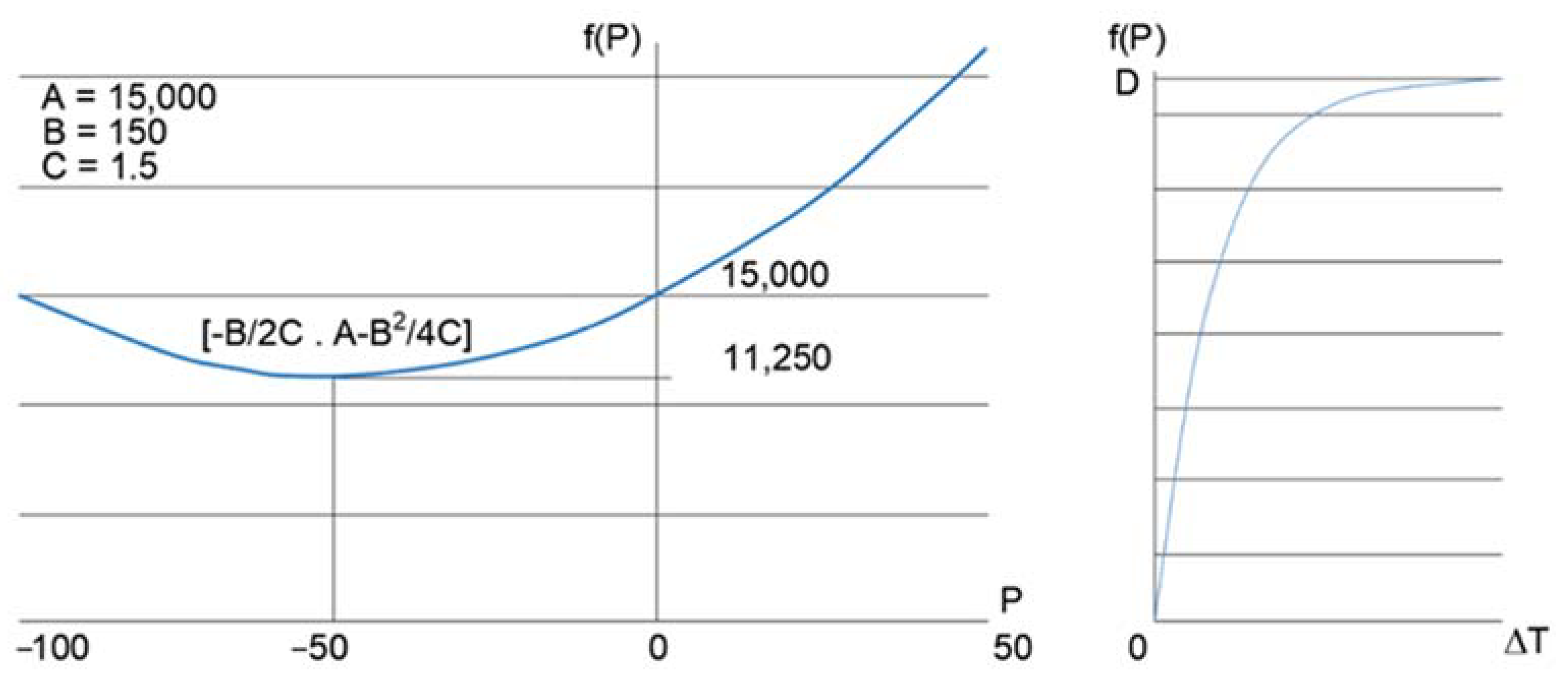
    V m i n V V m a x ,
    P i m i n P i P i m a x
From relations (10) and (11) it is evident that P i m i n and P i m a x is the minimum and maximum electrical power of the local RES microgrid. Subsequently, V ,   V m i n   and   V m a x , is the voltage obtained from the RES microgrid and the minimum and maximum voltages of this network are closely related to this. It follows from the mentioned relations (10) and (11), which express certain limitations or limit values of voltage and power parameters, that are suitable for their analysis and application in the interest of energy optimization to use some mathematical programs. These are, for example, linear or nonlinear programming, quadratic programming and other methods. Subsequently, we recommend using alternative solution methods, such as evolutionary programming (EP) [17], genetic algorithms (GA) [20], taboo search [21], neural networks [22], particle swarm optimization [23,24] and adaptive dynamic programming (ADP). Through this process, when applying artificial intelligence methods, we achieve the necessary improvement in the performance of the economic manipulation algorithm. Therefore, we express the optimization problem according to [15] as follows:
f : n   f ( x 0 ) = min x f ( x )   n
where Ω represents the area of accessible solutions, taken from the point of view of the operational and technical parameters of RES and x 0 is the optimum of the function f being sought. The function f is a cost or criterion function, Figure 4, for electricity in a defined period, we also start from the idea see [15].
Figure 4. Dependence of operating costs on energy and downtime. Note: f(P)—Start-up costs; ΔT—Downtime; P—Operating costs.
Energies 15 02981 g004
f ( P ( t ) , x ( t ) ) = t i ( i + β i P i ( t ) + γ i P i 2 ( t ) + δ i ( 1 e Δ T i ( t ) τ i ) )   x i ( t )
f ( x ( t ) ) = t i ( i P i + β i P i 2 ) x i ( t ) + γ i x i ( t ) ( 1 x i ( t 1 ) )
We will proceed from the relation (14) of the purpose function, where:
(a)
The first sum in relation (14) ( i P i + β i P i 2 ) x i ( t ) , expresses operating costs.
(b)
The second summand in relation (14) γ i x i ( t ) ( 1 x i ( t 1 ) ) , expresses the so-called start-up costs.
Note: i ,   β i ,   u n d   γ i are cost coefficients resp. downtime.
It should be emphasized that the operating and start-up costs of RES within the RES microgrid are integrated over a given period of time.
The cost function (14) has its accessible solutions and these are determined by certain conditions, which are based on our experiment. If we look at an acceptable solution of the purpose (cost) function, then we can define the following equations or inequalities:
i P i x i ( t ) = C ( t )
P i m i n P i P i m a x
For t = 1.2, …, 24 h.
From relation (15) it is clear that it defines the state of the source (RES) always at a given hour. In our case, it is the sum of the power of the switched-on sources within the RES microgrid. The whole process depends on the state of resources in a given hour, which can be expressed by the relation x ¯ ( t ) = ( x 1 ( t ) ,   x 2 ( t ) , ,   X 10 ( t ) .
By adjusting the above relationships, we obtain the relationship for another limiting condition of the cost function, and that is:
g ( x ( t ) ) = i P i x i ( t ) C ( t ) = 0
The minor in the form P i x i ( t ) expresses in our case the produced electric energy in part t and the minor in the form C ( t ) predicts the electricity consumption in a given hour. P i is the output electrical emergence from RES, P i m i n is the minimum output electrical energy from RES and P i m a x is the maximum output electrical energy from RES.
Equation (16) means that we produce such an amount of electricity at a given time that electricity is also consumed at that time. Mathematically, this means that the predicted electricity consumption at a given time in the considered period of the year approaches as much electricity as possible in the same period.
Where x i ( t ) expresses the state of the i-th source at time t (the state on indicates the number l o g   1 and the state off indicates the number log 0), it is a binary expression. Furthermore, i { 1 ,   2 ,   ,   N } , where i is the source index and N expresses the number of sources in the microgrid, which in our case is 10 (ten words). Furthermore, t { 1 ,   2 ,   ,   T } expresses the time of the planned unit commitment regime in the microgrid and T is 24 h (day). Furthermore, P i ( t ) expresses the power of the i-th source at time t and P i is considered in our case as P i ( t ) .
The purpose function has independent variables ( x 1 ,   x 2 ,   ,   x n ) , where n = 10 number of electricity sources. The status of each electricity source is either “0”—generator off or “1”—generator on. Where ( x 1   a ž   x n ) —are the components of the vector. We will now explain the meaning of a mathematical expression
  x i ( t ) ( 1 x i ( t 1 )
Figure 5 shows a pictorial representation of the mathematical expression (15), which indicates the predicted time when the demand for electric power to power the appliances occurs or does not occur, i.e., the power sources are started up.
Conclusion: In the first hour: γ i x i ( t ) ( 1 x i ( t 1 ) . γ i · 0 = 0 →running costs are zero.
In the second hour, start-up costs γ i are also zero. In the third hour, the financial value of the start-up costs is taken into calculation.
There is always an effort to keep the cost (objective) function as small as possible.
The cost function is divided into:
(a)
  ( i P i + β i P i 2 ) x i ( t ) operating costs
(b)
  γ i x i ( t ) ( 1 x i ( t 1 ) start-up costs
The coefficients in the cost function (14) are expressed in units, such as: i   [ CZK ] ,   β i [ CZK MW ]   a   γ i   [ CZK M W 2 ] .
When using relation (15), which is a constraint of the purpose function and when including it in this purpose function fg, we obtain the relations (19) and (20)
f g ( x ) = f ( x ) + w   g 2 ( x ) m i n .
f g ( x ) = f ( x ) w   μ ( g ( x ) )
We have previously designated the purpose function as f ( x ) , then w g 2 ( x ) will express in relation (19), the unsolicited supply of electricity, which we will consider as a sanction of unsolicited supply. Furthermore, the value w of the function g 2 ( x ) defines the conditions of the purpose function. The μ parameter indicates the fuzzy number zero.
Next, we will consider the association function of the fuzzy number zero Figure 6.
μ ( g ( x ) ) = ( Δ P   | g ( x ) | ) / Δ P   g ( x ) Δ P , Δ P
μ ( g ( x ) ) = 0   g ( x ) Δ P , Δ P
where w is the weight of state (19) and (20);
  • μ 
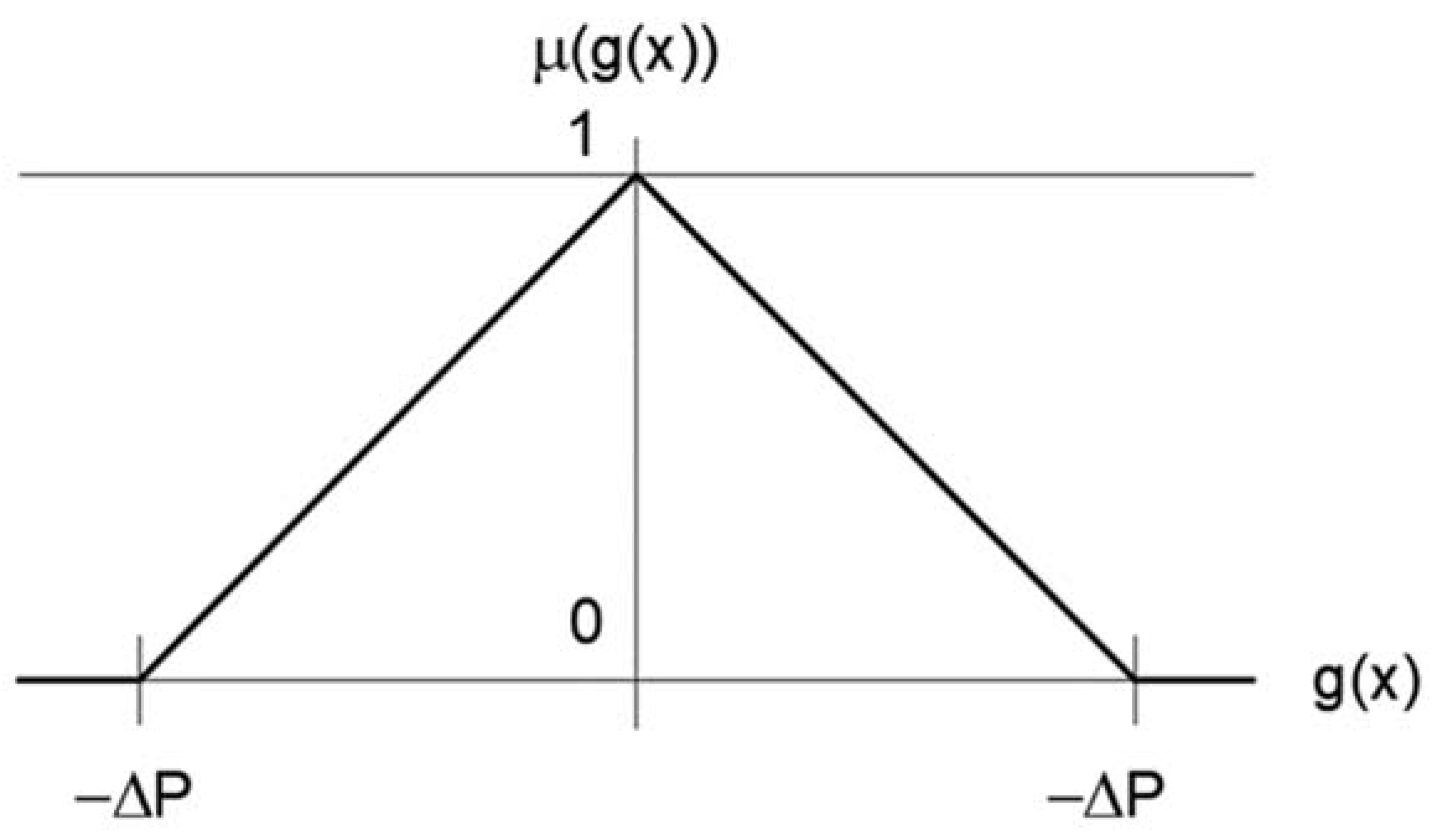
is the fuzzy number zero Figure 6;
  • Δ P is the maximum permissible tolerance for the balance.
Figure 6. Fuzzy number affiliation function.
Energies 15 02981 g006
Note in Figure 6: The allowable solution ranges from −∆P to ∆P. It is always an attempt to make a solution to the environment acceptable, e.g., zero; then in that case the limiting condition will be satisfied, i.e., μ ( g ( x ) ) = 1 . If Δ P = 0 , then the constraint is fully satisfied.

2.2. Application of the Simulated Annealing Algorithm in Our Experiment

Practical problems never lead to simple problems, it is often difficult or impossible to find a plausible mathematical description or algorithm to solve such a problem. In some cases, it is possible to find an exact mathematical description, but on the other hand, their exact solution is not possible with current computer technology to achieve the expected results in real time. Therefore, a number of heuristic methods have been developed that often do not find an exact solution to a given problem in terms of optimality. The problem that the work deals with was solved based on heuristic methods. Various techniques were used to find the optimal schedule, and in our research, we compared some in terms of solving the problem of optimizing energy systems. This article is dominated by the simulated annealing optimization method as one of the heuristic methods we have applied. The simulated annealing (SA) method has the most stochasticity. The method adopts a worse solution based on a certain probability (given by the Metropolis criterion).
The inspiration of the SA method is the physical process of annealing a solid body, in which defects of the crystal lattice are removed. The starting point of the physical process is a process that is based on the similarities between the process of annealing a solid material and general combinatorial optimization [25]. The search process is based on a random event. When iterating to update a feasible solution, a solution worse than the current solution is likely to be accepted, so that it is possible to obtain an optimal global solution by jumping from a locally optimal solution [26]. As mentioned in [27,28,29], the SA algorithm has been improved to some extent through some combination with other algorithms. This resulted in better results in the experiments performed. We also confirmed this fact in our experiment. An example of this conclusion is given in Figure 7.
It can be seen from Figure 7 that the default solution is the left blue dot A. The SA algorithm quickly finds the optimal local solution B (local optimum), but after finding the local optimum, the solution does not end there but moves on to the next one with a certain probability. Probably after several non-locally optimal moves, the global optimum D is reached and a jump to the local minimum.
The mathematical expression is based on the principle of thermodynamics, where at temperature T there is a probability of temperature decrease with the difference of energies d E and p ( d E ) , which is expressed as:
p ( d E ) = exp ( d E k T ) ,
In relation (23) the individual parameters are expressed such that k is a Boltzmann constant having a value of 1.3806488 × 10 23 and d E < 0 . Therefore, d E k T < 0 , it follows that the range of values of the function p ( d E ) is ( 0 ,   1 ) . If we look at the above formula without long rational consideration, then: the higher the temperature, the greater the probability that the energy difference is expressed by the notation p ( d E ) , and the lower the temperature, the lower the probability of a decrease in temperature.
In practical problems, the calculation of a “certain probability” here relates to the process of annealing metal melting. Assuming that the currently feasible solution is x n e w , and the iteratively updated solution is xne, then the corresponding “energy difference” is defined as:
Δ f = f ( x n e w ) f ( x ) ,
and consequently, the corresponding certain probability is expressed by the relation:
p ( Δ f ) = ( 1 , i f Δ f > 0 exp ( Δ f k T ) , i f Δ f 0 )
We start from the initial value k = 1 . The SA algorithm is described as follows:
Step 1: Setting initial values: Initial temperature T (large enough), original best solution x obtained after GA (genetic algorithm) [30,31] used; solution obtained from the previous iteration xnew.
Step 2: Now we calculate the increment Δ f = f ( x n e w ) f ( x ) , where f ( x ) is the goal of optimization. Basically, it is a function that minimizes the mean absolute error ϵ and is calculated according to the sampling. We use the result one minus ϵ , which represents the value of the fitness function.
Step 3: For the case when Δ f > 0 , xnew is accepted as the new current solution, then xnew is accepted as the new current solution with probability exp ( Δ f k T ) .
Step 4: If the termination condition is met, the output is another current solution as the optimal solution for terminating the program. If this does not happen, we will wait for the new x n e w and go to step 2.
We will also mention the situation when we choose temperature reduction as an exponential function, for example:
T = T 0 e i t e r τ   τ = N ln T T 0   T lim i t e r T 0 e i t e r τ = 0
where: T is temperature decreases exponentially during the iteration cycle (also expresses that no better solution will be provided because a worse solution can be accepted to some extent); T 0 is the initial temperature; T is the final temperature; τ is the time constant; N is the number of iterations.
Many problems in engineering, planning and manufacturing can be modeled as that of minimizing or maximizing a cost function over a finite set of discrete variables. That is the problem with this research. Simulated annealing is one of the best known local search algorithms because it works quite well and is widely used. The algorithm and flowchart of simulated annealing are presented in [32].
The simulated annealing procedure is based on simulating the physical processes taking place during the removal of crystal lattice defects. There is a simple algorithm called the Metropolis algorithm (1953 N. Metropolis), working on the principle of the Monte Carlo method: We start from the moment when the current state of the system is determined by the position of the particles of the body. Subsequently, the particles are gently shifted, causing a small random symmetric fault (i.e., the probability of a change of state A to state B due to the fault must be the same as the change of state B to A). We state that faults are generated until the energy difference between the current and the disturbed state 4E is non-negative. Then, the probability of accepting the violated state into the next process is determined by the relationship P r = m i n ( 1 ,   e ( Δ E ) k T ) . Where T is the Boltzmann constant, and Δ E is the difference between the energies of the current and disturbed state.
It is this acceptance of the disturbed state that we call the Metropolis criterion. Algorithm 1 shows us the principle of the Metropolis algorithm, written in PYTHON.
The heuristic simulated annealing (SA) method will be used to solve this problem. The SA principle can be seen in Figure 6 and Algorithm 1 written in the PYTHON language is part of the program for optimizing the target (cost) function of the presented experiment.
Algorithm 1. Procedure Metropolis algorithm.
Input:  x i n i ,   k m a x ,   T ,
  o u t p u t :   x o u t ;
#Metropolis Algoritmus
def MetropolisAlgorithm(xini, kmax, t):
  self.k = 0
  self.x = xini
  while self.k < kmax
    self.k++
    self.xt = Opert(self.x)
    self.pr = min(1, exp(−(f(self.xt) − f(self.x))/t))
    if random() < self.pr:
      self.x = self.xt
  return self.x
In the algorithm, x i n i indicates the initial state, k m a x is the maximum number of steps, Q p e r t u r ( x ) represents a small change from state x to state x . The algorithm uses the Metropolis criterion at temperature T and the output is the last state x o u t .
The Simulated Annealing Algorithm 2, contains the Metropolis algorithm and will be described as follows.
Algorithm 2. SA procedure.
Input: T m i n , T m a x , k m a x ,   ,
o u t p u t :   x o u t
# Simulated annealing
def SimulatedAnnealing(tmin, tmax, kmax):
  self.xout = RandomVegueStated (D)
  self.T = Tmax
  while self.T > Tmin:
    self.xout = MetropolisAlgorithm(self.xout, xout, kmax, T)
    self.T = change(self.T)
  return self.xout

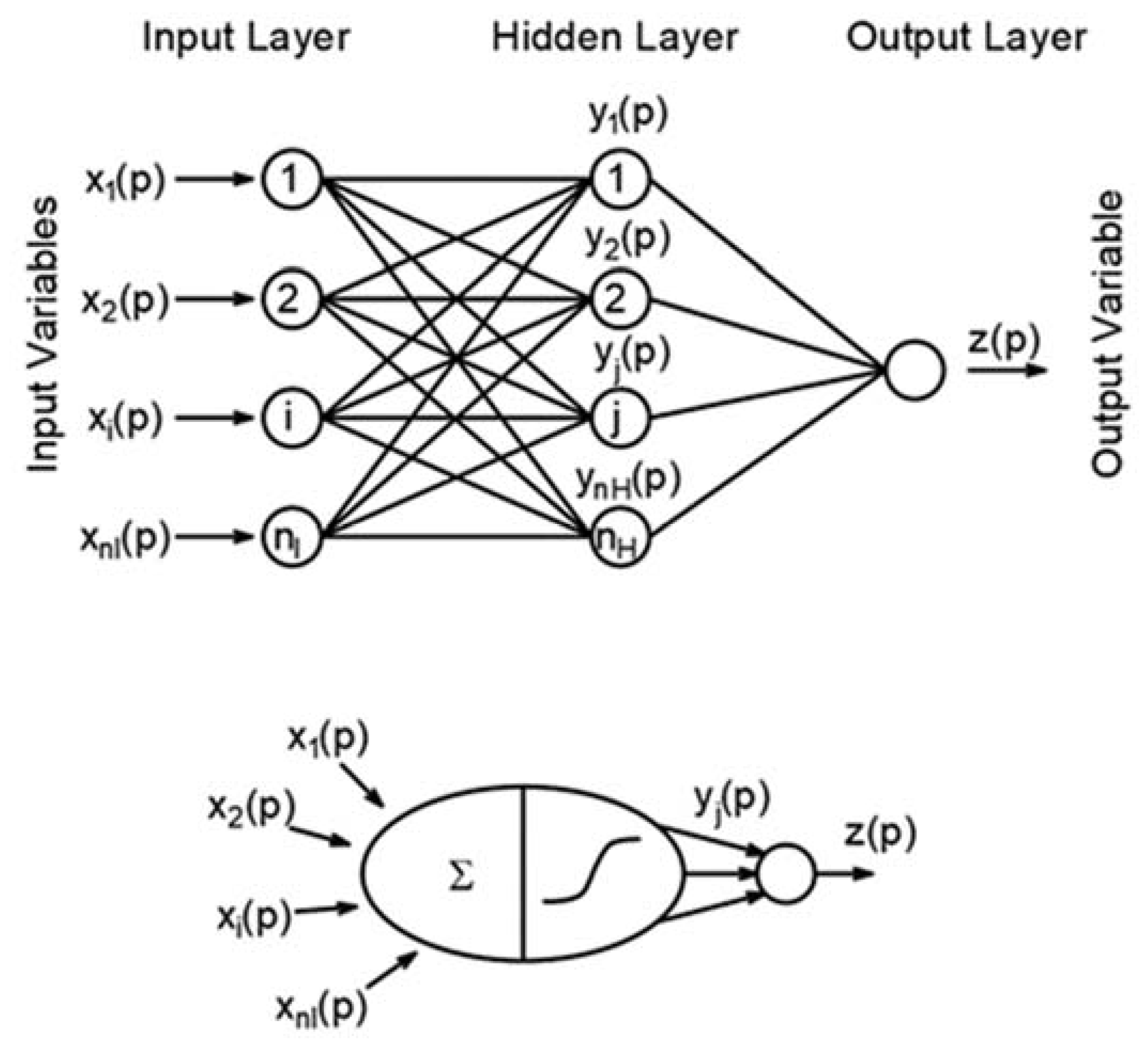
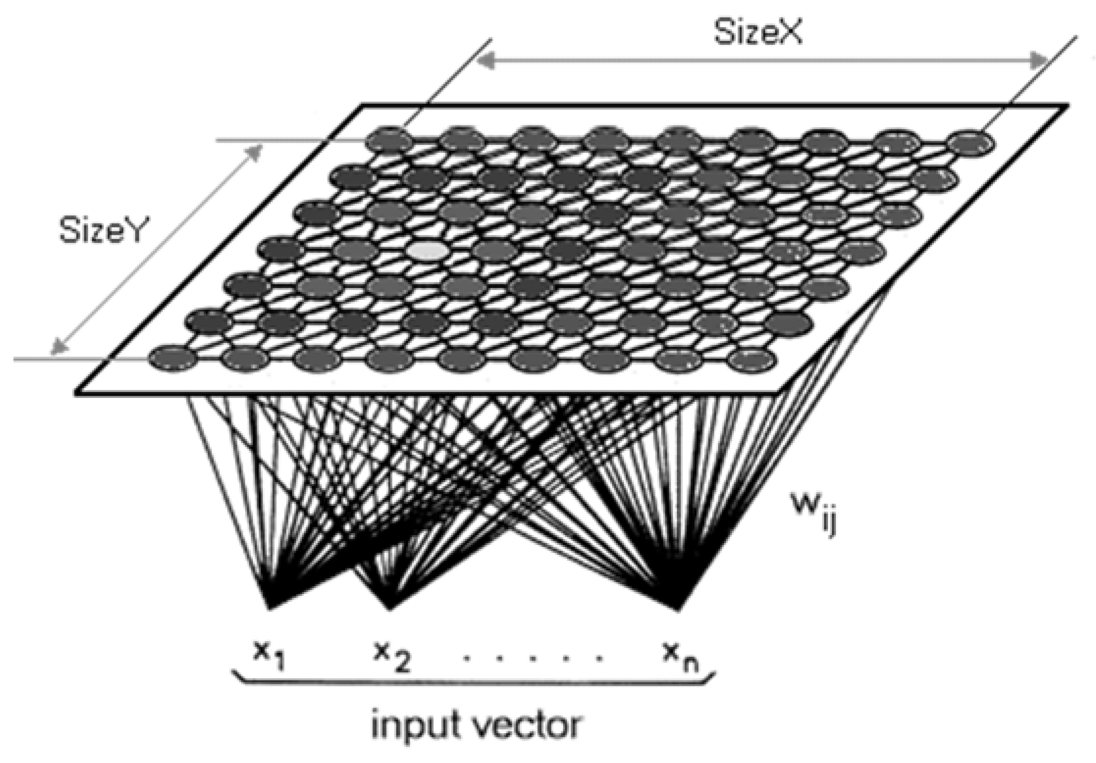
2.3. Artificial Neural Network in the Application of Energy Consumption Diagnostics and Kohonen Maps

When evaluating hourly electricity consumption, individual load diagrams are gradually evaluated over the course of one year. Obtaining the resulting consumption type diagram for a given day of the week and year is a complex issue. The type daily diagram can be obtained by applying neural networks and cluster analysis. The type daily diagram is then the optimized electricity consumption in the area. The control system defines and controls the required electricity production in hours.
Therefore, the definition of an artificial neural network (ANN) will now be discussed for its algorithm to be used for the presented solution [32,33].
ANN is defined as an oriented graph. This graph G is defined as a pair (V, E), where E is a subset of the Cartesian product V × V. Elements E are called arrows or oriented edges. The oriented edge e has the shape (x, y). We say that this oriented edge starts from x and ends in y. It is an ordered group of five [V, E, ε, w, y], where:
  • V V-a set of points (neurons), or a population of neurons
  • E —a group of network edges, called synapses
  • ε —display of edge–vertex incidence ( ε : E V × V )
  • w —dynamic edge evaluation ( w : ε ( E ) × T )
  • y —dynamic vertex rating ( y : V × t )
For T T and t t , w ( [ i , j , T ] ) w i j ( T ) and y ( [ i , t ] ) y i ( t ) is a scalar, resp. y ( t ) = [ y 1 ( t ) | i V ] is a vector which in our case means a certain state of the neural network at a given time t . Likewise, w ( T ) = [ w i j ( T ) | [ i ,   j ] V × V ] is also a vector quantity with a certain neural network combination and is a function of time T . We further define [ i ,   j ] ε ( E ) w i j ( T ) = 0 . Now we can assume that this combination or state of the neural network is a vector quantity that is a function of time T or t . This process is called adaptive dynamics (active dynamics) ANN.
By distinguishing the times of adaptive and active dynamics, it was understood that the ANN works in two time-independent modes. These modes define adaptive and active dynamics. Adaptive mode is a network learning process. This means setting the neural network configuration so that they result in so-called patterns presented by the neural network and their corresponding associations: The active mode works by implementing a network function, the so-called learned function. In the adaptive mode, the state of the network is taken as a consequence, and a stimulus is applied to the neural network.
We again define the active and adaptive dynamics of ANN as a vector quantity on the platform for solving a system of differential equations:
d d t x j ( t ) + x j ( t ) = i f i ( x i ( t Δ t ) ) w i j ϑ j
d d T w i j ( T ) + β g j ( x j ( T ) ) w i j ( T ) = α f i ( x i ( T ) ) g j ( x j ( T ) )
where for i , j V , α , β 0 , 1 and Δ t > 0 expressing the signal delay, then:
Note: x i is the output of the i-th neuron, f i is the transfer (activation) function of the i-th neuron ( f i ( x i ) = y i ) , g j is the output of the i-th neuron, ϑ j is the threshold of the j-th neuron, w i j are the weights (bonds) neuron (i-th with j-th neuron). is the degree of synapse plasticity, β is the degree of synapse elasticity and Δ t is the signal time delay.
In another mathematical survey, see [33], we arrive at an introduction to the adaptive regime and the training set.
The state dependency on the neuron potential (activation function) is approximated by a sigmoid:
f ( x ) =   1 1 + e p x   where the parameter p > 0   represents the steepness of the sinusoid and x is the internal potential of the neuron.
The first enhancement of the perceptron is the various activation functions. For steepness approaching zero or infinity, the activation function is then obtained in the form of linearity (adaptive mode) and finally, hard nonlinearity (training set), see [33].
The following step gives an equivalent formulation of the neuron’s internal potential and the neuron’s activation function [33].
x j = i y i w i j   f ( x ) = 1 1 + e p ( x ϑ )
The parameter ϑ is understood as a neuron threshold, non-achievement or exceeding of which by the neuron potential inhibits or excites the neuron, respectively. The above-mentioned leads to the following conclusions:
  • The neuron excitation is between 0 and 1 , where the value of 1 means full excitation of the neuron as opposed to a value of “0”, which corresponds to a state of inhibition (damping),
  • If the internal potential of the neuron approaches the value + , the so-called complete excitation of the neuron will occur, then this will mean y = f ( + ) = 1 ,
  • Conversely, if the internal potential approaches the value of , then full inhibition of the neuron occurs, i.e., y = f ( ) = 0 .
In the original formulation of the neuron’s potential and activation function, there is:
    x j = i y i w i j ϑ j   f ( x ) = 1 1 + e p x
The parameter ϑ can be understood as an external stimulus that activates the network by injection directly into the neuron, at which value the neuron’s potential is initiated: x j ( 0 ) = ϑ j , then the vector x ( 0 ) = [ x j ( 0 ) | j V ] is the network’s input; the network’s output is understood as the network state.
A vector function, assigning the network input at time t to the network output at time t + Δ t , is called a network function:
F ( x ( t ) ) = y ( t + Δ t )
where Δ t is the network activation (response) time, wherein the network configuration is a parameter of the network functions.
The set of network inputs injected into the network during adaptive dynamics is called the training set:
{ x ( T ) | T Δ T }
where Δ T is the network adaptation (learning) time.
To teach the ANN, we have a training kit that includes elements describing the problem. Furthermore, a method that can fix neural network patterns in the form of synaptic weights, including the possibility of their generalization. Each pattern of the training set describes how the input and output layer neurons are excited. Formally, the training set T can be defined as a set of elements (patterns) that are defined as ordered pairs:
T = { { I 1 ,   O 1 }   { I 2 ,   O 2 }       { I p ,   O p } } ,   I i = [ i 1   i 2     i k ] ,     i j 0 ,   1 ,   O i = [ o 1   o 2     o m ] ,   o j 0 ,   1
In relation (33), the parameter is p , which expresses the number of training set patterns. The parameter I i expresses the so-called excitation vector of the input layer, which represents k neurons. O i is then the excitation vector of the output layer, which is formed by I neurons and finally i j ,   o j is the so-called excitation of the j-th neuron of the input or output layer.
The analysis was performed, and the artificial neural network was mathematically defined. The neural network learning process was described; it is necessary to solve the presented issue (experiment). Now, in terms of UC solutions, the focus will be on the neural network by describing competition, Kohonen learning and self-organization.

2.3.1. Competitive Network Model

ANN consists of neurons, mathematically described, simple elements that process input information (signals) and vice versa generate output signals (information). ANN has a topological arrangement of individual neurons, which are structurally grouped, and communicate according to oriented edges, so-called value connections.
The basic idea of the ANN concept is demonstrated on the principle of the most used forward multilayer neural network. Such a neural network consists of several layers of perceptrons, see Figure 8 [34], which is modified for the sake of our experiment. The perceptrons of individual adjacent layers are interconnected to form a complete biparity graph. The output of one layer neuron is distributed to the inputs of all perceptrons of the next layer. That is, each perceptron of the next layer has as its inputs the outputs of perceptrons from the previous layer. Perceptron inputs from the previous layer are also distributed. The last layer of perceptrons is called the output layer, the other layers of neurons are called hidden layers. Similarly, the perceptrons of these layers are called output or hidden.
The process of equipment and learning in the multilayer ANN, which takes a stand in this research (experiment) needs to be understood we, therefore, refer to [33], where this issue is described in detail.

2.3.2. Kohonen Network

The Kohonen Self-Organization Map (SOM), or Kohonen Network, is one of the networks that function as teacherless learning [35].
The data is plotted to show the relationships between them, in a low, typically two-dimensional array. This will determine if the unmarked data has any structure, see Figure 9.
The triggering process in the Kohonen network is based on the fact that in the first place the distances d j between the presented pattern and the weights of all neurons are calculated, according to the relation
d j = i = 1 m ( x i w i j ) 2 ,
where the index j is part of all neurons in the competence layer, m is the number of neurons, x i are the elements of the presented pattern and w i j indicates the weights of the neurons. Subsequently, the neuron j * whose distance is minimal from the presented pattern is selected, i.
d j * = min j ( d j ) .
Note, that the output of said neuron is active, but the outputs of other neurons are inactive.
If it is an application of cluster analysis, then it does not use a dependent variable (i.e., learning without a teacher), but its goal is to detect non-trivial clusters in the data. In this case, it is the Kohonen network.
During learning, we gradually present training patterns in random order. In our case, when searching for a type of daily diagram, these are the load diagrams of individual consumers in a given urban area, in our experiment. Subsequently, for each of these patterns (load diagram), we find the corresponding nearest neuron, as in the case of triggering. The individual weights of the winning neuron or neurons in its vicinity are adapted by the relation:
w i j ( t + 1 ) = w i j ( t ) + η ( t ) h ( υ ,   t ) ( x i ( t ) w i j ( t ) ) .
Learning parameter η ,   0 < η < 1 , determines the size of changes during the adaptation of the scales. This parameter is set to a value that is close to one. During learning, this parameter decreases to zero. Subsequently, around each neuron, its surroundings are defined, in which weight changes will be made, but only if this neuron is selected in the competence.
In relation (36), is i = 1 ,   2 ,   ,   n   u n d   j = 1 ,   2 ,   ,   n . The neighborhood function h ( υ ,   t ) defines the extent of cooperation between neurons, i.e., how many weight vectors adjacent to the winner will also be adapted and to what extent. The easiest feature to use is the rectangular neighborhood
h ( υ ,   t ) = 1 ,   i f   D M ( υ ,   t ) η ( t ) ;   0 ,   otherwise
where D M ( υ ,   t ) , represents the Manhattan distance D B ( x i ,   x j ) = l = 1 m | x i l x j l | = | x i x j | , between υ   u n d   t neurons in the map grid (sum of absolute values of differences in their coordinates). If the objects xi and xj are characterized by two variables, we can represent their distance in two-dimensional space according to [35].
The best results can be achieved when the size of the neuron’s environment decreases with time (Kohonen). The diameter of the surroundings corresponds to the value 2 η ( t ) .

3. Results

3.1. Experiment, Interpretation of Problems and Results

3.1.1. Experiment Description and Assignment

In solving the concept of sustainable energy in terms of local application of renewable energy sources (RES) in public space, we focused on applying this issue at the level of research. For this purpose, we have selected the territory of the Prague 6 district, see Figure 3.
There are several ways to address energy savings in buildings. This investigation seeks to propose an optimization that will affect the balance between electricity production and consumption in a given urban area. This project is examining this issue in an experiment. This research was, therefore, focused on the solution of the Unit Commitment application in the local urban area consisting of six blocks of buildings marked with the letters A, B, C, D, E and F. Photovoltaic power plants under the designation PV1, PV2, PV3, PV4, PV5 and PV6 on units A, B, C, D, E and F. This project local micro-network of RES meets the condition for the construction of buildings with almost zero energy consumption-NZEB (Neatly Zero Energy Buildings), Table 1. Their structure within the urban area was adjusted to address the Unit Commitment (UC) of the presented experiment. This research was the main goal of addressing the energy performance of buildings, including reducing CO2 emissions.
The local microgrid of distributed RES systems (photovoltaic systems (PV)), energy from biomass, cogeneration, battery storage and energy distribution (22/0.4 kV) is shown in Figure 10, is part of the Smart Micro-Grid (SMG) control within the UC system.
The local RES network is concentrated in the city’s energy center (CEC). Individual characteristic values, such as nominal outputs of individual PV systems, distribution system outputs including cogeneration and technical limitations of individual sources, are given in Table 2. Table 3 shows the annual values of PV energy production in the context of the number of panels for individual building blocks A, B, C, D, E and F.
Note in Table 2: We start from relation (14), where Pn is the nominal output of PV plants based on RES, including the fact that we adjust the total consumption with the present time of 0.7.
This investigation also focused on a more comprehensive view of energy savings within the urban area, as it also has a significant effect on the CO2 reduction platform. Therefore, this research also focused on the estimation of electricity consumption in the named part of the city (experiment). This estimate is based on the total usable floor area of all buildings (blocks of type A, B, C, D, E and F). For this purpose, the buildings were divided into typical brick blocks and blocks of flats. From this research, the total electricity consumption per year was evaluated, and shown in Table 4.
Table 4 evaluates the values of electricity consumption, heating energy and hot water preparation depending on the current state of building construction (type blocks) and the new state of buildings (type blocks), i.e., before and after the reconstruction of buildings. Table 4 shows the energy savings, where due to the reconstruction of buildings, we will achieve the greatest savings at the level of heating. For example, for Type block: No. 1004, we achieve up to 45% energy savings for heating and 7.2% energy savings, and with block no. 1020 to 75% energy savings for heating and 5.9% electricity savings.
Due to the fact that the structures do not meet the requirements of NZEB, the following changes were made: putting the heat transfer coefficient of the building envelope to the standard values (insulation of walls, structures in contact with the ground, roofs). The simulation was performed using DesignBuilder software for later comparison of energy savings. The results are shown in Table 4 and Table 5, for the type of block and apartment buildings. This means that the current state is not satisfactory in terms of heat transmission through building structures and after the reconstruction of the simulations, we achieve satisfactory values in comparison with the required standard values.
The conclusions and their presentation in Table 4 and Table 5 show that this research needs to be extended and subsequent solutions to energy intensity in the position of reducing electricity consumption are needed. The reduction in electricity consumption is visible but can be further influenced. The reduction of energy in the heating position is sufficient and transparent with the requirements of Decree No. 264/2020 Coll. on the energy performance of buildings published on 5 June 2020 in the phase of its legislative approval. Decree No. 264/2020 Coll. takes effect on 1 September 2020 and replaces the current Decree No. 78/2013 Coll. Thus, this research focused only on reducing electricity consumption, which will be described in Chapter 3.1.2 Type Daily Diagrams of Energy Consumption, Application of the Cluster Analysis Method, and Kohonen Map.

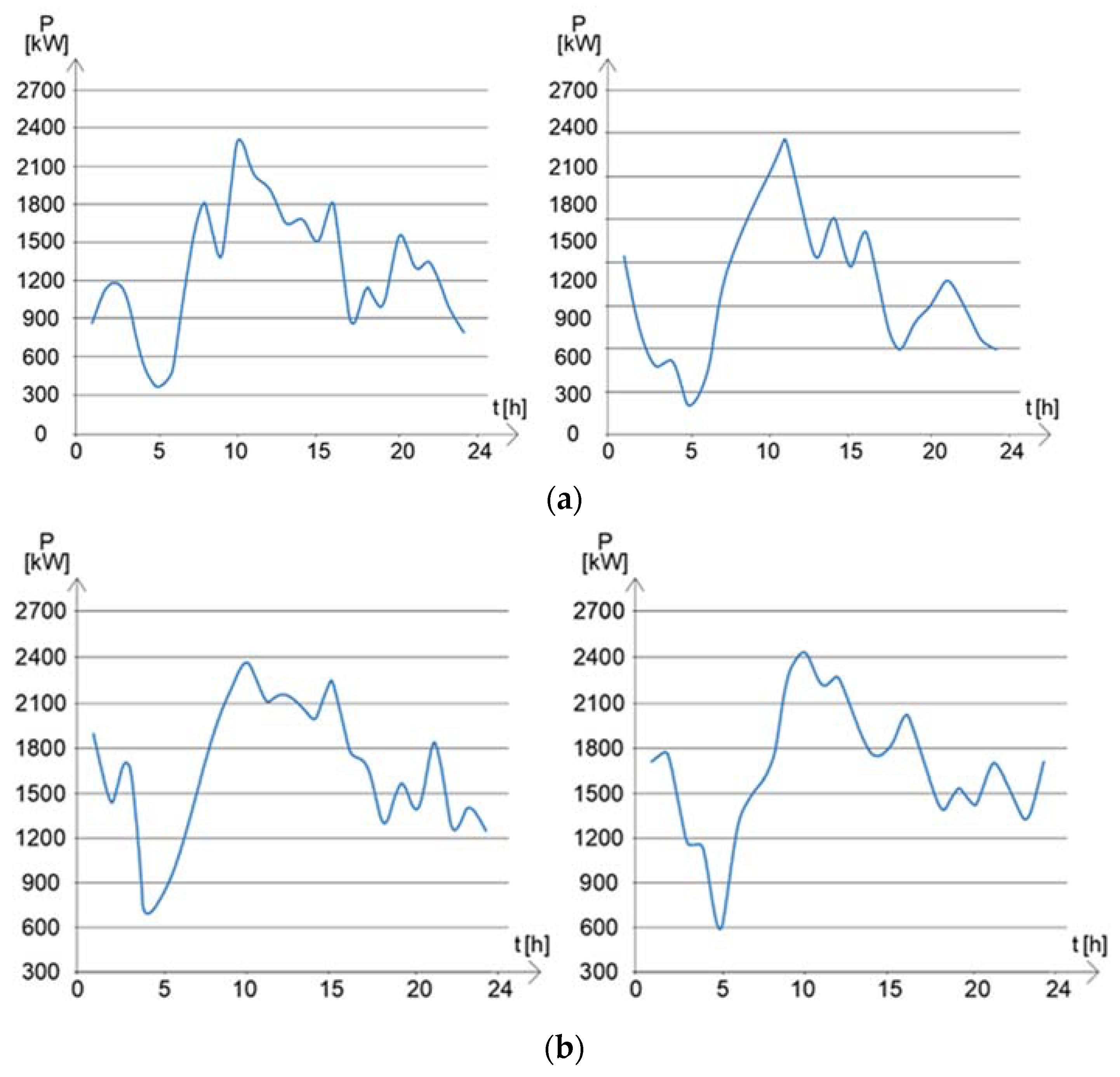
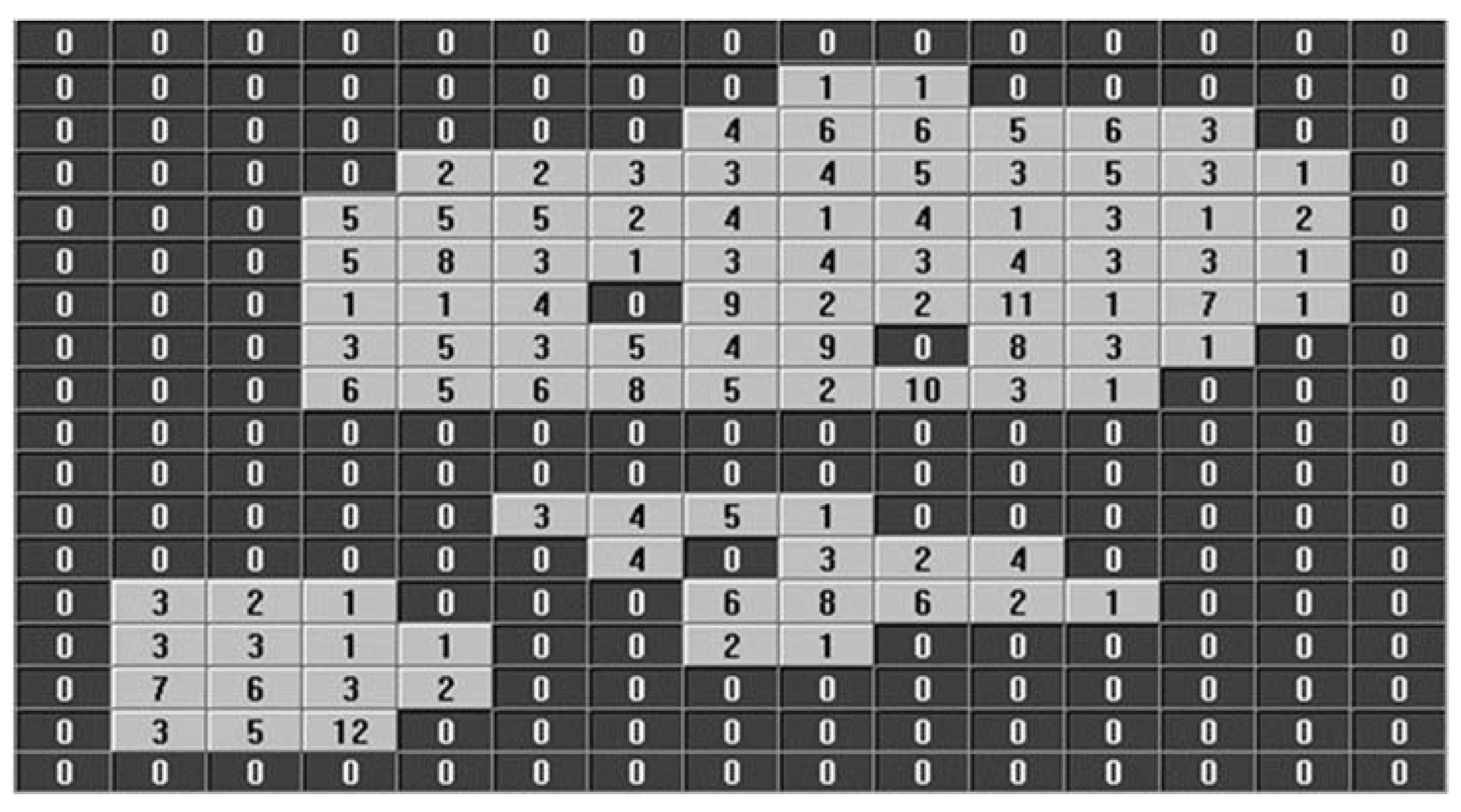
3.1.2. Experiment TDD Energy Consumption, Kohonen Map Application

Today, the development of electricity production from RES is an effort to maximize the share of total energy consumption. The RES microgrid is connected to the distribution network in case the supply of electricity from the solar power plant (PV1, PV2, PV3, PV4, PV5, PV6) including electricity from the battery storage is not available. Our project is designed as an energy source, which is a combination of solar micro RES and batteries so that electricity is supplied throughout the day. The article deals with the study of electricity consumption of apartment buildings (blocks A, B, C, D, E and F), both residential and commercial.
The building and construction sectors worldwide are showing an increase in emissions and energy consumption. It is, therefore, necessary to provide certain measures to reduce emissions and achieve a low-carbon sustainable built environment. The current built environment needs to be revised in order to achieve a different way of reducing energy consumption and thus CO2 emissions. In our case, the means to do this is supported by research into sustainable energy in the context of energy savings on the part of consumers. A very effective tool for this is the application of artificial intelligence, especially the use of neural networks, cluster analysis, optimization methods and unit commitment in electricity supply management. In addition, it is necessary to ensure the reconstruction of buildings to meet the requirements of NZEB. Subsequently, we can proceed to the proposed solution, which in our case is UC.
To solve the UC RES microgrid in our research, it is necessary to address the issue of electricity consumption identification, i.e., find type daily charts (TDC) in a given urban area. In addition to estimating consumption of the point of consumption, they are also an integral part of the systems for electricity trading and for systems of settlement of electricity deviations, where they replace the determination of the amount of hourly consumption of a group of customers. To determine the course of consumption from the recalculated type diagrams of deliveries, a formula is used to calculate the amount of consumption in a given hour:
O h = O r · r h h = 1 8760 r h
where O h is the amount of consumption in a given hour, O r is the total annual consumption of the offtake point and r h is the size of the relative value of the normalized TDC of the relevant category and h is the number of hours.
In our experiment, the goal is to define and identify TDC hourly electricity consumption. For clarity and a simplified presentation of the results, we chose two days a week, which are Thursday and Saturday. The individual TDCs were created on the basis of the annual consumption history. For this purpose, we will use cluster analysis, where the relevant annual history of hourly consumption was artificially modeled. Subsequently, these TDCs were compared with a standard that was identified by (38). Furthermore, the knowledge of Decree No. 541/2005 Coll., on the rules of the electricity market in the Czech Republic, was used. There are estimates of the likely course of consumption of a particular consumption point over time, taking into account a number of factors that affect consumption modelling [20].
From the results of TDC modeling of the annual history of electricity consumption in the area, we found that the resulting daily diagrams differ significantly, see Figure 11 (Thursdays) and Figure 12 (Saturdays). Nevertheless, TDCs are very similar to the relevant standards, see Figure 12 and Figure 13. This fact confirms the high efficiency of the cluster analysis method. This method ensures the maximum possible approximation and thus the conformity of TDC with their copies and standards. Then the UC RES application in the power and production management system has a minimum deviation. This will achieve significant savings in electricity in the area. As already mentioned, this calculation and TDC survey was carried out in September 2021. The individual hourly consumptions were modeled using a random number generator. It has been modeled 69 times using the PYTHON program. Figure 13 shows two examples of randomly modeled diagrams of daily working days on Thursdays.
If we look at the course of electricity consumption, then we can see in Figure 11 and Figure 14, which show the daily diagrams of electricity consumption at the time level of one year, that they differ greatly from each other. It follows that TDCs are quite similar to the relevant standards.
Basically, it is a matter of sorting units into groups (clusters) so that units belonging to the same group are more similar than objects from different groups.
The above-mentioned individual daily diagrams of the annual history, see Figure 11 and Figure 14, differ considerably from each other, so the typical daily diagrams are quite similar to the relevant standards, see Figure 13 and Figure 14,
In our case, when observing the above Figure 11, Figure 12, Figure 13 and Figure 14, it can be stated that the cluster analysis method is very effective.
In addition, Table 6 contains a numerical comparison of the type of daily diagrams with the relevant standards. Here we can see that their average and maximum deviation (difference) are in the range of about 0.08% and 0.52% respectively. From these results, it can also be concluded that the cluster analysis method appears to be a very efficient and high quality accurate method, as shown in the presented experiment. The experiment was processed in the computer program PYTHON.
Kohonen map
Our experiment is based on the resulting TDC, according to which the production and consumption of electricity in the UC system, i.e., the RES microgrid in the given urban area, will be controlled and optimized. For this purpose, we consider the application of the Kohonen network. We consider a set of training patterns that have been randomly and evenly selected. The task was then to represent their division. In any case, the resulting distribution of neurons in space should correspond to the nature of the probability distribution of training patterns. Such a model is in its form analogous to cluster analysis. During adaptive dynamics, the training set forms multidimensional data that is grouped into a 15 × 15 square matrix. The network topology contains two layers of neurons with 364 rows and 24 columns. We verified that the degree of plasticity decreased exponentially from the initial value of 1 to a final value of 0.005 during network adaptation. We also found the order of the gain neuron, which decreased exponentially from the initial value of 7 to the final value of 0, i.e., the neighborhood of the gain of the basic order gain neuron covered the entire grid of the output grid layer. The result of the experiment is a Kohonen map Figure 15. From this map you can read three well-separable clusters, the highest point of the map and two less pronounced clusters probably corresponding to Saturday or Sunday and one clearly visible cluster probably representing the working day Thursday.
At the end of the Kohonen map application, TDCs can be found, which are shown and compared with the relevant standard, see Figure 16. This result is relevant and demonstrates the most optimal solution in the UC process of the RES microgrid in the given area of our experiment.

3.1.3. Experiment Proposal for Unit Commitment of the RES Micro-Network in the Given Area

The system Unit Commitment (UC) of the RES microgrid is located in the city’s energy center (CEC). This UC project is supported by KNX technology, which is an open standard called EN 50090 or ISO/IEC 14543 and is used for the automation of commercial or domestic buildings, but also for energy management. Its goal is the optimal management of electricity supply to the defined area. This research concerns the city district of Prague 6 (see experiment). The process of electricity supply management in a given area implements the allocation of individual energy sources over time according to Table 7. Where the values of UC variant 2, which were accepted, are expressed. Other variants are only evaluated in the text of Table 8.
The calculation time on a laptop equipped with a 2 GHz processor was two minutes and thirty seconds.
In this experiment, the complex is powered by ten synchronous generators (including battery storage), whose cost characteristics and technical limitations are listed in Table 2.
The experiment aims to design the order of resources for a typical working day (Thursday), for which predictions of hourly consumption are available, see (Figure 16).
The starting point of the solution is the process of setting the parameters of the optimization algorithm T0 resp. T∞ resp. N, which were set to values of 100 resp. 10-6 resp. 105 per experiment. Now the process of setting the initial temperature is based on the initial estimate and subsequent increase to the value where during the first about ten percent of iterations are accepted almost all faults, which is similar to heating the object during annealing (optimization algorithm simulated annealing). Similarly, this mechanism for setting the final temperature was based on its initial estimate and subsequent reduction of the temperature to a value where during the last about ten percent of iterations almost no faults increasing the value of the cost function are accepted.
The assumption of the mechanism for setting the number of iterations was based on estimation and subsequent gradual increase up to the value so that its further increase would not lead to a significant reduction in final production costs for the required amount of energy.
The calculation of the value of the purpose function (20) is given in the source code section of the computer program in PYTHON (Algorithm 3).
The algorithm proposes power allocation for each hour within a defined period and for each iteration, see Table 7.
Algorithm 3. Part of the source code of the purpose function value calculation (20)
for (j = 2; j <= nt + 1; j++):
for j in range (2, nt + 2): # iterace 2 až nt + 1
  for iter in range(1, n+1):
    i = random(seed) * (ng − 1) + 1
    ij = (i − 1)*(nt + 1) + j
    if x(ij) == 0:
      if random(seed) < Ponoff:
        x(ij) = 1
    else:
      if random(seed) < Ponoff:
        x(ij) = 0
    i = random(seed) * (ng − 1) + 1
    ij = (i − 1) * (nt + 1) + j
    p(ij) = random(seed) * (Pmax(i) − Pmin(i)) + Pmin(i)
Where nt is the number of hours and ng is the number of available resources, p(ij) is the power of the i-th source and the j-th hour, x(ij) is the state of the i-th source and the j-th hour. Pmin and Pmax are the power limits of the i-th source. Ponoff is a parameterizable probability of the source state change, and the random function is the said random number generator from the interval (0, 1) with even distribution of probability. The result of our experiment from the source organization position for said Wednesday is shown in Table 6. Finally, a remarkable fact is that time of calculation made by a laptop was two minutes and 30 s.

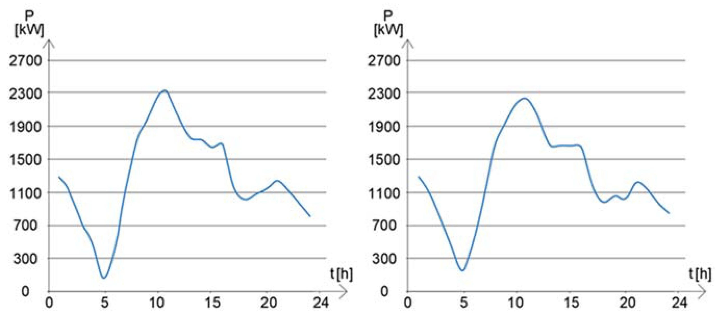
3.1.4. Analysis of Experimental Process Results

Although there are countless published articles on UC, this research has focused on the issue of next-generation UC in regulated, deregulated, and sustainable energy. The proposed two-stage process uses AI, through a neural network to generate a preliminary UC plan according to the input load profile. Experimental results suggest that the proposed algorithm can significantly reduce the execution time of the traditional dynamic programming approach without compromising the quality of the generation plan.
Efficient and optimal operation and planning of electricity generation systems have always played an important role in the power industry. The problem of economic operation in electricity systems also includes the planning of both thermal units (biomass), battery electricity, central electricity and cogeneration units in order to minimize energy supply costs.
The optimal operation of cogeneration units involves minimizing fuel consumption. Estimates have shown that a 1% reduction in production costs can result.
This research deals only with the planning of electricity generation, which can be considered a major part of the problem of energy system planning. Unit Commitment is the problem of selecting generating units to be in operation during the planning period and for how long. Certified units must meet system load requirements and reserves at minimum operating costs, subject to various restrictions.
The economic problem of dispatch control is the optimal distribution of load demand between running units while meeting the energy balance equations and operating limits of the units (20).
The UC solution is a complex optimization problem. The solution is based on two interconnected optimization problems. The first is a combinatorial problem and the second is a nonlinear programming problem.
The exact UC solution can be obtained by a complete enumeration of all possible combinations of generator units, of which there can be a huge number. The solution methods used to solve UC can be divided into four categories [36,37,38,39,40,41,42,43,44,45,46,47,48,49,50,51,52,53,54,55,56]:
  • Classical optimization methods, such as Dynamic programming, Lagrange relaxation, Linear programming, Integer and Mixed Integer Programming, Probabilistic Methods, and Network Flow Programming [57,58,59,60,61,62,63,64].
  • Heuristic methods and expert systems [65,66,67,68,69,70,71].
  • Artificial intelligence methods, e.g., Simulated annealing, Neural networks, Taboo Search and Genetic algorithms [72,73,74].
This research presents the application of a simulated annealing algorithm (SA) to solve a UC problem. New rules for random generation of feasible solutions are introduced here.
The importance of the UC system grows with ever-changing requirements. Therefore, in the energy sector, within the framework of energy sustainability, there is an urgent need to follow the latest methodologies for further optimization of the working criteria of production units or energy units (RES). The experiment, therefore, focuses on describing an overview of the latest techniques in the field of artificial intelligence used in optimizing UC problems for stochastic and deterministic loads. The various sections of the UC solution include various restrictions based on profit, safety, emissions (CO2) and time.
The main emphasis is on deregulated and regulated environments, especially renewable energy sources and distributed generation systems.

4. Discussion

In the given area of the building cluster, the necessary parameters and requisites for assessing the current state of the EPB were identified through measurements, inspection, and the use of building documentation. The structures were found not to meet the requirements for will NZEB; therefore, the following changes were made: bringing the heat transfer coefficient of the building envelope to standard values (insulation of walls, structures in contact with the ground, roofs). The results and comparison with the original state are shown in Table 3 and Table 4. Table 3 evaluates the results of savings in each key commodity that have occurred due to the application of EMB (Note: Only two blocks were evaluated, namely: Type block No. 1004 and Block of flats No. 1020. There are a total of 28 blocks of flats and three type blocks in the given area. The building design, structure, and heat transfer coefficients are identical for each block, so the tabulated values in Table 3 are taken as unit values. The total value of consumption, water, heat, and electric power could be multiplied by the number of blocks, which is 31 blocks, to achieve 90 to 95% accuracy of individual commodities).
(a)
Heating: In this case, the energy consumption due to building renovation in the given area decreased by 54.9%, i.e., almost twice for the type of block and by 75.50%, i.e., almost four times for the block of flats.
(b)
Hot water preparation: In this case, the energy consumption in the type of block increased by 3.7% even though the buildings in the given area were renovated. So, the energy consumption for hot water preparation was not affected. As for the energy consumption for hot water preparation in blocks of flats of the given area, there was a 6.66% reduction in energy consumption.
(c)
As for the reduction in electric power consumption due to building renovations in the given area, the results are as follows:
  • Electric power consumption decreased by 7.27% in the type blocks.
  • Electric power consumption decreased by 5.96% in the blocks of flats.
These partial conclusions suggest that further focus is needed on electric power consumption and addressing energy sustainability. The installation of a RES microgrid, see Figure 10, together with system control and optimization of the stable energy balance, is believed to be an essential feature of this solution.
At this point, it should be emphasized that the operator of the RES microgrid within the local distributed transmission system balances the instantaneous power deviations in MW or business units in MWh. The main reason for this is the 1-h settlement trading interval, and the deviation means the difference between the actual and agreed supplies or withdrawals for the previous trading interval. Thus, this so-called local dispatching system of a given urban area is ready to implement community power engineering.
The implementation of the UC platform in the context of energy balance management is a process of applying artificial intelligence (AI) in addressing sustainable power engineering, reducing energy consumption and CO2 production, including promoting environmental quality. This process is based on applying neural networks, cluster analysis, and evolutionary computing.
Last but not least, the application of an automated management system for technical building installations (TBI) impacts the energy consumption of the houses in a given urban area.
The application of artificial intelligence is a very important step towards strengthening the energy performance of buildings and, in this context, reducing energy consumption and CO2 emissions. In this context, we applied cluster analysis and Kohonen’s map. Interesting results of such a solution are shown in Table 6. It can be observed that interesting indicators are evident at the level of average and maximum tolerance between the type daily diagram (TDC) and its standard range. They range between about 0.1% and 0.52%.
It represents significant effects in the process of reducing electric power consumption. For example, if the tolerance between the TDC and its standard is 0.1%, the consumption of 1 MWh/year in the given urban area results in savings of up to 1000 kWh/year. It confirms the great importance of AI applications in the energy management process. Each tenth of a percent of tolerance represents 1000 kWh/year. Without using the cluster analysis and Kohonen map, the tolerances of TDC and its standard range from 0.7 to 0.9. With an average tolerance of around 0.8%, using tolerance adjustment through cluster analysis can achieve savings of up to 5000 kWh/year in the given area, representing a saving of 0.5% for a total electric power consumption of 1 MWh/year.
Table 8 gives an overview of the performance balance results for the three solution variants, which were described in the relations: 0 (zero variant) relation (17), 1 (first variant) relation (20) and 2 (second variant) relation (21). Table 7 shows in detail the second variant, which is documented by the calculation values in Table 6. The other variants (zero and first) and their associated results are not documented in the tables. The reason is the large scope of this article. We present only the overall results, which will allow the selection of a variant for the solution of our experiment, Table 8.
From the comparison of the results of the power balance given in Table 8, where only the results of the smallest deviations from the zero power balance are given, the second option was achieved (Table 6).
The second option is based on the use of a fuzzy deviation model (21). Tables with commitment data of the RES microgrid unit for variant “0” and variant “1” are not displayed (so as not to extend the scope of this document); are generally similar to Table 6, but with different values. These values are listed in Table 8, which are sufficient to discuss the problem. The final UC proposal for Option 2 is shown in Table 6. The tables for Options 0 and 1, including Table 6, show Option 2 (reflecting the three deployment source plans for the day, with Option 0 being the constraint (17), that any random solution proposal where the sum of the supplies does not exceed the expected load is automatically rejected and used in variants 1 and 2 by the objective function of forms (20) and (21).
On the contrary, the highest deviations from the zero power balance were achieved in variant 1, see Table 8. The reference costs, including the costs of electricity consumption in the period under consideration, were the costs of permanently operating energy sources, i.e., CZK. 4730 being the most common, Table 8 shows the maximum deviations from the zero power balance in kW and the size of the deviation from local electricity suppliers (in the Czech Republic it is ČEZ) in kW, including the total energy costs of sources integrated into the microgrid in CZK (Czech crowns) for the whole planning day.
From the point of view of the requirement of energy self-sufficiency of a complex of intelligent buildings, fuzzy formulations restrictive conditions seem to be the best way to accept it (17). It is not desirable to compensate the balance for the costs of the regional electricity distributor in the Czech Republic in either of the two directions.

5. Conclusions

If the results obtained in the experiment are evaluated, then it is possible to evaluate:
  • Used artificial intelligence methods: cluster analysis, neural networks, Kokonem map and simulated annealing (as an optimization algorithm), in the design of UC solutions of local energy sources, such as RES have established themselves as a very effective chronological method of sustainable energy solutions within NZEB.
  • Use in future practice: The fuzzy condition in UC design has been shown to be most effective when a restrictive condition has been adopted (21). UC has significant potential, especially in addressing energy savings and thus reducing emissions, such as CO2.

Funding

This research received no external funding.

Conflicts of Interest

The authors declare no conflict of interest.

References

  1. Streimikiene, D.; Balezentiene, L. Assessment of Electricity Generation Technologies Based on GHG Emission Reduction Potential and Costs. Transform. Bus. Econ. 2012, 11, 333–344. [Google Scholar]
  2. Streimikiene, D.; Mikalauskiene, A. Barakauskaite-Jakubauskiene. Sustainability Assessment of Policy Scenarios. Transform. Bus. Econ. 2011, 10, 165–168. [Google Scholar]
  3. Streimikienė, D.; Mikalauskienė, A.; Mikalauskas, I. Comparative Assessment of Sustainable Energy Development in the Czech Republic, Lithuania and Slovakia. J. Compet. 2016, 8, 31–41, ISSN 1804-171X (Print), ISSN 1804-1728 (On-line). [Google Scholar] [CrossRef]
  4. Cicea, C.; Marinescu, C.; Popa, I.; Dobrin, C. Environmental efficiency of investments in renewable energy: Comparative analysis at macroeconomic level. Renew. Sustain. Energy Rev. 2014, 30, 555–564. [Google Scholar] [CrossRef]
  5. Ibáñez-Forés, V.; Bovea, M.D.; Pérez-Belis, V. A holistic review of applied methodologies for assessing and selecting the optimal technological alternative from a sustainability perspective. J. Clean. Prod. 2014, 70, 259–281. [Google Scholar] [CrossRef]
  6. Vasauskaite, J.; Streimikiene, D. Review of Energy Efficiency Policies in Lithuania. Transform. Bus. Econ. 2014, 13, 628–643. [Google Scholar]
  7. Streimikiene, D.; Sarvutyte, M. Impact of renewables on employment in Lithuania. Transform. Bus. Econ. 2013, 11, 167–184. [Google Scholar]
  8. Banos, R.; Manzano-Agugliaro, F.; Montoya, F.G.; Gil, C.; Alcayde, A.; Gómez, J. Optimization methods applied to renewable and sustainable energy: A review. Renew. Sustain. Energy Rev. 2011, 15, 1753–1766. [Google Scholar] [CrossRef]
  9. Abujarad, S.Y.; Mustafa, M.W.; Jamian, J.J. Nedávné přístupy jednotkového závazku v přítomnosti občasných obnovitelných zdrojů energie: Přehled (Recent unit commitment approaches in the presence of intermittent renewable energy sources: Overview). Obnovit. Udržet. Energ. Rev. 2017, 70, 215–223. [Google Scholar]
  10. Rasoul, N.M.; Maigha, M.; Jhi-Young, J.; Crow, M.L. Multi-cílový dynamický ekonomický dispečink s řízením domácích zátěží a elektrických vozidel na straně poptávky (Multi-target dynamic economic dispatching with demand-side control of domestic loads and electric vehicles). Energies 2017, 10, 624. [Google Scholar]
  11. Zhanga, X.; Lovatib, M.; Vignab, I.; Widénc, J.; Hana, M.; Gala, C.; Fengd, T. A review of urban energy systems at building cluster level incorporating renewable-energy-source (RES) envelope solutions. Appl. Energy 2018, 230, 1034–1056. [Google Scholar] [CrossRef]
  12. Howell, S.; Rezgui, Y.; Hippolyte, J.-L.; Jayan, B.; Li, H. Towards the next generation of smart grids: Semantic and holonic multiagent management of distributed energy resources. Renew Sustain. Energy Rev. 2017, 77, 193–214. [Google Scholar] [CrossRef]
  13. Garlík, B. Energy Sustainability of a Cluster of Buildings with the Application of Smart Grids and the Decentralization of Renewable Energy Sources. Energies 2022, 15, 1649. [Google Scholar] [CrossRef]
  14. Chang, C.; Kuo, C.C. Network reconfiguration in distribution systems using Simulated annealing. Electr. Power Syst. Res. 1994, 29, 227–238. [Google Scholar] [CrossRef]
  15. GARLÍK, B. The Application of Aetificial Intelligence in the Process of optimizing Energy consuption in intelligent Areas. Neural Netw. World 2017, 27, 415–445. [Google Scholar] [CrossRef] [Green Version]
  16. Minoux, M. Matematické Programování: Teorie a Algoritmy (Mathematical Programming: Theory and Algorithms) (with a Foreword by Egon Balas); Translated by Steven Vajda from the French Edition (1983 Paris: Dunod.); Wiley-Interscience Publications: Chichester, UK, 1986; p. xxviii + 489. ISBN 978-0-471-90170-9. [Google Scholar]
  17. Yang, H.; Yang, P.; Huang, C. Evolutionary Programming Based Economic Dispatch with Non-Smooth Fuel Cost Functions. IEEE Trans. Power Syst. 1996, 11, 112–118. [Google Scholar] [CrossRef]
  18. Wood, A.J.; Wolleberg, B.F. Power Generation, Operation and Control; John Willey & Sons: New York, NY, USA, 1996. [Google Scholar]
  19. Momoh, J. Smart Grid Fundamentals of Design and Analysis; IEEE Press Series on Power Engineering Appears at the End of This Book; Wiley India Pvt. Ltd.: New Delhy, India, 2018. [Google Scholar]
  20. Walters, D.C.; Sheble, G.B. Genetic Algorithm Solution of Economic Dispatch with The Valve-point Loading. IEEE Trans. Power Syst. 1993, 8, 1325–1332. [Google Scholar] [CrossRef]
  21. Lin, W.M.; Cheng, F.S.; Tsay, M.T. An Improved Tabu Search For Economic Dispatch With Multiple Minima. IEEE Trans. Power Syst. 2002, 17, 108–112. [Google Scholar] [CrossRef]
  22. Lee, K.Y.; Sode-Yome, A.; Park, J.H. Adaptive Hopfield Neural Network For Economic Load Dispatch. IEEE Trans. Power Syst. 1998, 13, 519–526. [Google Scholar] [CrossRef] [Green Version]
  23. Eberhart, R.E.; Shi, Y. Comparing Inertia Weights and Factors in Particle Swarm Optimization. In Proceedings of the 2000 Congres on Evolutionary Computation, La Jolla, CA, USA, 16–19 July 2000; Volume I, pp. 84–88. [Google Scholar]
  24. Eberhart, R.E.; Shi, Y. Particle Swarm Optimization: Developments, Applications, and Resources. In Proceedings of the 2001 Congress on Evolutionary Computation, Seoul, Korea, 27–30 May 2001; Volume I, pp. 81–86. [Google Scholar]
  25. Van Laarhoven, P.J.; Aarts, E.H. Simulated annealing. In Simulated Annealing: Theory and Applications; Springer: Heidelberg/Berlin, Germany, 1987; pp. 7–15. [Google Scholar]
  26. Yu, H.; Fang, H.; Yao, P.; Yuan, Y. A combined genetic algorithm/simulated annealing algorithm for large scale system energy integration. Comput. Chem. Eng. 2000, 24, 2023–2035. [Google Scholar] [CrossRef]
  27. Jha, S.; Menon, V. BbmTTP: Beat-based parallel simulated annealing algorithm on GPGPUs for the mirrored traveling tournament problem. In Proceedings of the High-Performance Computing Symposium, Society for Computer Simulation International, Tampa, FL, USA, 13–16 April 2014; p. 3. [Google Scholar]
  28. Kabova, E.A.; Cole, J.C.; Korb, O.; López-Ibáñez, M.; Williams, A.C.; Shankland, K. Improved performance of crystal structure solution from powder diffraction data through parameter tuning of a simulated annealing algorithm. J. Appl. Crystallogr. 2017, 50, 1411–1420. [Google Scholar] [CrossRef]
  29. Assad, A.; Deep, K. A Hybrid Harmony search and Simulated Annealing algorithm for continuous optimization. Inf. Sci. 2018, 450, 246–266. [Google Scholar] [CrossRef]
  30. Zelinka, I.; Oplátková, Z.; Šeda, M.; Ošmera, P.; Včelař, F. Evoluční Výpočetní Techniky (Princip a Aplikace), (Evolutionary Computing (Principle and Application)); BEN-Technická Literature: Praha, Czech, 2009; ISBN 978-80-7300-218-3. [Google Scholar]
  31. Michalewicz, Z.; Fogel, D.B. How to solve it: Modern Heuritics, 2nd, revised and extended ed.; Springer: Berlin/Heidelberg, Germany, 2004. [Google Scholar]
  32. Aarts, E.H.L.; Korst, J.H.M.; Michiels, W. Simulované žíhání (Simulated annealing). In Metodiky Vyhledávání (Search Methodology); Burke, E.K., Kendall, G., Eds.; Springer: New York, NY, USA, 2005; pp. 187–210. [Google Scholar]
  33. Novák, M.; Faber, J.; Kufudaki, O. Neuronové Sítě a Informační Systémy Živych Organism (Neural Networks and Information Systems of Living Organisms); Grada: Prague, Czech Republic, 1993; ISBN 80-58424-95-9. [Google Scholar]
  34. Grim, J.; Hájek, P.; Horaček, P.; Jiřina, M.; Kléma, J.; Kouba, Z.; Mařík, V.; Štěpánková, O.; Laţanský, J.; Kramosil, I.; et al. Umělá Inteligence (Artificial Intelligence) (3); Academia: Prague, Czech Republic, 2001; ISBN 80-200-0472-6. [Google Scholar]
  35. Řezanková, H.; Húsek, D.; Snášel, V. Shluková Analýza (Cluster Analysis); Kamil Msřík-Profesional Publishing: Praha, Czech Republic, 2009; ISBN 978-80-86946-81-8. [Google Scholar]
  36. Catalao, J.P.S.; Mariano, S.J.P.S.; Mendes, V.M.F.; Ferreira, L.A.F.M. Profit based unit commitment with emission limitation: A multi-objective approach. In Proceedings of the IEEE Power Tech, Lausanne, Switzerland, 1–5 July 2007; pp. 1417–1422. [Google Scholar]
  37. Lu, B.; Shahidehpour, M. Unit commitment with flexible generating units. IEEE Trans. Power Syst. 2005, 20, 1022–1034. [Google Scholar] [CrossRef]
  38. Wang, Y.; Xia, Q. A novel security stochastic unit commitment for wind thermal system operation. In Proceedings of the 4th International Conference on Electric Utility Deregulation and Restructuring and Power Technologies (DRPT), Weihai, China, 6–9 July 2011; pp. 386–393. [Google Scholar]
  39. Raglend, I.J.; Kumar, R.; Karthikeyan, S.P.; Palanisamy, K.; Kothari, D.P. Profit based unit commitment problem under deregulated environment. In Proceedings of the 2009 Power Engineering Conference Australasian Universities (AUPEC 2009), Adelaide, Australia, 27–30 September 2009; pp. 1–6. [Google Scholar]
  40. Zendehdel, N.; Karimpour, A.; Oloomi, M. Optimal Unit Commitment using equivalent linear minimum up and down time constraints. In Proceedings of the 2008 IEEE 2nd International Power and Energy Conference (PECon 2008), Johor Bahru, Malaysia, 1–3 December 2008; pp. 1021–1026. [Google Scholar]
  41. Ebrahimi, J.; Hosseinian, S.H.; Gharehpetian, G.B. Unit commitment problem solution using shuffled frog leaping algorithm. IEEE Trans. Power Syst. 2011, 26, 573–581. [Google Scholar] [CrossRef]
  42. Salam, S. Unit commitment solution methods. Proc. World Acad. Sci. Eng. Technol. 2007, 26, 320–325. [Google Scholar]
  43. Mori, H.; Matsuzaki, O. A parallel tabu search approach to unit commitment in power systems. In Proceedings of the IEEE International Conference on Systems, Man, and Cybernetics, Tokyo, Japan, 12–15 October 1999; pp. 509–514. [Google Scholar]
  44. Saneifard, S.; Prasad, N.R.; Smolleck, H.A. A fuzzy logic approach to unit commitment. IEEE Trans. Power Syst. 1997, 12, 988–995. [Google Scholar] [CrossRef]
  45. Zhai, D.; Breipohl, A.M.; Lee, F.N.; Adapa, R. The effect of load uncertainty on unit commitment risk. IEEE Trans. Power Syst. 1994, 9, 510–517. [Google Scholar] [CrossRef]
  46. Sasaki, H.; Watanabe, M.; Kubokawa, J.; Yorino, N.; Yokoyama, R. A solution method of unit commitment by artificial neural networks. IEEE Trans. Power Syst. 1992, 7, 974–981. [Google Scholar] [CrossRef]
  47. Kurban, M.; Filik, U.B. Unit commitment scheduling by using the autoregressive and artificial neural network models based short-term load forecasting. In Proceedings of the 10th International Conference on Probabilistic Methods Applied to Power Systems, Rincon, PR, USA, 25–29 May 2008; pp. 1–5. [Google Scholar]
  48. Abookazemi, K.; Mustafa, M.W. Unit commitment optimization using improved genetic algorithm. In Proceedings of the IEEE Bucharest Power Technology Conference, Bucharest, Romania, 28 June–2 July 2009; pp. 1–6. [Google Scholar]
  49. Chang, W.P.; Luo, X.J. A solution to the unit commitment using hybrid genetic algorithm. In Proceedings of the 2008 IEEE Region 10 Conference, Hyderabad, India, 19–21 November 2008; pp. 1–6. [Google Scholar]
  50. Yahya, A.E.M.; Shaban, M.; Yahya, Y. Apply Unit Commitment Method in Power Station to Minimize the Fuel Cost. Open J. Soc. Sci. 2015, 3, 58014. [Google Scholar] [CrossRef] [Green Version]
  51. Kumar, C.; Alwarsamy, T. A novel algorithm unit commitment problem by a fuzzy tuned particle swarm optimization. Eur. J. Sci. Res. 2011, 64, 157–167. [Google Scholar]
  52. Li, T.; Shahidehpour, M. Price based unit commitment: A case of Langrangian relaxation versus mixed integer programming. IEEE Trans. Power Syst. 2005, 20, 2015–2025. [Google Scholar] [CrossRef] [Green Version]
  53. Richter, C.W.; Sheble, G.B. A profit-based unit commitment GA for the competitive environment. IEEE Trans. Power Syst. 2000, 15, 715–721. [Google Scholar] [CrossRef]
  54. Valenzuela, J.; Mazumdar, M. Making unit commitment decisions when electricity is traded at spat market prices. In Proceedings of the IEEE Power Engineering Society Winter Meeting, Columbus, OH, USA, 28 January–1 February 2001; Volume 1, pp. 1509–1512. [Google Scholar]
  55. Moghimi Hadji, M.; Vahidi, B. A solution to the unit commitment problem using imperialistic competition algorithm. IEEE Trans. Power Syst. 2012, 27, 117–124. [Google Scholar] [CrossRef]
  56. Daneshi, H.; Srivastava, A.K. Security-constrained unit commitment with wind generation and compressed air energy storage. IET Generation. Transm. Distrib. 2012, 6, 167–175. [Google Scholar] [CrossRef] [Green Version]
  57. Moussouni, F.; Tran, T.V.; Brisset, S.; Brochet, P. Optimization Methods. Available online: https://l2ep.univ-lille1.fr/come/benchmarktransformer_fichiers/Method_EE.htm (accessed on 30 May 2007).
  58. Land, A.H.; Doig, A.G. An automatic method of solving discrete programming problems. Econometrica 1960, 28, 497–520. [Google Scholar] [CrossRef]
  59. Singhal, P.K.; Sharma, R.N. Dynamic programming approach for large scale unit commitment problem. In Proceedings of the International Conference on Communication Systems and Network Technologies, Katra, India, 3–5 June 2011; pp. 714–717. [Google Scholar]
  60. Chang, G.W.; Tsai, Y.D.; Lai, C.Y.; Chung, J.S. A practical mixed integer linear programming-based approach for unit commitment. In Proceedings of the IEEE Power Engineering Society General Meeting, Denver, CO, USA, 6–10 June 2004; pp. 221–225. [Google Scholar]
  61. Ouyang, Z.; Shahidehpour, S.M. An intelligent dynamic programming for unit commitment application. IEEE Trans. Power Syst. 1991, 6, 1203–1209. [Google Scholar] [CrossRef] [Green Version]
  62. Ma, R.; Huang, Y.M.; Li, M.H. Unit commitment optimal research based on the improved genetic algorithm. In Proceedings of the 2011 International Conference on Intelligent Computation Technology and Automation, Shenzhen, China, 28–29 March 2011; pp. 291–294. [Google Scholar]
  63. Nascimento, F.R.; Silva, I.C.; Oliveira, E.J.; Dias, B.H.; Marcato AL, M. Thermal unit commitment using improved ant colony optimization algorithm via lagrange multipliers. In Proceedings of the 2011 IEEE Conference on Power Technology, Trondheim, Norway, 19–23 June 2011; pp. 1–5. [Google Scholar]
  64. Ostrowski, J.; Anjos, M.F.; Vannelli, A. Tight mixed integer linear programming formulations for the unit commitment problem. IEEE Trans. Power Syst. 2012, 27, 39–46. [Google Scholar] [CrossRef]
  65. Withironprasert, K.; Chusanapiputt, S.; Nualhong, D.; Jantarang, S.; Phoomvuthisarn, S. Hybrid ant system/priority list method for unit commitment problem with operating constraints. In Proceedings of the IEEE International Conference on Industrial Technology, Churchill, Australia, 10–13 February 2009; pp. 1–6. [Google Scholar]
  66. Sum-im, T.; Ongsakul, W. Ant colony search algorithm for unit commitment. In Proceedings of the 2003 IEEE International Conference on Industrial Technology, Maribor, Slovenia, 10–12 December 2003; pp. 72–77. [Google Scholar]
  67. Yu, D.R.; Wang, Y.Q.; Guo, R. A Hybrid Ant Colony Optimisation Algorithm based lambda iteration method for unit commitment. In Proceedings of the IEEE Second WRI Global Congress on Intelligence Systems, Wuhan, China, 16–17 December 2010; pp. 19–22. [Google Scholar]
  68. Kazarlis, S.; Bakirtzis, A.; Petridis, V. A genetic algorithm solution to the unit commitment problem. IEEE Trans. Power Syst. 1996, 11, 83–92. [Google Scholar] [CrossRef]
  69. Zhang, X.H.; Zhao, J.Q.; Chen, X.Y. A hybrid method of lagrangian relaxation and genetic algorithm for solving UC problem. In Proceedings of the International Conference on Sustainable Power Generation and Supply, Nanjing, China, 6–7 April 2009; pp. 1–6. [Google Scholar]
  70. Kumar, S.S.; Palanisamy, V. A new dynamic programming based hopfield neural network to unit commitment and economic dispatch. In Proceedings of the IEEE International Conference on Industrial Technology, Mumbai, India, 15–17 December 2006; pp. 887–892. [Google Scholar]
  71. Eusuff, M.M.; Lansey, K.E.; Pasha, F. Shuffled frog-leaping algorithm: A memetic meta-heuristic for discrete optimization. Eng. Optim. 2006, 38, 129–154. [Google Scholar] [CrossRef]
  72. Wong, S.Y.W. An enhanced simulated annealing approach to unit commitment. Int. J. Electr. Power Energy Syst. 1998, 20, 359–368. [Google Scholar] [CrossRef]
  73. Purushothama, G.K.; Jenkins, L. Simulated annealing with local search-A hybrid algorithm for unit commitment. IEEE Trans. Power Syst. 2003, 18, 273–278. [Google Scholar] [CrossRef]
  74. Wang, Q.F.; Guan, Y.P.; Wang, J.H. A chance-constrained two-stage stochastic program for unit commitment with uncertain wind power output. IEEE Trans. Power Syst. 2012, 27, 206–215. [Google Scholar] [CrossRef]
Figure 1. The process of building transformation.
Energies 15 02981 g001
Figure 2. Energy model of a building in the environment of energy performance of buildings and smart Grid.
Energies 15 02981 g002
Figure 3. Delimitation of residential zones in the area of the experiment (around the streets of M. J. Lermontova and Ve Struhách, Prague-Bubenec).
Energies 15 02981 g003
Figure 5. Construction of RES start-up in time.
Energies 15 02981 g005
Figure 7. Representation of the SA algorithm.
Energies 15 02981 g007
Figure 8. Arrangement of neurons in an artificial neural (forward) network.
Energies 15 02981 g008
Figure 9. Example of kohonen network arrangement.
Energies 15 02981 g009
Figure 10. Local micro-network of RES in the smart network system.
Energies 15 02981 g010
Figure 11. Examples of randomly modeled electricity consumption diagrams (Thursdays). (a) one example of consumption, (b) another example of consumption.
Energies 15 02981 g011
Figure 12. Examples of randomly modeled electricity consumption diagrams (Saturdays). (a) one example of consumption, (b) another example of consumption.
Energies 15 02981 g012
Figure 13. Type daily diagram and its standard for (Thursdays).
Energies 15 02981 g013
Figure 14. Type daily diagram and its standard for (Saturdays).
Energies 15 02981 g014
Figure 15. A view of Kohonen’s map as an output of program C++.
Energies 15 02981 g015
Figure 16. Proposed course of daily energy consumption for Thursday and its comparison with the standard.
Energies 15 02981 g016
Table 1. Reference values for EPB with NZEB for different climate zones in the EU.
Climatic Zone Administrative BuildingsNew Houses
Net Primary Energy
per Year
(kWh/m2)
Primary Energy Consumption
per Year
(kWh/m2)
Coverage from RES
per Year
(kWh/m2)
Net Primary Energy
per Year
(kWh/m2)
Primary Energy Consumption
per Year
(kWh/m2)
Coverage from RES
per Year
(kWh/m2)
Mediterranean20–3080–90600–1550–6550
Oceanic40–5085–1004515–3050–6535
Continental40–5585–1004520–4050–7030
Nordic55–7085–1003040–6565–9025
Table 2. RES Parameters by Individual Building Cluster Blocks.
ObjectUNITControl/State P i α β γ
Building BlockDesignation of PV Sources [off/on][MWh/year][CZK/MW][CZK/MW2][CZK]
APV1195.0001900.50170
BPV2086.7001900.50160
CPV3040.3751200.50120
DPV4112.588900.50110
EPV5121.3751100.5080
FPV6033.7251200.5095
CogenerationCO111100.9514500.501200
Substations
TS-DS
22/0.4 kV011.000800.285
Table 3. Photovoltaic Panel Number Design.
BuildingRoof Surfaces
[m2]
Available Area
[m2]
OrientationSlope
[°]
Number of PanelsPower
[kWp]
Annual Production
[kWh]
A888800South-west3040010095,000
F1215730South-west1536591.2586,688
E850350South1517042.540,375
C265100South155313.2512,588
D617180West309022.521,375
B921285West3014235.533,725
Σ1220318289,751
Table 4. The values of the total consumption of each type of building in a given urban area.
Electric Power
[kWh/year]
Heating
[kWh/year]
DHW Preparation
[kWh/year]
Type block: No. 1004
original condition
13,756.5129,021.709626.13
Type block: reconstruction12,755.9615,932.979991.59
Block of flats: No. 1020
original condition
24,226.35106,569.2774,311.63
Block of flats: reconstruction22,780.7426,106.6169,361.5
Table 5. Comparison of heat transfer coefficients (for the original condition and the condition after reconstruction).
Type BlockBlock of FlatsNormative Values 1
Original Condition
[W/m2 K]
Reconstruction
[W/m2 K]
Original Condition
[W/m2 K]
Reconstruction
[W/m2 K]
Required
[W/m2 K]
Recommended
[W/m2 K]
Uwall1.10.151.30.150.300.25; 0.20
Ufloor1.030.261.330.320.450.30
Uroof1.10.121.20.130.240.16
Uem1.40.191.20.250.350.30
1 CSN 73 0540-2: 2011 Thermal protection of buildings—Part 2: Requirements.
Table 6. Comparison of consumption in standard and standard design.
ThursdayThursday
TimeTDCStandardDiferenceTimeTDCStandardDiference
(Hours
Order)
(kW)(kW)(%)(Hours
Order)
(kW)(kW)(%)
1690690.900.131321002103.000.14
2590590.900.151420502058.700.42
3550551.550.281518501856.550.35
4560561.650.291618601864.650.25
517001704.800.281715001504.500.30
616901693.600.211813001304.990.38
716001601.300.081915001507.850.52
815501551.300.082014801484.190.28
919001901.550.082115101513.790.25
1022002204.060.192214801481.100.07
1123002301.900.082312001201.000.08
1223202324.000.172411001102.100.19
Total 36,58036,658.400.214
MEAN= 0.07
MAX= 0.52
TDDStandardMEAN=
Table 7. Unit Commitment of the RES microgrid (Figure 14) for working day Thursday.
Unit Commitment of Variant 2
Total electricity production for 21 September 2021; electricity production in September/number of days in September (30) = 1333 kW
Parameters
Date: 21 September 21 Time: 11:45:28
Int TempFinal TempIter LimitCost [CZK]Cost [CZK]dCost [CZK]
10.00000110004639.3434267.3397.143
Unit Commitment of Variant 2
Supply123456789101112131415161718192021222324
FV10000000020020020020015020020020010080000000
FV2000000015020020020020020020020020010080000000
FV3000000015020020020020020020020010010080000000
FV40000000150200200200200200200400200150804000000
FV500000001502001502002002002002502001508040500000
FV6210140909025080080040040040020020015010012050100320300400400300400350
Biomasa24014090902508008004003004002502501501501205050300300400300280300200
Cogeneration130140909025040030040010015020025015001501205050300380380150302320350
Distribution22140500100200000000 00000180380250 0
ACCU53020010010002000000 00000 10000
Total [kW]60759029528076021002100182018001900165017001400140014101050800132010601410124011301020900
Load [kW]61660935029977921092109183918091919165917091409140914191059809133910691401123111291016891
Diff [kW]−9−19−19−19−19−9−9−19−9−19−9−9−9−9−9−9−9−19−999149
Table 8. An overview of the results of balanced performances.
Table ResultsTable ResultsTable 6
Variant012
Deviation554019
Balance950−875−225
Costs460541454267
Publisher’s Note: MDPI stays neutral with regard to jurisdictional claims in published maps and institutional affiliations.

