Energy Sustainability of a Cluster of Buildings with the Application of Smart Grids and the Decentralization of Renewable Energy Sources

Abstract

The optimal design of a building and city, including the balance of their energy performance, must include requirements from a wide range of areas, especially electrical engineering, informatics, technical equipment of buildings, construction and architecture, psychology and many other fields. It is the optimal design, simulation and modelling that are most reflected in the energy requirements of buildings while meeting the requirements of energy sustainability. The impact of buildings and cities on the environment is crucial and unmistakable. It should be emphasized that an inappropriately (architecturally or technologically) designed building with state-of-the-art control technology will still have worse properties than an optimally designed building without a control system. This inspired us to design a building energy model (BEM) with the implementation of a Smart Grid in a decentralized sustainable energy system, which is a microgrid from renewable energy sources (RES). This inspired us to conduct an analysis of simulation models (simultaneous simulations) to show the possibility of their application in the process of fully satisfying energy needs in a given urban region. The main goal is to design an original methodology for the design of smart “Nearly Zero Energy Buildings” (NZEB) and subsequent energy sustainability solutions. This led us to use Hybrid Optimization of Multiple Energy Resources (HOMER), PV*SOL (2D solar software design tool for the photovoltaic system performance), Monte Carlo and DesignBuilder. The EMB was designed based on the Six Sigma design quality management methodology. In the process of integrating Smart Grids with energy efficiency solutions for buildings, an original optimization basis was designed for smart buildings and smart urban areas. The proposed EMB was verified in an experiment.

1. Introduction

The 2013 IPCC Climate Change Report [1] reassessed the expected trends in CO₂ concentrations in the atmosphere and reaffirmed the significant effects on the planet’s surface and ocean temperatures. Based on these results, it is necessary to reduce CO₂ emissions from human activities, especially from electricity generation. In October 2014, European leaders adopted the 2030 Energy and Climate Framework, which includes a binding target to reduce emissions in the EU by at least 40% by 2030 compared to 1990 levels (https://www.europarl.europa.eu/news/cs/headlines/society/20180208STO97442/low-emission-glass-gas-national-goals-until-2030, accessed on 12 April 2018). In sectors such as transport, agriculture, construction and waste management the 30% reduction target compared to 2005 levels will be achieved by 2030. These sectors are responsible for most of the EU’s greenhouse gas emissions: in 2014, they were responsible for around 60%.

To achieve this, the EU [2] proposed: Compliance with the requirements of the Energy Performance of Buildings Directive (EPBD 3) for 2030 compared to 1990 according to the following criteria:

(a)

Reduction of CO₂ greenhouse gases by 40%; following the ER summit in December 2020, EU-27 leaders agreed to an (increased) 55% CO₂ [3] reduction target by 2030.

(b)

Reduction of energy consumption by 27% (Directive 2012/27/EU on energy performance also contains amendments to Directives 2009/125/EC and 2010/30/EU and repeals Directives 2004/8/EC and 2006/32/E) [4].

(c)

The share of renewable energy sources should increase by 27% [4].

Since 1 January 2020, all buildings applying for a building permit must meet the standards of a building with nearly zero energy consumption (hereinafter “NZEB”, Nearly Zero Energy Buildings) [4]. Given the social and political importance of construction in terms of final energy consumption and CO₂ emissions (buildings account for 40% of final energy consumption [5] and 36% of CO₂ emissions [6]), achieving high energy intensity is becoming a key goal for achieving a sustainable future. The adoption of cost-optimal energy efficiency measures requires a major overhaul of EU directives (in particular the Energy Performance of Buildings Directive 2010/31/EU [5]) on a comprehensive scale in order to meet the NZEB target by 2020.

Therefore, we focused on building a new methodology for designing and planning NZEB buildings on the platform of a new (original solution) approach to solving the energy performance of buildings through the "building energy model" (BEM), by designing:

• A principle of cost optimization (current simulation of complex “energy performance of buildings” (EPB)) in order to shift the national minimum energy performance requirements towards achieving economically feasible NZEB targets.
• The smart city/smart building concept based on the acceptance of a sustainable cluster energy system through decentralization of renewable energy sources (RES) and Smart Grids.
• The basic architecture of a Smart Grid through a block diagram in the BEM structure and subsequent designing of Smart Grid optimization in the NZEB system.

Figure 1 shows the energy model of the building as an algorithm of the current solution. Subsequently, a new methodology was proposed for the current state of the EPB solution, the so-called energy model of buildings (BEM), Figure 2.

From a broader perspective on the sustainable energy development of individual countries and regions, it can be concluded that this is an essential part of the overall concept of sustainable development [7,8]. Approaches and solutions that are closely linked to the development of sustainable energy focus mainly on the intensive use of alternative energy sources in the energy mix [9]. Discussions regarding the improvement of energy efficiency are well presented in [10,11]; for discussions of the reduction of greenhouse gas emissions and other air pollutants, see [12,13].

Each country has its own specifics, so that it is always necessary to compare the individual indicators that characterize sustainable energy development. This comparison always relates to economic and demographic potential.

Looking at socio-economic development, its most important indicator is the value of gross domestic product (GDP). On the other hand, the population factor is also important from the point of view of the country’s development. As [14,15] shows, the size of the population can also affect the emission of greenhouse gases, and it is from the energy sector that the largest amount comes. Another important indicator of the energy intensity of GDP shows how efficient a country’s society is in transforming primary energy resources into economic output. It is a ratio-type indicator. An increase in the GDP energy intensity indicator usually reflects outdated technology, economic decline or secondary energy exports. On the contrary, a decline in this indicator points to new technologies, innovation, growth in savings or economic recovery in a country. The GDP energy intensity indicator is a springboard for the development of other energy intensity indicators, such as applications of decentralization of RES and sorting of resources, energy storage, applications of electromobility, applications of automation and optimization of city energy centres (CEC—City Energy Centre), automated building management systems (ABMS) and applications of artificial intelligence in solving complex energy contexts. In the context of integrity or integration of sustainable energy at the building, area, or city level, the application of the Smart Grid concept as an innovative distribution network is indispensable. Smart Grid has the ability to integrate all the activities of connected users. These are mainly large electricity generation sources, local sources such as RES, cogeneration units, etc. SG also has the ability to use all consumer activities. The project also counts with the integration of new distribution network functions such as charging stations for electromobiles. Our research and subsequent experimentation are based on the NZEB concept and the smart building structure, which consists of four interconnected and coordinated platforms.

These are:

• Internal building intelligence (application of automated building management systems (ABMS); energy savings, reduction of CO₂ emissions, comfort).
• External building intelligence (application of ABMS; RES, local distribution network, Smart Grids, energy storage, IoT, backup sources, electromobility, technical equipment and sources of heat, electricity, water, etc.).
• Building architecture, smart building design, and materials.

Psychological, health, and environmental aspects of the building.

In the experiment, the research addressed the definition of EPB (cluster of buildings) with respect to NZEB. For this purpose, the following areas were defined and addressed:

1st area:

The EPB rating is based on defined energy consumption for heating, space cooling, water heating, ventilation, built-in lighting and other technical building systems. EPB is expressed using a numerical indicator of primary energy consumption in kWh/(m² and year) and the heat transfer coefficient of individual building structures in [W/(m².K)]. The EPB rating is based on defined energy consumption for heating, space cooling, water heating, ventilation, built-in lighting and other technical building systems. EPB is expressed using a numerical indicator of primary energy consumption in kWh/(m² and year) and the heat transfer coefficient of individual building structures in [W/(m².K)].

2nd area:

Design of building energy model (BEM), Figure 2, with the application of RES; see

Table 1. Reference values for EPB with NZEB for different climatic zones in the EU (Commission Recommendation (EU) 2016/1318 of 29 July 2016 on guidelines to promote nearly zero energy buildings and best practices to ensure that all new buildings are nearly zero energy buildings by 2020).

Climatic Zone	Administrative Buildings			New Houses
	Net Primary Energy per Year (kWh/m2)	Primary Energy Consumption per Year (kWh/m2)	Coverage from RES per Year (kWh/m2)	Net Primary Energy per Year (kWh/m2)	Primary Energy Consumption per Year (kWh/m2)	Coverage from RES per Year (kWh/m2)
Mediterranean	20–30	80–90	60	0–15	50–65	50
Oceanic	40–50	85–100	45	15–30	50–65	35
Continental	40–55	85–100	45	20–40	50–70	30
Nordic	55–70	85–100	30	40–65	65–90	25

. BEM was designed based on the use of a design quality management methodology based on Six Sigma tools.

3rd area:

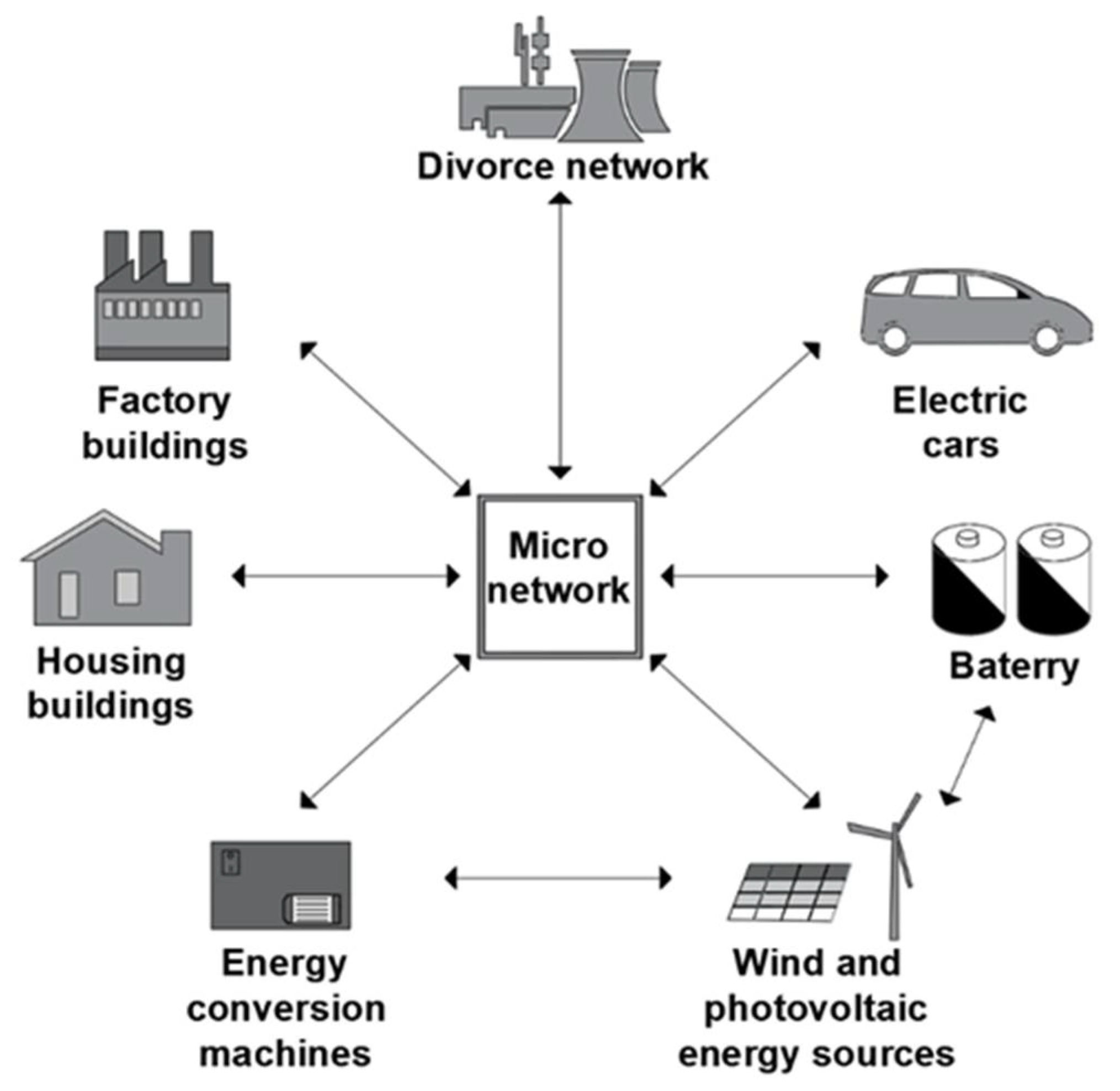
Design of RES microgrid. A microgrid is a small network of electricity users with a local energy source, which is usually connected to the national central network, but is able to operate independently. RES simulation is applied using the HOMER software (Hybrid Optimization of Multiple Energy Resources).

4th area:

Design of a photovoltaic power plant (PV) using the PV*SOL simulation program. It involves the design of PV panels in a given area, the design of inverters, the determination of the annual electricity consumption distribution of the given buildings and an assessment of the need to install battery storage in the given locality.

5th area:

Monte Carlo simulation. This is a stochastic heuristic class of algorithms for simulating systems using pseudo-random numbers. The simulation results were produced using the Palisade @Risk 7.6 simulation program, which is a Microsoft Excel add-in application. Results such as arithmetic mean, minimums, maximums and percentage quantiles are presented.

6th area:

Within our BEM, we build the infrastructure for electromobility (charging stations in a defined area), install automation and monitoring elements of the distribution network and effectively connect it to the network with local production of electricity from RES.

7th area:

Conclusion and evaluation of the research and experiment.

Benefits of the proposed BEM for the practice and its further development:

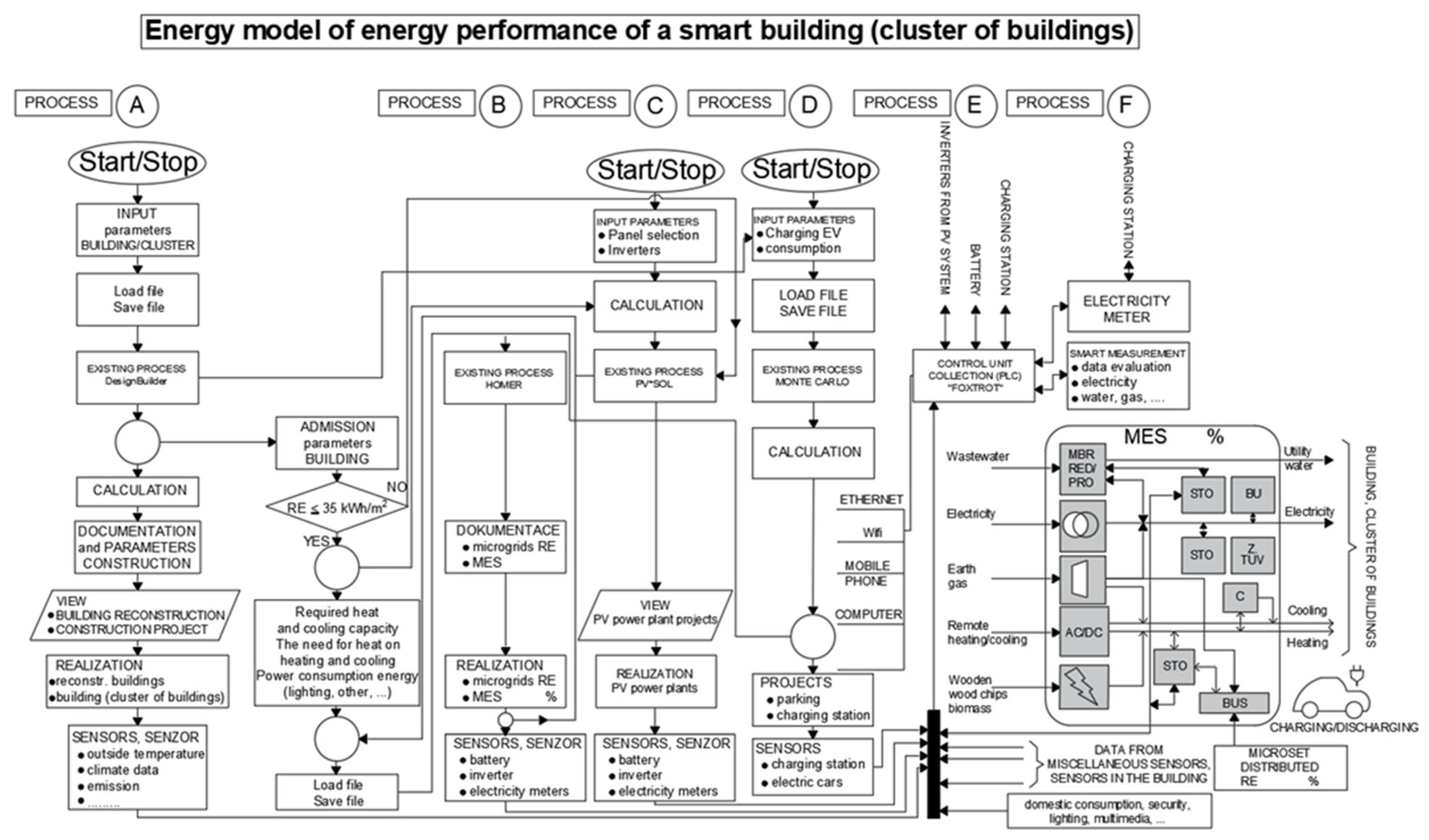
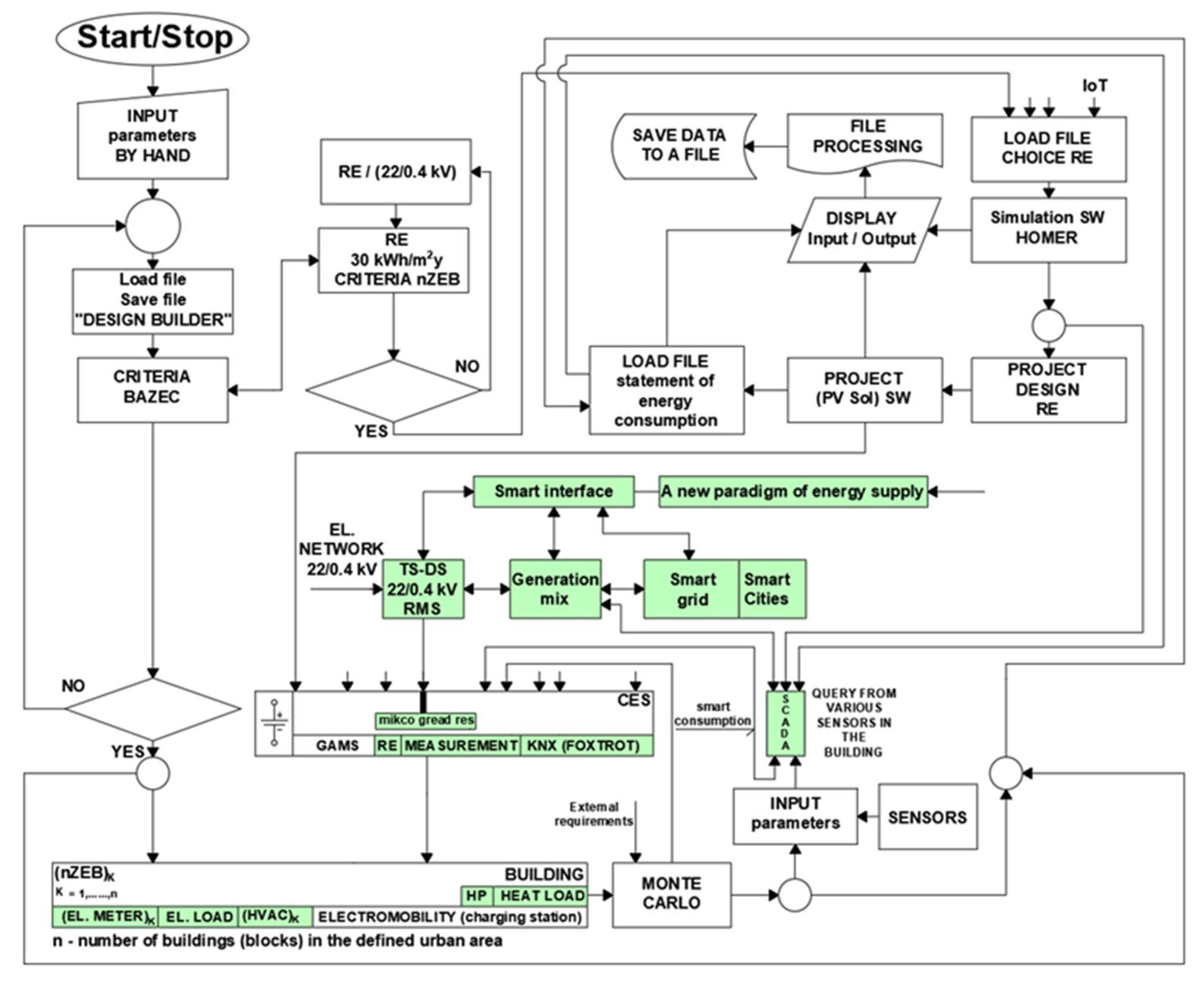
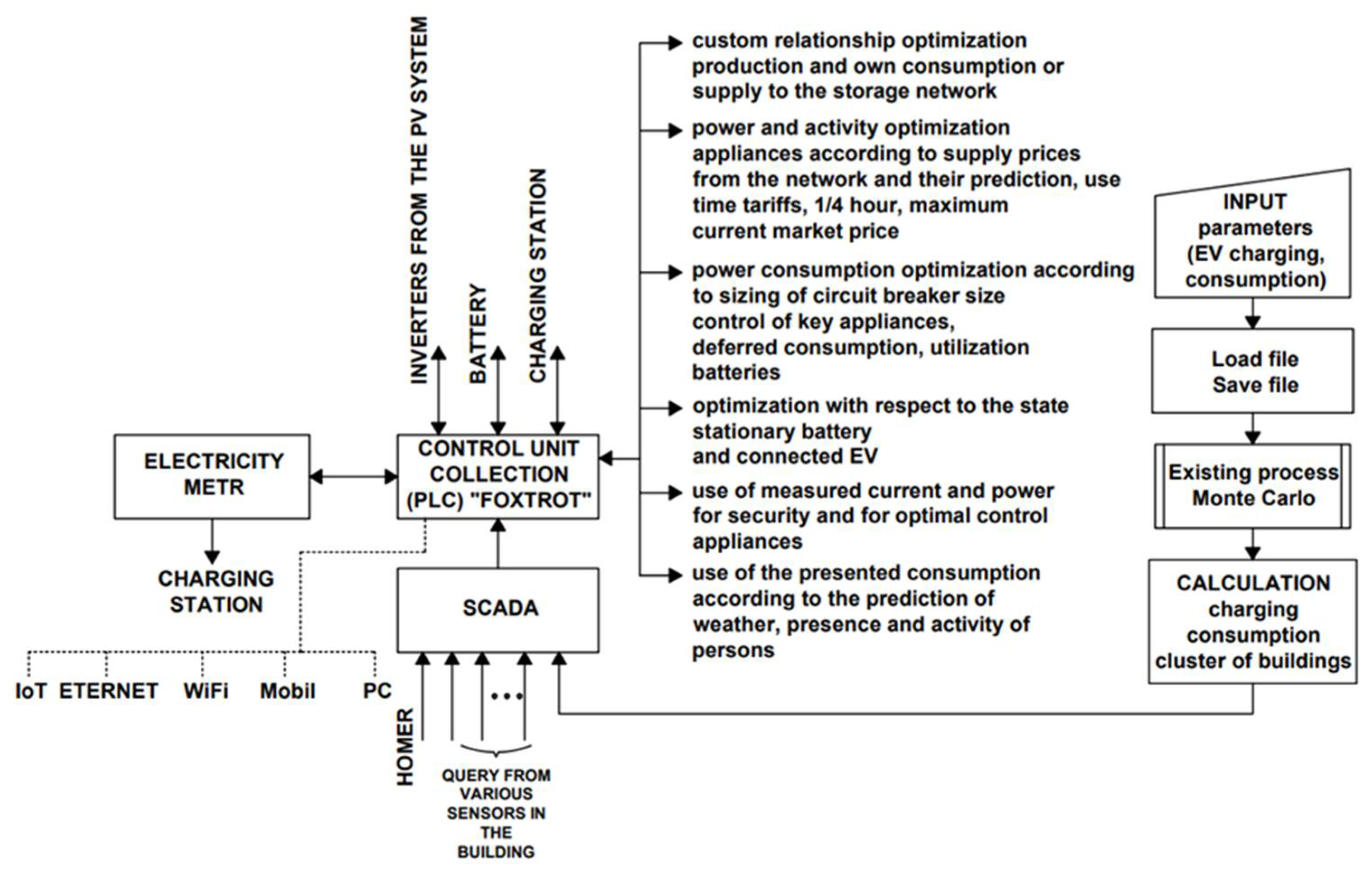
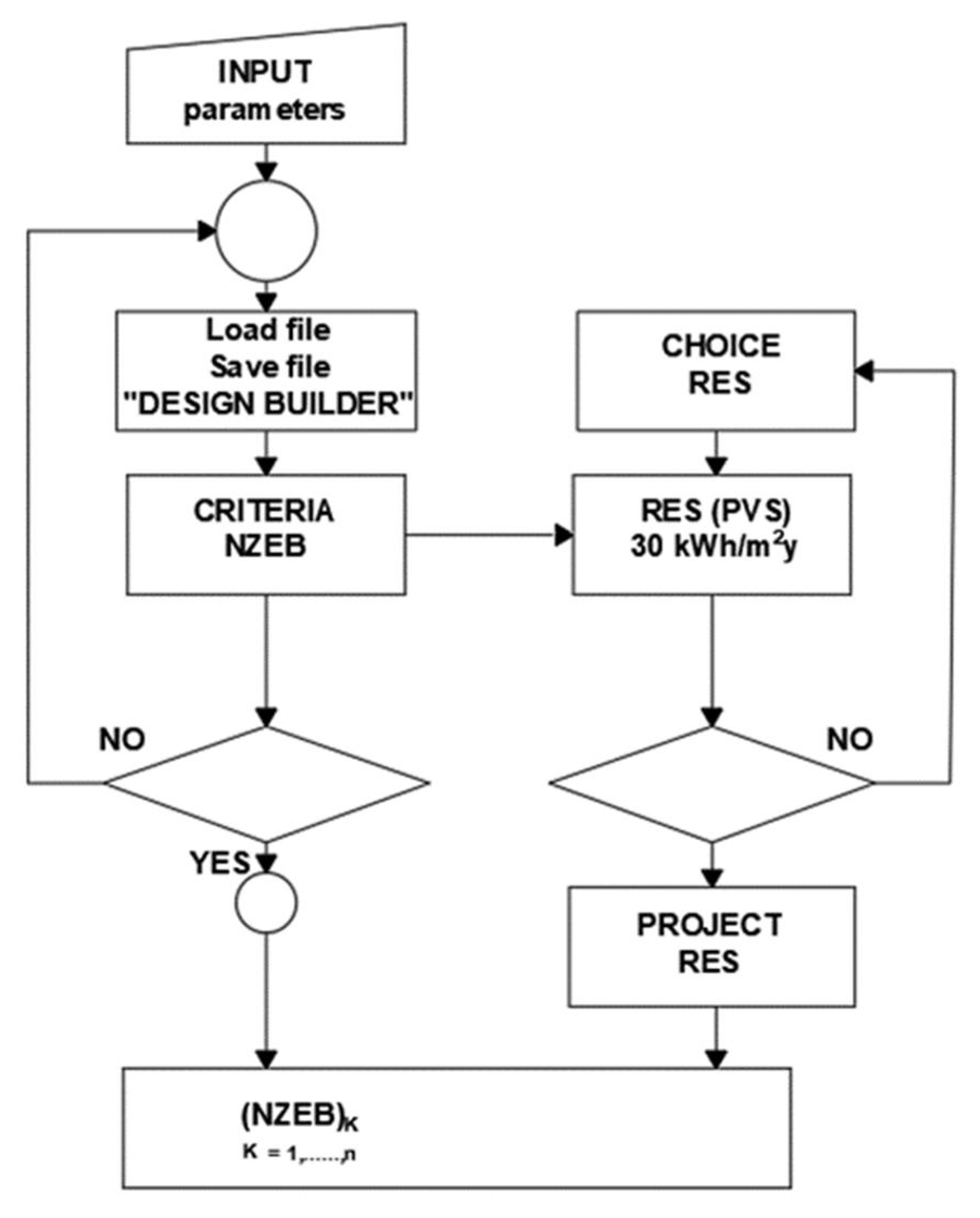
• The first factor, which we consider to be original, is the building of the system structure (system solution) of the BEM (Figure 2); its process was built based on an analysis and synthesis of simulation models.
  Figure 1 and Table 1 and

  Table 2. Normative values of the heat transfer coefficient (ČSN 73 0540-2: 2011 Thermal protection of buildings—Part 2: Requirements).

  Structure Description	Heat Transfer Coefficient (W/(m2·K))
  	Required Values UN,20	Recommended Values Urec,20	Recommended Values for Passive Buildings Upas,20
  Outer wall	0.30	Heavy: 0.25 Light: 0.20	0.18 to 0.12
  Flat and sloping roof with a slope up to 45° (inclusive)	0.24	0.16	0.15 to 0.10
  Floor and wall of the heated space adjacent to the ground	0.45	0.30	0.22 to 0.15
  Windows and doors in the external wall and steep roof, from the heated space to the outside environment	1.5	1.2	0.8 to 0.6

  show the methodological procedure of the current (existing) EPB solution in the context of NZEB buildings. The basic structure of Figure 1 is a flowchart that represents a workflow, process, system or computer algorithm. It displays the individual process steps in sequential order.

The specific selection of simulation models suited to the given issue is presented in

Table 3. Six Sigma principles. Example of a solution in our experiment.

Question	Six Sigma Phase	Description
What is this about?	Defining e.g., CO2 reduction	Define the strategic issue to be addressed. e.g., Develop NZEB project documentation
Where is the process now?	Measurement e.g., Preparation of the Energy Performance of Buildings Certificate (EPBC)	Measure the current performance of the process to be improved. e.g., An EPBC will be prepared.
What are the causes?	Analysing e.g., Analysing software tools for RES application. The electricity consumption of buildings, transport, and parking is affected. Impact on CO2. It is also necessary to address the issue of energy consumption within the EV charging process.	Analyse the process in order to identify the root causes of poor performance. e.g., The RES will be designed, as set out in Decree No. 78/2013 Sb., i.e., it is a RES design without further context and links to the actual design system with the objective for the year 2030. The most appropriate method for optimization and design of the charging system is the MONTE CARLO method.
What can be done for this?	Improving Design of a new energy model of a building on the NZEB platform in the context of sustainable energy within the Smart City concept.	Improve the process by exploring and studying possible solutions to achieve a robust improved process. The entire NZEB design and engineering process can be improved by exploring and studying possible solutions to achieve a robust improved process. Design a new methodology for designing EPB in the sustainable energy process within the Smart City (area) concept. This is to meet the key objective for 2030; see the description under the “Analysing” section.
How to maintain the achieved condition?	Managing Application of control systems for building automation. Energy savings in the range of 11 to 31%.	Standardize the improved process so that it can be managed and continuously improved to maintain its performance. This process is about standardising an improved EPB process so that it can be managed and continuously improved to maintain its performance in terms of sustainable energy. Building automation systems must be used to ensure this.

with a dynamic framework so that they interact with each other, work together, and form the structure of the so-called BEM or cluster of buildings in a given urban area. The BEM design methodology and the project and methodological quality management of the project are based on the Six Sigma application.

An important factor of a Six Sigma project is that the process be clearly structured and defined in its basic parameters such as its scope, volume, objective and structure as well as project leadership, organization, and management. A fundamental element of the quality improvement effort is the pursuit of incremental process improvement (e.g., in the form of Kaizen—change for the better) that is easily documented and measurable. The specific results of EPB in the application of BEM will be expressed in the final evaluation of the implemented building cluster project within our experiment.

Note: Design and implementation companies can continuously implement policy requirements into this energy model through directives, decrees or laws of the Czech Republic (and also the EU), including implementing documentation.

2.

The second factor is the Smart Grid application within the BEM structure. The motivation is the fulfilment of the energy sustainability platform. This makes the BEM application more original, as it strongly supports the goal of reducing energy consumption and thus CO₂ production.

2. Materials and Methods

2.1. Field of Research

2.1.1. Evaluation of EPB, Analysis of the Current State of Building Modelling and Design

Building performance simulation (BPS), known in the Czech Republic as building energy simulation (BES), is a replication of building performance (BP) aspects using a computer mathematical-physical model developed on the basis of basic physical principles and actual engineering practice.

The aim of the simulation is to quantify aspects that are relevant to the design, construction, operation and management of buildings [16]. Based on the analysis of a number of possible available simulation tools, the simulation tools listed in Table 3 were selected using synthesis.

The simulation software Design Builder (DB) [17] was then selected. It proved to be the most suitable for our application.

Design Builder is a software for complex dynamic building modelling, analysis and environmental assessment. The purpose of DB is a solution of EPB at the level of the calculation of the consumption of all energy applied in the building. The resulting building model can be imported from other BIM programs. DB software is based on the Energy Plus simulation algorithm [18].

DB input data include heat loss, solar energy, room temperature, amount of energy needed for heating, ventilation, air conditioning and lighting. All this information can be displayed in various ways, e.g., as a graph, table and the like. Other uses of DB software include, for example, evaluation of the building facade in terms of overheating, energy consumption in the building, determination of the rate of electricity savings in the building, visualization, thermal simulations, etc.

2.1.2. EPB Design Methodology and BEM Design for Sustainable Energy

In designing a new methodology for designing smart NZEB buildings within the framework of sustainable energy and the smart city, we began from the current model—see Figure 1. Finally, the “Design Quality Management Methodology based on Six Sigma” [19] supports the design of the new methodology. A fundamental element of the quality improvement effort is the effort to incrementally improve the processes (e.g., in the form of Kaizen) change for the better), which is easily documented and measurable (https://digilib.k.utb.cz/bitstream/handle/10563/22513/jedlitschka_2012_dp.pdf?sequence=1, Aleš Jedlitschka, Diploma thesis: Use of Kaizen method, accessed on 18 May 2012). Selecting the right project that fits measurable criteria (e.g., we should produce 40% less greenhouse gas in 2030 compared to 1990, etc.) with easily definable units of measurement [20] is also an integral condition for future success. We proceeded by setting the (EMB) project design priorities according to a strictly defined methodology, based on the Six Sigma tool. We asked ourselves the following questions:

• Does the potential project have the character of recurring phenomena?
• Are there appropriate metrics? If not, can metrics be established within an appropriate time period?
• Is it possible to manage, i.e., control the process?
• Will the potential project improve customer satisfaction?
• Is the potential project linked to at least one business metric (indicator)?
• Will the potential project generate savings?
• Does the potential project have a high probability of completion when applying the DMAIC method within six months of its start? (DMAIC stands for Define, Measure, Analyse, Improve and Control. At each stage there are a number of useful methods and tools.
• Can “success” criteria be established for this project?

If the answer to the above questions is “YES”, the potential project should be considered suitable for implementation. The specific activities in the Six Sigma methodology projects can be summarised in the following points:

• Data collection.
• Obtaining information from the data by analysing it.
• Proposing solutions.
• Ensuring that the desired results are achieved.

The Six Sigma principle is presented in Table 3.

2.1.3. Final Evaluation of the Six Sigma Principle and BEM Design

An essential impact of projects based on the Six Sigma principle is the area of cost savings [21]. The more an organization (design company, etc.) invests in the quality preparation of project documentation and the subsequent supervision of compliance with its design, as well as in good planning and operational interdisciplinary controls, the greater the savings of excess costs it can achieve. Therefore, it is nonsense to assume that project quality and its implementation is expensive; it is the redesigns, corrections, additions and waiting for additional required information that are expensive.

Based on the evaluation of the Six Sigma principle, an analysis of simulation tools for EPB was prepared. Table 3 shows the reference and normative values of the EPB. Table 1 and Table 2 summarizes the analysis of simulation tools for the selection of software suitable for the application of the selection and optimized design of charging stations for RES and electromobility. Using the simulation results shown in

Table 4. Synthesis of model approaches for RES solutions within a building cluster [22].

	Infrastructure	Presence of RES	Simulation and Control	Time Step Simulation
MESCOS	Electricity, heat	Yes	Yes (comprehensive)	Sec
CITYSIM	Heat	Yes	No	After hours
ENERGY PLUS	Heat	Yes	No	Minutes
ENERGY PLAN	Electricity–Heat-Transport	Yes	Yes (after simple)	After hours
HYBRID2	Electricity	Yes	Yes (comprehensive)	5 minutes
GRID-LAB	Electricity (detailed)	Yes	Yes (comprehensive)	Parts of seconds
RETSCREEN	Electricity (detailed)	Yes	Yes (simple)	After hours
RAPSIM	Electricity (detailed)	Yes	No	Minutes
DESIGN BUILDER	Electricity–heat	Yes	Yes	Minutes
MONTE CARLO	Electricity	Yes	Possible	Minutes
HOMER	Electricity	Yes	Yes	Minutes

and respecting the European Energy Performance of Buildings Directive (EPBD 3), the BEM shown in Figure 2 is proposed.

It is clear from the definition of systems theory that a system is a group or combination of interconnected, interdependent or integrating elements between which we distinguish their relationships and thus form a system structure or set of virtual pairs (agents) defining a collective whole, i.e., BEM. Since the EMB deals mainly with the application of variously defined simulation models (elements), the complex of elements of this model is in a certain defined interaction, i.e., it has defined inputs and outputs, which influences the behaviour of this model, i.e., BEM. The result is the fulfilment of the requirements and needs of the building(s) by their smart behaviour. Figure 2 shows the BEM, which is a basic prerequisite for creating the NZEB project documentation. To minimize energy losses, it is advantageous for the energy conversion to occur in one place. In the case of integrated community energy systems connected to energy networks, there is also a need for connection points for these networks. The so-called Energy Hub (EH) is created by a suitable connection of these connection points with a place where energy conversion or additional production takes place and where energy can also be stored, and all components can be reliably controlled. Figure 2 shows an example of the concept of the Municipal Energy Centre (MES) (Legend k Figure 2: MBR—membrane bioreactor; RED—reverse electrodialysis; PRO—pressure retarded osmosis; STO—media accumulation (electricity, heat, salt water); C—regulator; DH/DC—district heating/cooling) and the so-called Energy Hub, on the basis of which energy planning takes place at the district level (cluster of buildings, premises, city districts, etc.). EH is part of the external intelligence of buildings.

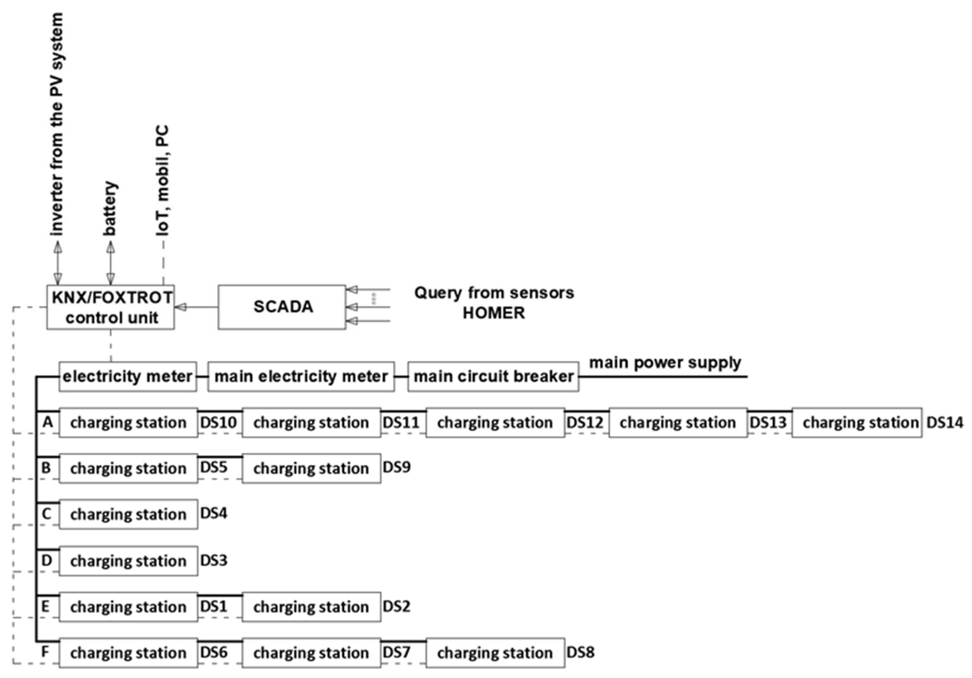
2.2. Smart Grid and Building Energy Model (BEM) Structure

It is obvious that we are increasingly focusing on obtaining energy from RES. It is a logical path that has the fundamental goal of achieving energy self-sufficiency in conjunction with energy sustainability. If we want to use this process effectively, we must develop a new concept of both transmission and distribution systems. This is a smart grid design—Smart Grids (SG). The essence of this new Smart Grid [22] is a communication infrastructure that connects energy producers and consumers. In other words, it is a two-way exchange of information and energy between producers and consumers. This is the basic principle of the smart grid at the level of balancing local surpluses and energy shortages. This process underlines the importance of the demand and supply management system, which we can imagine under the implementation process of unit commitment.

We define SG as a network that has additional capabilities, where network failures can ensure their automatic correction.

Another important application is cloud services. For active cloud applications, SG collects data from all installed types of meters at regular intervals and the customer has immediate access to them online. We can measure the consumption of electricity, heat, water and gas, but the SG system can also communicate with sensors for measuring temperature, humidity, CO₂ and other devices. It is also connected to a network of weather stations. The customer can recalculate energy consumption per m² of floor space or one person in the building at any time in the application. This feature is very important in the process of solving the energy performance of buildings (EPB), because it warns of possible wasted energy. An SG energy control scheme was developed using Lyapunov optimization theory, which can dynamically solve a problem at any point in time based on the current state of the system (https://ieeexplore.ieee.org/abstract/document/5596726; Conference date: 18-23 July 2010, DOI: 10.1109/IJCNN.2010.5596726, accessed on 19 January 2022). Smart Grid is implemented in two steps.

• The first step is to provide control and management of local inverters or photovoltaic grid inverters (on grid) so as to make them suitable for electricity storage, and to monitoring and control applications. This is done through the distributed management system (DMS) of these so-called generators.
• The second step is to provide voltage control.

The management of the local energy system is based on the requirement of better information about the function of, for example, a photovoltaic system, including ensuring its reliability and efficiency. Accurate information is increasingly important in today’s challenging market situation full of deregulation.

The basic characteristic of Smart Grid is the communication capability of the device within the network. The combination of the building energy system and the communication system as such is shown in Figure 3, which forms an interconnected network.

Communication includes parts of the communication, component and information layer from SGAM (CEN-CENELEC-ETSI 2012). A conceptual model of open systems interconnection (OSI) has been developed for the classification of communication functions of telecommunication or computer systems (International Organization for Standardization/International Electrotechnical Commission 1994). It can be adapted for communication in the context of the power system, which is described in Figure 3 as BEM.

The three main classifiers for power system communication consist of information flows through an intelligent interface, a service layer, and a technological implementation secured by an intelligent SCADA/EMS network. In Figure 3 the individual modules (coloured in light green) forming the basic architecture of the Smart Grid are implemented through a basic block diagram. It shows the Smart Grid architecture used by the power company for smart measuring for homes and business premises. The Smart Grid application in the BEM structure ensures its relevance and functionality through:

• Electric Smart Grids—independent control of the electricity supply depending on a reduction or increase in consumption;
• Smart meters installation—transmission of consumption information;
• Smart interface—timely combination of the use of electrical appliances and distribution of electricity according to need, which significantly reduces energy costs.

Figure 2 shows a city energy centre or “Multi-Energy System” (MES). It is a logical system that represents the combined processes of obtaining and using energy to meet the needs of energy services in a given urban area. It includes a micro-network of RES as one element of a complex energy system; next to it there are cooperating elements of various energy carriers (gas, sewage, electricity from the distribution network, etc.). In this case, we are also talking about the so-called Energy Hub (EH). It is a place where the production, transformation, storage and consumption of various energy carriers takes place. It is a promising alternative for integrated MES management. The RES microgrid is a strategic element of the BEM with the implementation of SG (Figure 3).

2.2.1. Smart Grid and Complex Systems

Smart Grid is an important energy system of current energy requirements, especially in the process of energy sustainability and self-sufficiency. In this context, information and communication technology (ICT) infrastructure is an indispensable component [23], [24]. In addition, a number of new features, services and processes are emerging, which in the context of Smart Grids appear to be important as highly interoperability-oriented components that should be integrated [24]. If the growing amount of energy from RES is to be integrated and at the same time efficiency is to be significantly increased in the entire existing system, this requires major changes in the entire energy system and network structure, in particular in the way this system should be operated. TC 57 standards are very important in terms of SG concept design and implementation:

(a)

IEC TR 62357-1: 2016 Power systems management and related information exchange—Part 1: Reference architecture.

(b)

IEC 61968-61970: Power generation application integration—Distribution control system interfaces—Part 1: Interface architecture and general recommendations.

(c)

IEC 61850: a set of standards for energy communication with great potential benefits.

(d)

IEC 62351: Vertical Security for the TR 62357.

(e)

IEC 60870: Telecontrol protocols (though mostly expected to be a deprecated legacy standard).

(f)

IEC 62541: OPC UA—OPC Unified Architecture, Automation Standard.

(g)

IEC 62325: Market Communications using CIM.

(h)

ČSN ETS 300 348 Intelligent network (IN). Physical plane for intelligent network Capability Set 1 (CS1) (ITU-T Recommendation Q.1215 (1993)).

(i)

EN ETS 300 374-3 ed. 2 Intelligent network (IN)—Intelligent Network Capability Set 1 (CS 1)—Core Intelligent Network Application Protocol (INAP)—Part 3: Test Suite Structure and Test Purposes (TSS& TP) for Service Switching Functions (SSF).

The common denominator of SG’s definition is that it can intelligently integrate the activities of all users connected to it (RES as energy suppliers, consumers, or both) in order to effectively provide a sustainable economy and secure electricity supplies [25].

The first SG concept on the BEM platform is shown in Figure 3 from the point of view of engineering requirements for the creation of an EPB project for a cluster of buildings (in our case, Prague 6 Bubeneč District, Vítězné náměstí). Process integration and subsequent description of the structural model supporting SG engineering requirements is proposed.

As for the design of the phrase Smart Grid, it was first introduced by Amin in 2005 [26]. SG is an energy network that, based on qualified information, tries to predict and intelligently respond to the behaviour of electricity users and suppliers. SG aims to effectively provide reliable, energy and economic information [27]. SG has fundamental goals that provide economic, energy and social needs. They are:

• Energy reliability and efficiency.
• Energy sustainability.
• Environmental quality.
• Reducing energy consumption and CO₂ production.

To achieve these goals, advanced technologies have been developed and implemented in the energy system. These are mainly various technologies for sensing energy parameters, control methods, optimization of smart grids, intelligent communications, which have been integrated into the current energy system [28,29]. The smart grid should have the following key features:

(1)

Automatic fault protection.

(2)

Ensuring the social interest.

(3)

Ensuring cyber security.

(4)

Providing energy quality.

(5)

Introduction of various RES commodities and energy storage.

(6)

Promoting thriving electricity and community energy markets.

(7)

The possibility of implementing various energy sources with intermittent production.

Over the years, a huge distribution and energy transmission network has emerged, which is not fully managed or optimized in terms of its technological level. As we have already mentioned, the aim of making it more efficient is to integrate RES in its process. In 2010, the US National Institute of Standards and Technology (NIST) collected and formalized the requirements and vision of Smart Grids in its report, which is reported in [30]. A survey was carried out in the area of SG division, where three main directions of its development were pointed out [31]:

• Smart infrastructure.
• Smart management systems.
• Smart protection.

The smart infrastructure system is considered the basis of the Smart Grid in terms of energy, information and communication infrastructure.

The smart management system consists of a process of energy measurement and remote sensing of data that meets global standards for smart metering.

We consider full automation to be smart protection, which is the connection of a digital control and management system together with sensors (sensors) that monitor the behaviour of the network and allow for automatic resumption of operation after a possible failure.

2.2.2. Smart Grid Solution Design Process

Power distribution networks are highly complex dynamic systems that are vulnerable to a large number of disturbances during daily operation. When random disturbances occur, caused by weather or some other accidents, they rarely generate large-scale [32,33] catastrophic failures. If operational data is available in real time, it opens up the possibility of unexpected disturbances. Figure 4 shows four advanced optimization and control techniques that are essential to ensure Smart Grid performance. This is perceived as a paramount condition for accepting a Smart Grid, e.g., in our experiment.

Given that the integration of the smart grid application for the EPB solution needs to be approached as part of the new NZEB design approach, it is necessary to subject the entire building design process according to BEM to complex automation.

Comprehensive automation of building services in the BEM process includes the application of computer technology and selected software (see

Table 5. CO₂ before reconstruction.

Condition before Reconstruction (Annual Values)	CO2 Production (kg)
Block A	287,893.1
Block B	201,294.4
Block C	53,153.55
Block D	140,085.30
Block E	186,972.30
Block F	315,807.10
Total:	1,185,205.75

). This is an BEM solution through BEM, which uses new algorithms to achieve energy sustainability of building clusters and reduce energy consumption and CO₂ production.

The strategic goal for the future is energy sustainability planning together with the optimal solution of the RES microgrid.

2.2.3. Electric Vehicles, Electric Hybrids and Smart Grids

There are a number of software tools: Simulation of Urban Mobility (SUMO), Quadstone Paramics, Aimsun, SimTraffic, TSIS-CORSIM, Monte Carlo and others. We evaluated the analysis that the most suitable method of optimization and design of the charging system is the Monte Carlo (MC) method. The charging process negatively affects energy consumption, which on the other hand in terms of its reduction is a characteristic milestone for the application of its deeper solution. MC software evaluates the energy load in a given area and the way it affects the consumption of individual housing units. It also evaluates the consumption profile for groups of electric vehicles (EVs) that exhibit different properties. In our experiment, we proposed different combinations of the social and economic characteristics of users. Based on this approach, the daily EV consumption was deducted. The software then calculated the initial state of charge of each electric vehicle (EV) and the daily need for recharging. It also made it possible to take into account different types of electric and hybrid vehicles. The basic algorithm in modelling power consumption for EV is the lognormal distribution. This means that in one simulation, the daily mileage of the selected number of individual cars was simulated and the sum of the needs of these cars was noted. The simulation was performed in a trial version of @Risk 7.6 from Palisade.

Figure 5 shows the connection between the EV and the network from the connection. Electricity flows through the grid from generators (photovoltaic system (PVS), power plant) to EV end users, while unused energy flows back from the EV, as shown by the two arrows in Figure 4. At times of low demand, EV batteries can be charged and discharged due to power or demand.

2.3. Microgrid of Renewable Energy Sources

For a building (renovation) project in the selected Prague 6 urban area, which addresses the EPB according to the requirements resulting from the NZEB definition, it was necessary to find a software that could optimize the composition of energy components in the given locality based on certain data, such as electrical load. For this purpose, an analysis of the simulation tools was developed; see Table 4. This work focuses on the HOMER Pro program developed by HOMER Energy, which is one of the main programs for this particular optimization. HOMER Pro is one of the products of the American company HOMER Energy. The name HOMER stands for Hybrid Optimization of Multiple Energy Resources [35]. Thus, HOMER Pro focuses on the optimization of microgrid energy resources. The RES microgrid is part of MES in the given area of our experiment and is distributed through their sources (FVS panels) on the roofs of buildings of individual units A, B, C, D, E and F. The given RES microgrid is able to operate independently; for an example, see Figure 6.

In other words, our RES microgrid is basically a local island network that can function as a stand-alone or network system. It contains inverters according to the layout of the photovoltaic panels on the roofs of the individual building blocks, which enable their connection to the existing network. Special purpose filters are installed in the FVS, which overcome harmonic problems and at the same time improve energy quality and efficiency [36].

HOMER Pro has a primarily economical and partially engineered solution for microgrids [38]. The core of the program is a simulation model developed by HOMER Energy that incorporates all the components the user wishes to consider, and it simulates microgrid operation throughout the year. The simulation time step can range from one minute to one hour. The program further optimizes the microgrid design to determine which components are appropriate and which are not appropriate for a given area, thereby finding the option that appears to be the least costly. For its calculations, the program uses a price per unit of energy, so that it can evaluate an option where the initial cost will be higher but which will be more advantageous over time.

2.4. PV*SOL Simulation

The design of the photovoltaic power plant was solved in our experiment using the PV*SOL simulation program. The program was used to design PV panels and inverters and to determine the distribution of annual electricity consumption of the buildings and assess the need to install battery storage and charging stations for electric vehicles in the area. The program offers the possibility to choose the local system with regard to the use of the PV plant (building consumption, battery system, electric vehicles and island system).

2.5. Monte Carlo Simulation, Design of Charging Stations in the Car Park

Electric vehicles, hereafter referred to as EVs, are vehicles that use electrical energy stored in a built-in battery as fuel. The range of an EV depends mainly on the capacity of the battery. Since the automotive industry is intensively involved in the development of electric vehicles and limits the development and production of gasoline and diesel vehicles, we address the issue of charging these vehicles here.

Monte Carlo software [39] was applied to define the average simulated electricity consumption for EV charging. It is a stochastic heuristic class of algorithms used to simulate systems using pseudo-random numbers. The idea of this method is to try to determine the mean value of the quantity using a random sequence of events. Once the computer model has been built and a sufficient number of simulations have been run, it is possible to apply common statistical methods such as arithmetic mean, minimums, maximums and percentage quantiles to the results obtained. Monte Carlo methods are numerical methods for solving mathematical problems by modelling random variables and statistically estimating their characteristics. The method is based on conducting random experiments with the system model and evaluating them. The result of performing a large number of experiments is usually the probability of a certain phenomenon. Therefore, to increase the accuracy of the result by one order of magnitude, the number of simulations must be increased by at least two orders of magnitude. In other words, the accuracy of the Monte Carlo method is directly proportional to the number of iterations performed. Assuming that the random process is repeated n times, the accuracy of the result will be equal to 1/√n. Therefore, to obtain a result one decimal place more accurate, it is necessary to perform the iterations 100 times. The Monte Carlo simulation results presented in this study were generated using the Palisade @Risk 7.6 simulation program, a Microsoft Excel add-in application. The simulations were run with 1,000,000 iterations, so that the results are accurate to 3 valid digits.

2.6. Methods

Achieving the desired energy savings and CO₂ emission reduction values in our experiment was due to the project’s being based on the application of the newly designed EMB including the implementation of Smart Grid in this model (Figure 3).

Another measure to achieve energy savings and reduce CO2 emissions is the solution of frequency and active power management in order to achieve a power balance, which is a natural and currently fully acceptable process. Achieving the power balance in the electricity system can also be very positively influenced by the application of unit deployment, especially RES, as proposed in our experiment.

The company providing the energy transmission system is always responsible for maintaining the energy balance, i.e., the balance between consumption and electricity production. To achieve the balance, on the one hand, operational reserves of electricity are provided and, on the other hand, regulatory tools are used.

The transmission system operator (TSO) is committed to ensuring the quality and reliability of electricity supply in the transmission system (TS). This means maintaining the frequency and voltage in the TS at the values defined by the TS Code and guaranteeing continuity of the supply at the points of consumption. The basic prerequisite for the aforementioned conditions is to maintain a balance between production and consumption, i.e., to secure the missing power when consumption exceeds production or to reduce production or secure consumption when the opposite is the case. TSOs must therefore have a certain amount of standby control power available, which they must reserve on the basis of contracts with individual providers, i.e., electricity producers. Services reserved in this way are called ancillary services (AS). The individual ancillary services are primary frequency control of the unit, secondary power control of the unit, operating reserve for t minutes (t = 5, 15, 30 min), power reduction, secondary voltage and reactive power control, island operation capability and black-start capability.

For power balancing services, the flexibility of power plants, heating plants and the consumption side are currently used, i.e., increasing or decreasing their production or consumption on instruction from the dispatching centre. The TSO has been testing for some time the possibility of extending the power services market by other actors such as smaller sources, battery systems or smaller consumers. The role of the TSO’s dispatching centre is to compensate for momentary deviations between production and consumption. Every few seconds (4 s in the Czech Republic), the deviation of the active power transmitted to neighbouring systems from the planned value is measured and, after the correction for the deviation of the network frequency, this deviation enters the central f and P controller. The output of this controller is the desired power values of the units providing the auxiliary service of the secondary P control.

Maintaining the power balance in real time is a matter of physical and technical aspects with the responsibility of the TSO as a system service. In an interconnected ES, the power balance is given by the following equation (see, e.g., [32]):

$${\displaystyle \sum }{P}_{EB}={\displaystyle \sum }{P}_{SP}+{\displaystyle \sum }{P}_{ZT}$$

(1)

• ${\displaystyle \sum }{P}_{EB}$ is the sum of active outputs supplied by the generators,
• ${\displaystyle \sum }{P}_{SP}$ is the sum of the ES active load, including the plants’ own consumption and user consumption,
• ${\displaystyle \sum }{P}_{ZT}$ is total losses in grids.

Every time this balance (1) is disturbed, the frequency and voltage of the network changes. This change will continue until the power balance is restored [40]. The power balance in the system is valid only for certain values of frequency and voltage in the system. When they change, the power produced (consumed) changes. This also applies vice versa, when the power supplied or the load in the system changes, the frequency and voltage change. It should be noted that Equation (1) is valid at the level of the whole interconnected system. he two sums in Equation (1) also change due to [40]: random load fluctuations (Figure 7); trend changes related to the shape of the daily load chart; unit outages; unregulated supplies (e.g., from wind turbines); changes in the offer during business hours breaks.

The control of $f$ and $P$ has a hierarchical character. The basic level is the primary control implemented at the power unit level. This is followed by secondary control of $f$ and $P$. For the primary frequency control, the following applies:

$$dP={\displaystyle \sum }{P}_{EB}-{\displaystyle \sum }{P}_{SP}-{\displaystyle \sum }{P}_{ZT}-P_{PLAN}$$

(2)

• ${\displaystyle \sum }{P}_{EB}$ is the total active power supplied by the generators of the control area,
• ${\displaystyle \sum }{P}_{SP}$ is the sum of the active load of the control area, including the plants’ own consumption and user consumption,
• ${\displaystyle \sum }{P}_{ZT}$ is the total losses in the control area,
• $P_{PLAN}$ is the planned balance of transmitted power of the control area (positive $\Delta P_1$ for exports and negative $\Delta P_2$ for import),
• $dP$ is the balance deviation.

If the power of the control area is small compared to the power of the whole interconnected ES, then $dP\cong \Delta P$ is approximately true. Energy exchanges (import/export) must be maintained at the planned agreed value of $P_{PLAN}$ [41], which is primarily the task of secondary frequency and power management.

Secondary frequency and power control is automatically provided by the secondary frequency and power controller, including the Area Control Error ($ACE$). The $ACE$ is calculated as follows:

$$ACE=\Delta P-K\Delta f$$

(3)

ΔP—the deviation of transmitted power from the planned value: the difference between the instantaneous sum of the measured power flows at the border between the transmission and distribution system and the planned power balance (in this sense they correspond to positive values for imports, in contrast to the $P_{PLAN}$ value in Equation (2)).

K—set parameter of the controller (the so-called K-factor), which should theoretically be equal to the power number of the control area, and which is determined similarly to the total primary control reserve in proportion to the amount of electricity produced annually).

The caused power imbalance, manifested by the frequency change and the deviation of the transmitted power, is compensated only by the control (where the power imbalance occurred) and at the same time the controller of the unaffected area does not regulate the power deviation caused by the primary frequency f control. We can see this by a simple consideration. If we substitute the summary change in turbine power according to Equation (2) for ΔP in Equation (3), taking into account the sign convention, which is positive for imports (we neglect the load control effect for simplicity), then we get:

$$ACE={\displaystyle \sum }{K}_P\Delta f-K\Delta f=\Delta f({\displaystyle \sum }{K}_P-K)=\Delta f\left(K_{SYS}-K\right)=0$$

(4)

When the power numbers $K_{SYS}={\displaystyle \sum }{K}_P$ and the $K$-factor are the same, the area control error ($ACE$) is zero. Power balance is restored by secondary frequency and power control and primary frequency control to gradually replace the power provided on a solidarity basis in the interconnected system, and secondary frequency and power control should restore the specified frequency and power values within 15 min after the emergence of power imbalance. The secondary frequency and power control is followed by tertiary power control, which serves to replace the depleted secondary control reserve, i.e., the power consumed in the secondary control activity. For tertiary management, the spinning reserve is used at units providing the tertiary performance management support service.

3. Results of the Experiment

3.1. Application of Simulation Models in EPB Solutions

The selected simulation software (Design Builder), which will be presented subsequently, was applied for modelling the energy performance of buildings (EPB). These are buildings in the urban area of Prague 6 Bubeneč (cluster of buildings). The selected area was subjected to an experiment. In the experiment, we marked the individual buildings (cluster of buildings) with the letters A, B, C, D, E and F (see Figure 8).

The given blocks were modelled in two variants before reconstruction (without insulation, heat source as gas boilers, conventional ventilation and insulated hot water pipes) and after the reconstruction (with insulation, heat source as gas boilers, photovoltaic plant, LED lighting and insulated hot water pipes).

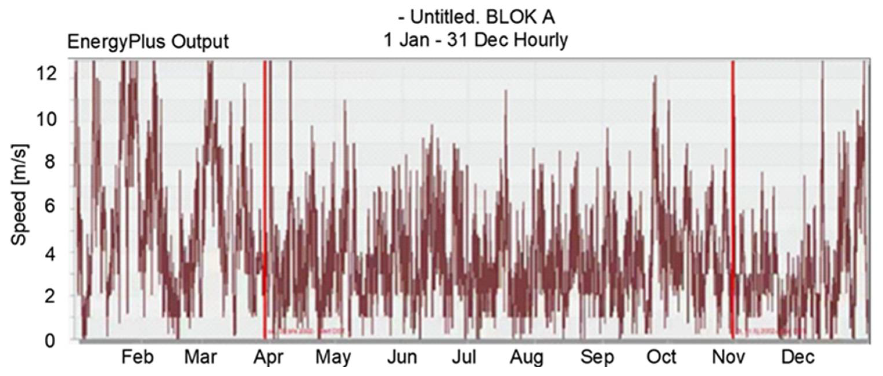
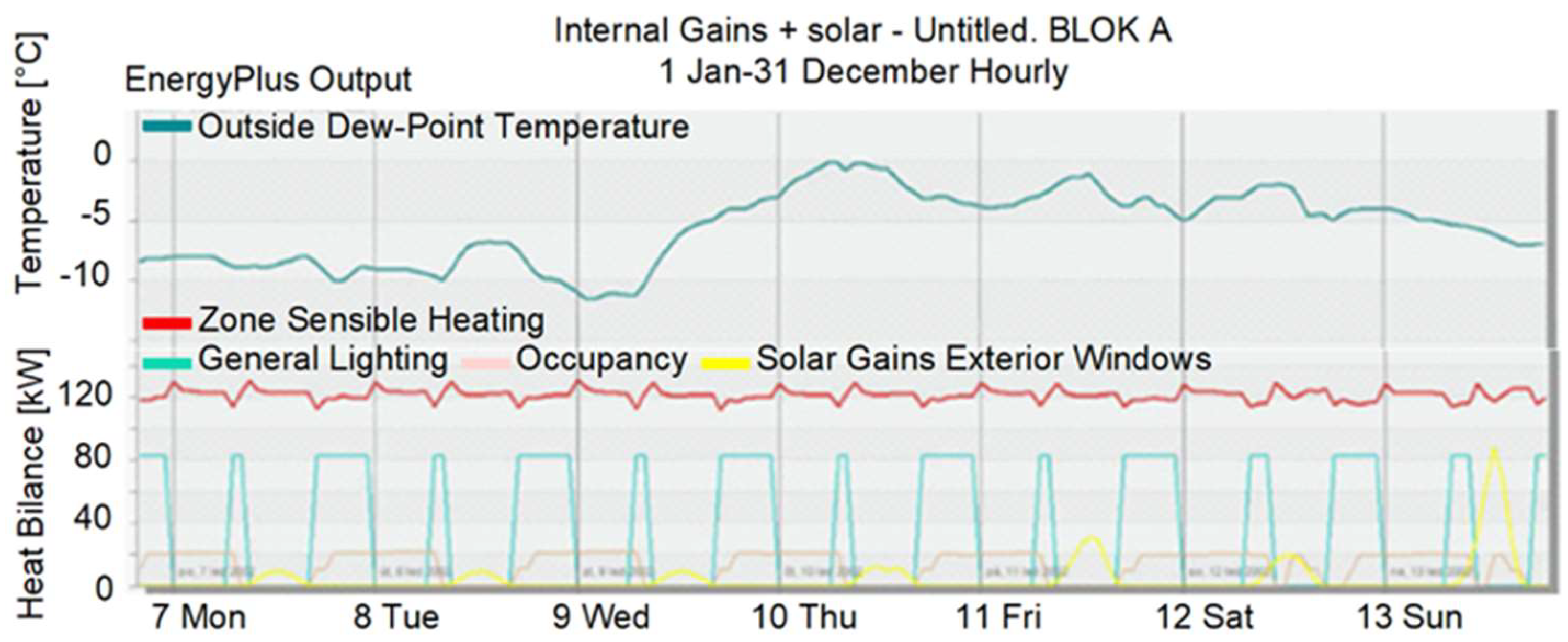
3.1.1. Design Builder—Climatic Data

We first chose the locality and orientation of the building. Then, we obtained the outdoor temperature in that locality (Figure 9), the wind speed (Figure 10) and the direct and diffuse radiation (Figure 11). All these inputs affect energy consumption.

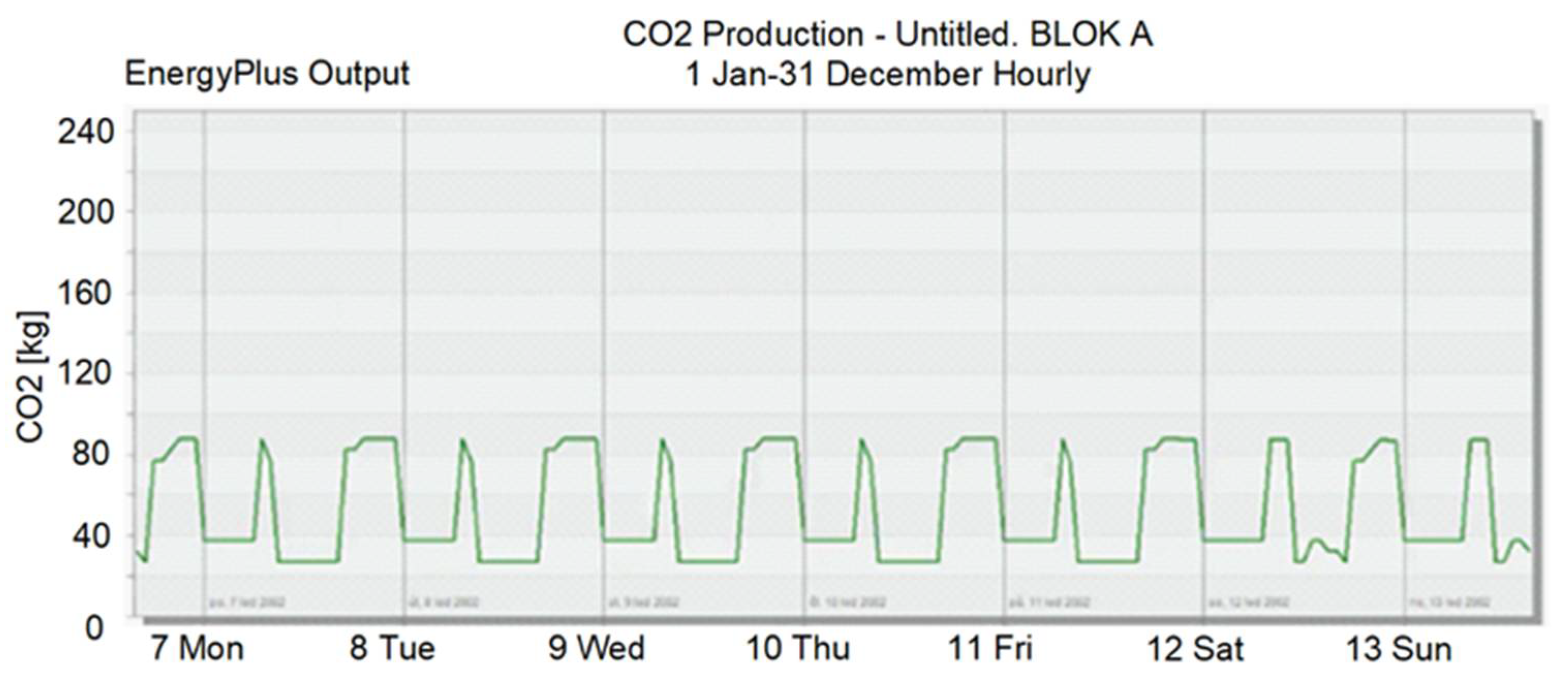
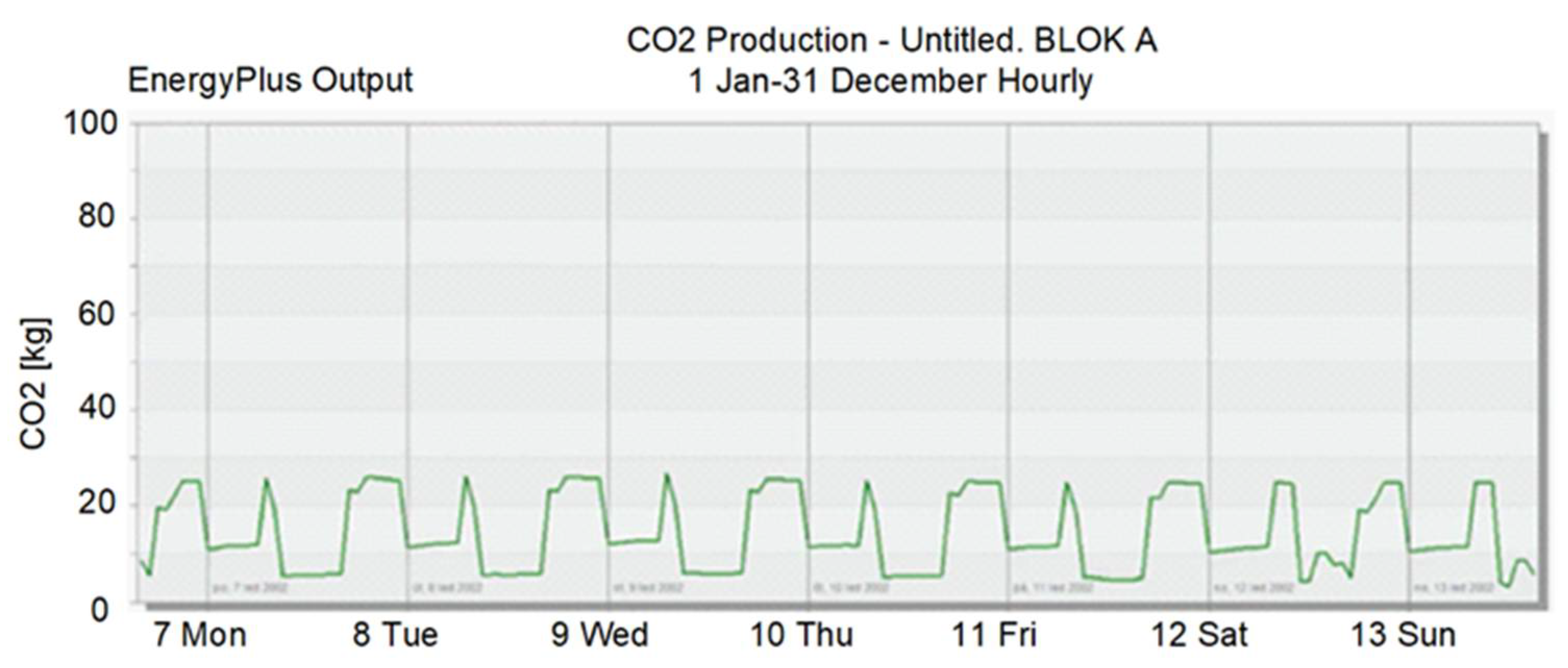
3.1.2. CO2 Production

Based on the simulation, the annual CO₂ production was determined for the objects solved in the urban area. The reduction of CO₂ production was achieved by insulating the buildings and adding a photovoltaic plant to the existing source (to the gas boilers) as part of the RES microgrid. Figure 12 and Figure 13 and Table 5 and

Table 6. CO₂ after reconstruction.

Condition after Reconstruction (Annual Values)	CO2 Production without PV (kg)	CO2 Production with PV 1 (kg)
Block A	87,472.45	409.45
Block B	54,098.88	25,951.88
Block C	13,406.89	9015.89
Block D	41,359.04	10,339.04
Block E	47,204.16	8829.16
Block F	80,969.36	42,482.36
Total:	324,510.78	97,027.78

¹ PV denotes a photovoltaic power plant.

show its behaviour and the reduction in CO₂ production for the condition prior to the reconstruction and subsequently after the reconstruction.

For the condition after the reconstruction, the table was divided into two parts, namely CO₂ production only with insulation and without a PV plant on the one hand, and the CO₂ production with both insulation and a PV plant on the other. Thanks to these param-eters used, the buildings were close to the group of buildings with nearly zero energy consumption.

3.1.3. Heat Demand for Heating

A significant factor affecting energy performance is the heat demand for heating. Reducing the heat demand for the urban area in question is achieved by selecting building structures with the required heat transfer coefficient values, and it is the heat transfer coefficient that is one of the indicators that assesses whether a building is an NZEB. The values of the specified heat transfer coefficients are given in

Table 7. Determined heat transfer coefficients for given building blocks.

	Condition Before Reconstruction	Status	Condition after Reconstruction	Status
Uwall	1.1	Not suitable	0.21	Satisfies
Ufloor	1.03	Not suitable	0.26	Satisfies
Uroof	1.1	Not suitable	0.18	Satisfies

. The values of the required heat transfer coefficients according to the legislation are given in Table 2. The reduction is also affected by gains from people, lighting, technology and solar gains. Heat demand trends and values are recorded in Figure 14 and Figure 15 and

Table 8. Heat demand before reconstruction.

Condition before Reconstruction (Annual Values)	Heat Demand for Heating (kWh)
Block A	518,829.6
Block B	431,060.1
Block C	124,580.9
Block D	324,022.8
Block E	416,312.1
Block F	766,314.1
Total	2,581,119.6

and

Table 9. Heat demand after reconstruction.

Condition after Reconstruction (Annual Values)	Heat Demand for Heating (kWh)
Block A	2295.01
Block B	10,319.52
Block C	7407.81
Block D	6690.62
Block E	10,278.40
Block F	15,768.51
Total	72,559.87

.

3.1.4. Energy Consumption

The DB software was used to simulate individual consumption for the whole year, which is another indicator of whether it is an NZEB. The simulated energy consumption included consumption of electricity, heating and hot water. The values and sample behaviour are shown in Figure 16 and Figure 17 and

Table 10. Power consumption before the reconstruction.

Condition before Reconstruction (Annual Values)	Electricity (kWh)	Heating (kWh)	Hot Water Preparation (kWh)
Block A	164,585.2	609,859.2	315,617.0
Block B	122,803.2	506,729.8	198,661.1
Block C	38,476.8	146,461.6	28,767.39
Block D	91,296.0	381,097.4	135,167.5
Block E	128,563.2	489,506.9	124,050.3
Block F	183,859.2	901,178.3	244,249.3

and

Table 11. Power consumption after the reconstruction.

Condition before Reconstruction (Annual Values)	Electricity (kWh)	Heating (kWh)	Hot Water Preparation (kWh)
Block A	62,503.9	24,459.7	239,962.9
Block B	38,572.8	9746.4	154,061.4
Block C	11,140.6	8388.2	27,097.4
Block D	27,545.9	6430.7	125,080.5
Block E	38,771.3	11,078.0	115,328.4
Block F	55,984.8	15,928.8	234,884.8

.

3.1.5. Primary Energy

The last indicator is primary energy consumption per year.

Table 12. Values of conversion factors.

Energy Carrier	Conversion Factor f (Primary Energy Factor from Non-Renewable Energy Sources) (kWh/kWh)
Natural gas	1.0
Electrical energy	2.6
Electricity-photovoltaic power plant	0.2

shows the values of the conversion factors. The resulting values for each block are recorded in

Table 13. Primary energy consumption values for the state before reconstruction.

	Item	Annual Energy Consumption (kWh)	Conversion Factor f (-)	Annual Primary Energy Consum (kWh)
		a	b	c = a · b
BLOCK A	Heating	609,859.2	1.0	609,859.2
	Electrical energy	164,585.2	2.6	427,921.5
	Hot water preparation	315,617.0	1.0	315,617.0
	Total	1,090,061.4	–	1,353,397.7
BLOCK B	Heating	506,729.8	1.0	506,729.8
	Electrical energy	122,803.2	2.6	319,288.3
	Hot water preparation	198,661.1	1.0	198,661.1
	Total	828,194.1	–	1,024,679.2
BLOCK C	Heating	146,461.6	1.0	146,461.6
	Electrical energy	38,476.8	2.6	100,039.7
	Hot water preparation	28, 767.4	1.0	28,767.4
	Total	213,705.8	–	275,268.7
BLOCK D	Heating	381,097.4	1.0	381,097.4
	Electrical energy	91,296.0	2.6	237,369.6
	Hot water preparation	135,167.5	1.0	135,167.5
	Total	607,560.9	–	753,634.5
BLOCK E	Heating	489,506.9	1.0	489,506.9
	Electrical energy	128,563.2	2.6	334,264.3
	Hot water preparation	124,050.3	1.0	124,050.3
	Total	742,120.4	–	947,821.5
BLOCK F	Heating	901,178.3	1.0	901,178.3
	Electrical energy	183,859.2	2.6	478,033.9
	Hot water preparation	244,249.3	1.0	244,249.3
	Total	1,329,286.8	–	1,623,461.5

and

Table 14. Primary energy consumption values for the state after reconstruction.

	Item	Annual Energy Consumption (kWh)	Conversion Factor f (-)	Annual Primary Energy Consum (kWh)
		a	b	c = a · b
BLOCK A	Heating	24,459.7	1.0	24,459.7
	Electrical energy	16,354.0	2.6	42,520.4
	Electricity produced by the power plant	46,159.0	0.2	9231.8
	Hot water preparation	239,962.9	1.0	239,962.9
	Total	326,935.6	–	316,174.8
BLOCK B	Heating	9746.4	1.0	9746.4
	Electrical energy	17,717.0	2.6	46,064.2
	Electricity produced by the power plant	20,865.0	0.2	4173.0
	Hot water preparation	154,061.4	1.0	154,061.4
	Total	202,389.8	–	214,045.0
BLOCK C	Heating	8388.2	1.0	8388.2
	Electrical energy	7624.0	2.6	19,822.4
	Electricity produced by the power plant	3521.0	0.2	704.2
	Hot water preparation	27,097.4	1.0	27,097.4
	Total	46,630.6	–	56,012.2
BLOCK D	Heating	6430.7	1.0	6430.7
	Electrical energy	8526.0	2.6	22,167.6
	Electricity produced by the power plant	19,038.0	0.2	3807.6
	Hot water preparation	125,080.5	1.0	125,080.5
	Total	159,075.2	–	157,486.4
BLOCK E	Heating	11,078.0	1.0	11,078.0
	Electrical energy	15,777.0	2.6	41,020.2
	Electricity produced by the power plant	23,012.0	0.2	4602.4
	Hot water preparation	115,328.4	1.0	115,328.4
	Total	165,195.4	–	172,029.0
BLOCK F	Heating	15,928.8	1.0	15,928.8
	Electrical energy	27,392.0	2.6	71,219.2
	Electricity produced by the power plant	28,610.0	0.2	5722.0
	Hot water preparation	234,884.8	1.0	234,884.8
	Total	306,815.6	–	327,754.8

. They are then compared to the primary energy requirement. The comparison is made in

Table 15. Primary energy consumption and coverage from RE for the state before reconstruction.

BLOCK	Usable Area of the Block (m2)	Annual Primary Energy Consumption (kWh)	Primary Energy Consumption per Year (kWh/m2)	Required Primary Energy Consumption per Year (kWh/m2)	Status	Energy Produced Renewable Resource (kWh)	Coverage of RE per Year (kWh/m2)	Required Coverage from RE per Year (kWh/m2)	Status
-	a	b	c = b/a			d	e = d/a
A	4577.6	1353, 397.7	295.7	50–65	Does not meet	No RES	No RES	35	Does not meet
B	3411.2	1024,679.2	300.4	50–65	Does not meet	No RES	No RES	35	Does not meet
C	1068.8	275,268.7	257.5	50–65	Does not meet	No RES	No RES	35	Does not meet
D	2536.0	753,634.5	297.2	50–65	Does not meet	No RES	No RES	35	Does not meet
E	3571.2	947,821.5	265.4	50–65	Does not meet	No RES	No RES	35	Does not meet
F	5107.2	1623,461.5	317.9	50–65	Does not meet	No RES	No RES	35	Does not meet

and

Table 16. Primary energy consumption and RE coverage for the state after reconstruction.

BLOCK	Usable Area of the Block (m2)	Annual Primary Energy Consumption (kWh)	Primary Energy Consumption per year (kWh/m2)	Required Primary Energy Consumption per year (kWh/m2)	Status	Energy Produced Renewable Resource (kWh)	Coverage of RE per year (kWh/m2)	Required Coverage from RE per year (kWh/m2)	Status
	$a$	$b$	$c=\raisebox{1ex}{$b$}\!\left/ \!\raisebox{-1ex}{$a$}\right.$			$d$	$e=\raisebox{1ex}{$d$}\!\left/ \!\raisebox{-1ex}{$a$}\right.$
A	4577.6	316,174.8	69.1	50–65	Does not meet	102,378	22.4	35	Does not meet
B	3411.2	214,045.0	62.7	50–65	Satisfies	33,262	9.8	35	Does not meet
C	1068.8	56,012.2	52.4	50–65	Satisfies	5207	4.9	35	Does not meet
D	2536.0	157,486.4	62.1	50–65	Satisfies	36,483	14.4	35	Does not meet
E	3571.2	172,029.0	48.2	50–65	Satisfies	45,175	12.6	35	Does not meet
F	5107.2	327,754.8	64.2	50–65	Satisfies	45,440	8.9	35	Does not meet

* The values for the required primary energy per year and the values for the required coverage from RES per year are given in Table 1.

. For the houses in question (all building blocks in the above-mentioned urban area), natural gas (heating and hot water) and electricity are used as energy carriers. For these energy carriers, we used the conversion factor values according to Table 13.

3.1.6. Comparison of Primary Energy and Coverage from RES

The following Table 1, Table 15 and Table 16 show a comparison of primary energy consumption and coverage from renewable energy sources with the required values.

3.2. Monte Carlo—Electromobility

There are five parking zones in the given urban area marked P1, P2, P3, P4, P5 (see Figure 8). In

Table 17. Number of stalls and charging stations.

Parking Sign Figure 8	Number of Parking Spaces	Number of Charging Stations
P1	26	3
P2	20	2
P3	25	3
P4	5	1
P5	44	5
Total	120	14

, it is indicated for how many parking spaces parking zones are designed. The design of charging stations is based on the fact that there is 1 charging station per 10 parking spaces. From this it is already clear how many charging stations fall on each zone (see

Table 18. Allocation of charging stations.

Designation of Residential Zones	Allocation of Charging Stations
A	DS10, DS11, DS12, DS13, DS14
B	DS5, DS9
C	DS4
D	DS3
E	DS1, DS2
F	DS6, DS7, DS8

).

As a prerequisite for the simulation of consumption in the charging stations, we determined how the charging stations would be used. In our case, each charging station was occupied by one car during night hours (20:00–6:00), mainly by the inhabitants of the residential buildings, and during the day (6:00–20:00) at least two cars took turns at each charging station. This simulated the consumption of the charging stations. We used the Monte Carlo simulation method. The theoretical consumption of the charging stations was determined by setting the demand equal to the total number of fully discharged batteries in the vehicles multiplied by the frequency of car visits during the day (see

Table 19. Simulated and theoretical consumption of charging stations.

Designation of Residential Zones	Simulated Consumption of Charging Stations (kWh)	Theoretical Consumption of Charging Stations (kWh)	Savings
A	57,613	164,250	64.92%
B	22,664	65,700	65.50%
C	11,141	32,850	66.09%
D	11,865	32,850	63.88%
E	23,581	65,700	64.11%
F	33,984	98,550	65.52%
Total	160,848	459,900	65.03%

).

Example of calculation of theoretical consumption for charging station of residential zone A:

• X—the number of charging stations for the residential area.
• Y—the value of the fully discharged battery (the battery capacity of the car under consideration is 30 kWh);
• Z—the number of cars to take turns at the charging station during the day.
• Z′—the number of cars to take turns at the charging station during the night.
• O—the number of days and $P=\left[X·\left(Y·Z+Y·Z^{\prime }\right)\right]·O=\left[5·\left(30.2+30.1\right)\right]·365=164 047 kW/year.$

The graph in Figure 18 shows the electricity consumption that the electric vehicle (EV) parking lot will need for the entire day, i.e., day- and night-time hours of operation. The graph shows that in 90% of the cases, the car park will need between 164.047 kWh and 193.5 kWh of electricity in total to charge all the cars. The highest consumption in the simulation was 218.35 kWh and the lowest was 147.138 kWh. Ten EVs were generated for each individual simulation.

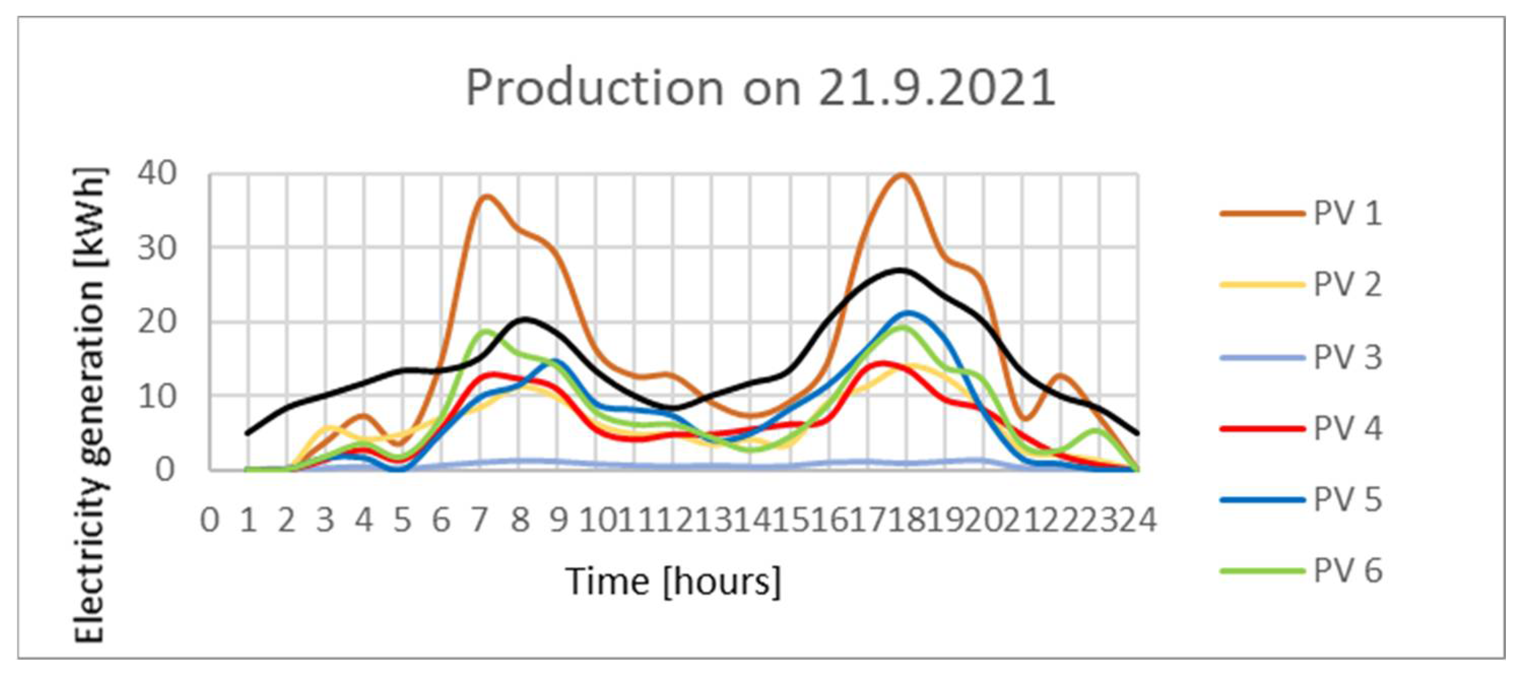
3.3. PV*SOL—Photovoltaics

In the given urban area, photovoltaic power plants PV1, PV2, PV3, PV4, PV5 and PV6 were installed on the roof structures of individual blocks A, B, C, D, E and F. The electricity generated from the plants was used to cover part of the household consumption, to charge electric vehicles, as storage in batteries (from which energy is drawn at times when it is not available from the sun) and, last but not least, the excess energy was sold to a distributor. Figure 19 shows the power generation for the day 21 September 2021. An overview of the flow of energy from power plants is also given in Figure 20 and

Table 20. Energy from photovoltaic power plants and the distribution network.

PV	Energy Produced	Module Area	Orientation	Tilt	Number of Modules	Installed Power	Own Household Consumption		Battery Power Supply	EV Charging		Network Overflow	Reduction of CO2 Emissions	Share of own Consumption	Specific Annual Revenue
							Covered PV	Covered with Battery		Covered PV	Covered with Battery
-	[kWh]	[m2]	-	[°]	[pcs]	[kWp]	[kWh]	[kWh]	[kWh]	[kWh]	[kWh]	[kWh]	[kg/year]	[%]	[kWh/kWp]
PV 1	102,378	477.2	SW	34–37	216	98.28	22,331	23,828	32,099	29,521	8541	18,428	87,063	82.0	1041.61
PV 2	33,262	161.2	S	10	73	33.21	12,370	8495	12,271	7539	3525	1082	28,147	96.7	1001.15
PV 3	5207	26.5	S	10	12	5.46	2978	543	832	962	196	434	4391	91.7	952.71
PV 4	36,483	201.0	S, E, W	29–36	91	41.41	10,109	8929	9745	7969	775	8660	31,020	76.3	880.71
PV 5	45,175	269.5	E, W	10–40	122	55.51	13,326	9686	13,096	11,095	3254	7659	38,375	83.0	813.51
PV 6	45,440	225.3	SW	10	102	46.41	17,521	11,089	15,839	10,518	4482	1562	38,487	96.6	978.72

.

Table 21. Own household consumption.

BLOCK	Power Supplied by the Distribution Network	Own Household Consumtion from the Distribution Network	Power Supply to the Battery from dis. Networks	EV Charging from the Distribution Network
-	[kWh]	[kWh]	[kWh]	[kWh]
A	36,999	16,354	1094	19,551
B	29,454	17,717	137	11,600
C	17,607	7624	0	9982
D	11,866	8526	219	3121
E	25,252	15,777	243	9232
F	46,623	27,392	247	18,985

then shows the households’ own consumption.

3.4. HOMER

HOMER Pro (Hybrid Optimization of Multiple Energy Resources) focuses on the optimization of microgrid energy sources (see Figure 6). It optimises the microgrid design to determine which components are suitable and which are not suitable for the area from a financial point of view. Other elements include, for example, emissions measurement. We were also interested in the characteristics of the electrical load, the PV system on the rooftops of the cluster of buildings, the battery storage and the connection to the 22/04 kV distribution network. The database contains model loads for different types of buildings in the given climate region. Subsequently, a window appears with a summary of the details of the load in kWh per day.

January was the month with the highest load. HOMER assumes a variable electrical load. We chose the Residence profile for our area. First, we started the simulation with the basic components and then we modified the model. We then added a connection to the central national network.

Next, we selected the renewable source we wanted to consider, i.e., solar panels. We adjusted the price to $/kW, which corresponded to the area of powerful solar panels that could supply most of the area. Then we included a 100 kW Li-Ion battery, which was relatively more expensive but of higher quality. Again, the cost was in dollars per kW/hour.

Simulation Results

The results section has two parts. The first contains analytical scenarios and the second contains optimization results. The second section contains the optimized results of the microgrid scheme. Next, it contains power generation. The program optimized the grid only for PV and central grid connection, so that we can see only these two components in the graph. The columns show the data by months. We can see that the renewable energy produced was over 68% of the total energy supplied (Figure 21).

Other tabs provide an overview of the renewable energy production at the given hour of the day (Figure 22).

In the next part we can see how much energy was bought from the central network and when. The energy obtained from the distribution network indirectly copied the production of electricity from RES (photovoltaic system).

In

Table 22. Energy bought and sold during the year, difference and price in each month.

Month	Energy Purchased (kWh)	Energy Sold (kWh)	Net Energy Purchased (kWh)	Peak Demand (kW)	Energy Charge $	Demand Charge $
January	294	182	112	2	$20.11	$0
February	223	249	−26	2	$1.82	$0
March	217	301	−85	2	$5.92	$0
April	166	353	−187	2	$13.10	$0
May	130	407	−277	1	$19.42	$0
June	112	368	−256	1	$17.93	$0
July	110	407	−297	1	$20.79	$0
August	131	428	−298	1	$20.85	$0
September	163	318	−154	2	$10.80	$0

, embedded in the graph, we can see that the energy bought, the energy sold, the difference and the price in each of the months are shown (Figure 23).

The last tab shows the emission measurements listed in

Table 23. Evaluation of CO₂ measurements.

Quantity	Value	Units
Carbon Dioxide	1.462	kg/yr
Carbon Monoxide	0	kg/yr
Unburned Hydrocarbons	0	kg/yr
Particulate Matter	0	kg/yr
Sulfur Dioxide	6.34	kg/yr
Nitrogen Oxides	3.10	kg/yr

.

4. Discussion

4.1. Final Evaluation

4.1.1. Reduction of CO₂ Greenhouse Gases

The reduction of CO₂ emissions should be at least 40% by 2030 according to EPBD3, but the requirement has been increased according to the decision of the ER Summit in December 2020 to a reduction of 55% by 2030.

Table 24. Evaluation of CO₂ production before and after the reconstruction of the urban area by DB simulations.

CO2 Production (kg)	Existing State of the Solution in the Application of EPB (DesignBuilder) (kg)	Tons of CO2	CO2 Reduction according to EPBD3 by 2030 Requirement (40%)	CO2 Reduction According to EPBD3 + Summit ER December 2020. Implementation by 2030 Requirement (55%)	Existing State/after Reconstruction (%)	Met/Not Met
Total production before reconstruction	1,193,205.75	1193.2	100	100	0	Not met
Total production after reconstruction without PVE	324,510.78	324.5	72	72	72	Met
Total production after reconstruction with PVE	97,027.78	97.027	92	92	92	Met

and

Table 25. Evaluation of CO2 production before and after the reconstruction of the urban area by DB simulations of heating and electricity consumption.

Block	Electricity (Before Reconstruction) (kW)	Electricity (Before Reconstruction) (kW)	CO2 Reduction (%)	Heating (Before Reconstruction) (kW)	Heating (Before Reconstruction) (kW)	CO2 Reduction (%)	Met/Not Met Requirement—Decrease by 55%
A	164,585.2	62,503.9	62.1	609,859.2	24,459.7	95.9	Met
B	122,803.2	38,572.8	68.5	506,729.8	9746.4	98.0	Met
C	38,476.8	11,140.6	71.0	146,461.6	8388.2	94.2	Met
D	91,296.0	27,545.9	69.8	381,097.4	6430.7	98.3	Met
E	128,563.2	38,771.3	69.8	489,506.9	11,078.0	97.7	Met
F	183,859.2	55,984.8	69.5	901,178.3	15,928.8	98.2	Met
TOTAL	729,583.6	234,519.3	67.8	3,034,833.2	76,031.8	97.4	Met

present the simulation output of the DesignBuilder (DB) software. From these tables, the values that express compliance or non-compliance with the EPBD3 and the ER/2020 summit requirements are evident. That is also the result of our experiment, which confirms the correctness of the application of the new BEM methodology.

Table 26. Evaluation of CO₂ production before and after urban area reconstruction with the installation of charging stations, by DB and Monte Carlo simulations.

Block	Electricity (Before Reconstruction) (kW)	Simulated Electricity Consumption from Charging Stations (kWh)	Electricity (after Reconstruction) (kW)	Total Electricity after Reconstruction Including Charging Stations	CO2 Reduction (%)	Met/Not Met Requirement 55%
A	164,585.2	57,613	63,503.9	121,116.9	26.4	Not met
B	122,803.2	22,664	38,572.8	61,236.8	50.1	Not met
C	38,476.8	11,141	11,140.6	22,281.6	43.0	Not met
D	91,296.0	11,865	27,545.9	39,410.9	56.8	Not met
E	128,563.2	23,581	38,771.3	62,352.3	51.5	Not met
F	183,859.2	33,984	55,984.8	89,968.8	51.0	Not met
TOTAL	729,583.6	160,848	234,519.3	396,367.3	45.6	Not met

shows the evaluation of CO₂ production before and after the urban area reconstruction with the installation of charging stations, based on the DB and Monte Carlo simulations.

4.1.2. Reduction of Energy Consumption

The energy reduction requirement under EPBD3 is set at 27% by 2030. An evaluation of our experiment is presented in

Table 27. Evaluation of the experiment in terms of energy consumption.

Total Consumption of Electric Energy Before Reconstruction (kWh)	Total Consumption of Electric Energy After Reconstruction (kWh)	Decrease (%)	Status
729,583.6	234,519.3	67.9%	Requirement met
Total consumption for heating before reconstruction (kWh)	Total consumption for heating after reconstruction (kWh)	Decrease (%)	Status
3,034,833.,2	76,031.8	97.5%	Requirement met
Total consumption for hot water preparation before reconstruction (kWh)	Total consumption for hot water preparation after reconstruction (kWh)	Decrease (%)	Status
1,046,512.6	896,415.4	14.3%	Requirement not met

., which also assesses the status of meeting these regulations. The results confirm the correctness of the new NZEB design methodology assuming the application of the new BEM.

4.1.3. Synthesis of Simulation Model

Studies of simulation models were carried out in order to address EPBs in terms of reducing energy consumption and their impact on the environment, as well as addressing energy sustainability. Table 4 and Table 5 provide an overview of the synthesis of simulation models used for the optimal EPB design and subsequently for the NZEB design. The most efficient simulation tool, DesignBuilder, was chosen.

Furthermore, the starting point for the optimized solution of the RES design at the building cluster level is presented in Table 4. The HOMER software was selected by a synthesis based on the analysis of the available tools. To solve the energy dependence of charging stations on the total electricity consumption when charging electric cars, we applied the Monte Carlo simulation software. We used the simulation to solve the optimal electricity consumption during charging based on a predefined charging scenario. This demonstrably proved that the average simulated consumption was reduced by 65.03% compared to the classic solution.

4.1.4. EU Requirement for the Application of RES

According to EPBD3 (http://zpravy.ckait.cz/vydani/2020-04/nova-vyhlaska-o-energeticke-narocnosti-budov-plati-od-1-zari-2020/, accessed on 6 September 2020), the EU requirement for the solution of EPBs from the application of RES is set to increase their share by 27% by 2030. An evaluation of this fulfilment in the experiment is shown in

Table 28. Evaluation of the experiment in terms of RES share.

Annual Primary energy Consumption for the Condition After the Reconstruction (kWh)	Annual Energy Produced by Renewable Source for the Condition after the Reconstruction (kWh)	Increase (%)	Status
1,243,502.2	267,945	21.5 %	Requirement not met

. From this table it is clear that, when applying the proposed new EMB model for the EPB solution, this requirement can be considered satisfiable. This conclusion is important in addressing the NZEB.

4.1.5. Reduction of Electrical Energy Consumption—Monte Carlo (MC) SW Simulation

Table 21 shows the simulated electricity consumption required for charging the electric cars owned by the inhabitants of the urban area marked in our experiment (Figure 5). Using the MC simulation, we define the average simulated electricity consumption for charging to be 160,848 kWh. Table 25 evaluates the CO₂ production before and after the reconstruction of the urban area with the installation of charging stations, using the DB and Monte Carlo simulations. When we include the simulated consumption in the total electricity consumption of the urban area we address, the CO₂ production does not meet the EPBD3 requirements. By applying a smart microgrid in BEM (Figure 2) in the process of controlling the electricity consumption in the area, including the control of the charging stations by the KNX/FOXTROT control system, we achieve a consumption that meets the 55% requirement in the CO₂ production evaluation process.

We can refer to the study of the “Central Association of the Electrical and Electronic Industry” (ZVEI—the main German trade association: Zentralverband Elektrotechnik- und Elektronikindustrie e. V.) from 2018, which states the following research conclusion for the application of KNX: “The use of modern electrical installation systems and the application of KNX brings significant potential in reducing energy consumption.” Overall, the average energy savings when implementing measures to optimise the control of technology in buildings range from 11 to 31%. If the average CO₂ reduction in a given area is 45.6%, then with the application of the KNX system (FOXTROT) we achieve a minimum CO₂ reduction of 55.6%. Then the EPBD3 requirement is met. In this case, we present a simplified block diagram of the control of the charging stations using the FOXTROT/KNX system and a smart microgrid (Figure 24). Figure 25 shows the connection to the electricity meter outputs at the charging stations using the FOXTROT control unit, which receives information from SCADA, which again responds to the output from the HOMER simulation according to the planned charging control system.

In addition to the application of the Smart Grid (RES microgrid) in the management process of the charging station system, as shown in Figure 25, Smart Grids also enable the consistent implementation of energy savings in households. By installing continuous metering electricity meters, it will be possible to control the switching on and off times of appliances, but the control will be linked to new commercial products—which can maximise savings in relation to the current market price of electricity. As the share of decentralised sources grows, we can expect to see much greater price differentiation between the low and high tariffs we have seen to date. It is also expected that the fixed switching times of household HDO appliances will be abolished, thus making this control more efficient.

4.1.6. CO2 Reduction Using the HOMER Software

When designing a smart microgrid, the HOMER software evaluates the emission measurements shown in Table 22. From this, we conclude that by designing a microgrid integrated in the BEM application process, we achieve a reduction of CO₂ emissions to 1.462 kg/yr.

The calculation of the current value of the CO2 emission factor from electricity production was performed on the basis of the following methodology (https://www.mpo.cz/cz/energetika/statistika/elektrina-a-teplo/hodnota-emisniho-faktoru-co2-z-vyroby-elektriny-za-leta-2010_2019--258830/, accessed on 8 January 2021): Based on the estimated amount of CO2 (in kg) released into the atmosphere during electricity production based on the energy mix at the national level, the emission factor is 283.6 g CO2/kWh. In our case, we save 51 kWh/year.

4.1.7. PV*SOL Simulations

The program offers the possibility to select the local system with regard to the use of the PV plant (building consumption, battery system, electric vehicles and island system). The PV plant and battery storage system with its own building consumption is best suited for the site, as the electricity demand for EV charging will be solved by a different simulation method.

Considering the nature of the use of all the buildings in the urban area (Figure 8), we considered that of the total annual electricity consumption without EV (Table 25), 80% would be used with a load profile of residential buildings, 10% would be office space and 10% would be restaurants and shops. There are only three building types in the tables: mixed residential, office and commercial. The simulation resulted in a total annual electricity production by PV panels for Block A of 102,378 kWh per year. The Senkey diagram in Figure 15 shows that 22 331 kWh of the energy produced would be used for consumption in the buildings, i.e., 21.8%. Given the fact that the overflows to the grid would use 18,428 kWh, which is only 17.9%, 29 521 kWh would be used for charging electric vehicles, which is 28.8%, and 32,099 kWh would be used for charging backup batteries, which is 31.3% of the energy produced. A total of 36,999 kWh per year would then be received from the grid. The study includes residential zones (blocks) A, B, C, D, E and F. Due to the large amount of data based on the solution using PV * SOL simulation of the whole area (building blocks of cluster A, B, C, D, E and F) only the results for block A are given in the report. We performed a simulation of the entire area and based on the results, the requirements of the EPB were met. This conclusion will serve as a basis for the processing of NZEB project documentation.

4.1.8. Smart Network in the BEM System

Chapter 2.2 emphasizes the basic characteristics of the Smart Grid, which plays an important role in the application of EMB. Figure 3 shows the basic structure of the Smart Grid, which was confirmed to be satisfactory during the experiment. The Smart Grid application in the BEM structure ensures its significance and functionality through the following means:

• Smart grids independently regulate electricity supply depending on reduced or increased consumption. The basic representative of this aspect is the implementation of the unit commitment (UC) of the RES microgrid.
• Installation of smart meters to transmit consumption information.
• Intelligent interface in a timely manner to combine the use of electrical appliances and distribute electricity as needed, which significantly reduces energy costs.

The issue and solution of UC is proposed, and its verification was carried out by an experiment which will be the content of another article in the Energies journal subsequently. In this study, the goal was to implement a Smart Grid into the proposed BEM. In this respect, the goal has been achieved.

5. Conclusions

The energy performance of buildings addressed through the proposed BEM methodology appears to provide an opportunity to improve energy consumption towards NZEBs and energy sustainability parameters.

The buildings as such, including their technical and technological equipment with utilities, were observed to have a significant impact on their energy performance.

In the present experiment, the new design methodology for the NZEBs achieved a reduction in energy performance, positively impacting the environment.

Verification of a new EPB design methodology through BEM represents an innovation of this research. The aim was to verify the application of new optimisation methods (HOMER, PV*SOL, Monte Carlo), which are shown in Figure 2 and Figure 3. Figure 3 shows the process of solving EPB optimisation by implementing Smart Grid.

In this context, the available software tools (products) for EPB optimisation and modelling were analysed in a broader context. The current EPB solution with respect to NZEBs and EU requirements [2] was found to be unsolvable in its entirety. Therefore, based on the experience and knowledge of the “Six Sigma-based Design Quality Management Methodology,” an analysis was performed to find out how to solve the EPB issues in the context of the required criteria. Obviously, every Six Sigma project is clearly structured according to basic parameters such as scope, volume, objective and structure as well as project management, organisation and control. A core element of quality improvement efforts is an incremental effort to improve the process (i.e., Kaizen formed—change for the better), which can be easily documented and measured. The area of cost savings is another necessary impact of Six Sigma projects. It was this incremental solution that was the basis of the analysis of EPB optimisation software tools, resulting in the new proposal for an BEM-based NZEB design methodology (Figure 2).

The research focused on buildings in the urban district of Prague 6 Bubeneč (Czech Republic) as a mini-centre of economic, social and cultural activity.

Small urban areas (as elements of the system) are major energy consumers and emitters of greenhouse gases [42]. With current trends in urbanization, urban energy demand is expected to increase dramatically in the future [43]. In order to meet the strategic conditions of the EPB and energy sustainability, including climate change control, it is important to place great emphasis on reducing energy consumption. Given the scale and pace of the urbanization process, the impact of spatial patterns of urbanization on energy consumption remains unexplored.

It is important to note that cities have different urban structures, designs, and compositions. These are referred to as integrated units [44], considered at different levels of building and construction resolution in the context of the energy performance of buildings (EPB). This level of design distinction is consistent with the various components of the urban form [45]. From the current point of view of the EPB solution, the urban appearance or form is considered to be the physical quality of the urban natural and built environment. It relates to the size, shape and construction of the building, including the population density, which promotes human interaction [46,47]. The energy urban form (cluster of buildings) influences the EPB in terms of their structural elements as well as the operational and space requirements of the development.

The building energy model (BEM) was applied to solve the EPB for a cluster of buildings in a defined experimental area.

When modelling MES and RES solutions installed on the roofs of buildings in the Prague-Bubeneč area using SW HOMER, the results show that cluster of buildings up to up to 1000 m is very effective in terms of accuracy and application to existing areas such as 22 kV transformer stations, including accuracy and modelling speed. This conclusion can be considered the original solution, which is evidenced by the specific solution of our experiment.

The building cluster thus presents itself as a possible intermediate measure for a detailed assessment of the interaction between buildings and urban energy infrastructures, while taking into account current computing capacity and intelligence.

Based on our solution and modelling of MES Praha-Bubeneč, we recommend that the spatial dimension of the building cluster be between 100 m and 1 km for the purpose of simulating the energy system on the EPB platform. For example, a circular area has a cluster diameter between 100 m and 1 km, a square area has a side edge of the cluster between the same two thresholds of 100 m and 1 km, and so on.

The results of the experiment confirm its correctness and suitability:

(1)

BEM design within the system solution; simultaneous simulations (see Figure 2 and Figure 3).

(2)

Application of software analytical tools for modelling, optimization and simulation of EPB.

(3)

Smart Grids solution design (Figure 4).

Note: All of the above results, labelled 1 to 3, were met in the experiment.

References

1. Qin, D.; Plattner, G.-K.; Tignor, M.; Allen, S.K.; Boschung, J.; Nauels, A.; Xia, Y.; Bex, V. A PM Midgley, Climate Change 2013: The Physical Science Basis, in Contribution of Working Group I (WGI) to the Fifth Assessment Report (AR5) of the Intergovernmental Panel on Climate Change (IPCC), Chapter. Available online: https://www.ipcc.ch/site/assets/uploads/2018/03/WG1AR5_SummaryVolume_FINAL.pdf (accessed on 4 January 2022).
2. Daniel Grecman, EU Leaders Have to Decide on Tightening Climate Goals in December, the Czech Republic can Vote in Favor, October 20, 2020, 6:58 AM. Available online: https://oenergetice.cz/evropska-unie/lidri-eu-maji-rozhodnout-zprisneni-klimatickych-cilu-prosinci-cr-muze-hlasovat (accessed on 4 January 2022).
3. Karásek, J.; Veleba, J.; Kaločaj, L. Implementation Impact Analysis European Directives EPBD II, EED, Energy Management ACT and Regulations on the Energy Performance of Buildings. SEVEn Energy s.r.o., Americká 579/17, 120 00 Prague 2, Czech Republic December 2017. Available online: http://www.socialnibydleni.mpsv.cz/images/soubory/Anal%C3%BDzy_dopad%C5%AF_pr%C3%A1vn%C3%ADch_p%C5%99edpis%C5%AF_MMR_%C4%8CR_8.2_Final.pdf (accessed on 4 January 2022).
4. Directive 2010/31/EU of the European Parliament and of the Council of 19th May 2010 on the Energy Performance of Buildings (Revised Version). J. Eur. Union 2010, 153, 13–35. Available online: https://eur-lex.europa.eu/LexUriServ/LexUriServ.do?uri=OJ:L:2010:153:0013:0035:EN:PDF (accessed on 4 January 2022).
5. Marina Economidou, Provect Lead, Europe’s Buildings under the Microscope A Country-by-Country Review of the Energy Performance of Buildings. Buildings Performance Institute Europe (BPIE): Bruxelles, Belgium, 2011. Available online: https://bpie.eu/wp-content/uploads/2015/10/HR_EU_B_under_microscope_study.pdf (accessed on 4 January 2022).
6. Lund, H. Renewable Energy Strategy for Sustainable Development. Energetika 2007, 32, 912–919. [Google Scholar] [CrossRef] [Green Version]
7. Markovská, N.; Taseska, V.; Pop-Jordanov, J. SWOT analýzy národního energetického sektoru pro udržitelný rozvoj energetiky. (SWOT analyses of the national energy sector for sustainable energy development). Energetika 2009, 34, 752–756. [Google Scholar]
8. Bluszcz, A.; Manowska, A. Panel Analysis to Investigate the Relationship between Economic Growth, Import, Consumption of Materials and Energy. In IOP Conference Series Earth and Environmental Science; IOP Publishing: Bristol, UK, 2019; Volume 362, p. 012153. Available online: https://www.researchgate.net/publication/337288185_Panel_Analysis_to_Investigate_the_Relationship_Between_Economic_Growth_Import_Consumption_of_Materials_and_Energy (accessed on 4 January 2022). [CrossRef] [Green Version]
9. Lior, N. Thoughts about future power generation systems and the role of exergy analysis in their development. Transf. Energy Manag. 2002, 43, 187–1198. [Google Scholar] [CrossRef]
10. Lior, N. Advanced energy conversion to power. Transf. Energy Manag. 1997, 38, 941–955. [Google Scholar] [CrossRef]
11. Lu, H.-F.; Lin, B.-L.; Campbell, D.E.; Sagisaka, M.; Ren, H. Interactions among energy consumption, economic development and greenhouse gas emissions in Japan after World War II. Renew. Sustain. Energy Rev. 2016, 54, 1060–1072. [Google Scholar] [CrossRef]
12. Rybak, A.; Sysel, P. Modeling of Gas Permeation through Mixed-Matrix Membranes Using Novel Computer Application MOT. Appl. Sci. 2018, 8, 1166. [Google Scholar] [CrossRef] [Green Version]
13. O’Neill, B.C.; Liddle, B.; Jiang, L.; Smith, K.; Pachauri, S.; Dalton, M.; Fuchs, R. Demographic change and carbon dioxide emissions. Lancet 2012, 380, 157–164. [Google Scholar] [CrossRef]
14. O’Neill, B.C.; Dalton, M.; Fuchs, R.; Jiang, L.; Pachauri, S.; Zigová, K. Global demographic trends and future carbon emissions. Proc. Natl. Acad. Sci. USA 2010, 107, 17521–17526. [Google Scholar] [CrossRef] [PubMed] [Green Version]
15. De Wilde, P. Building Performance Analysis; Wiley-Blackwell: Chichester, UK, 2018; pp. 325–422. ISBN 978-1-119-34192-5.47. [Google Scholar]
16. Design Builder Help—Welcome to Design Builder v6. Design Builder. 2019. Available online: https://designbuilder.co.uk/helpv6.0/#GetStarted.htm (accessed on 3 April 2019).
17. Hemsath, T.L.; Bandhosseini, K.A. Energy Modelling in Architecture Design; Taylor &Francis, Ltd.: Abingdon, UK, 2017; 280p, ISBN 9781138889392. Available online: https://www.taylorfrancis.com/books/mono/10.4324/9781315712901/energy-modeling-architectural-design-timothy-hemsath-kaveh-alagheh-bandhosseini (accessed on 4 January 2022). [CrossRef]
18. Kai, Y.; Basem, S.; EI-Haik, B. Design for Six Sigma, 2nd ed.; McGraw-Hill: New York, NY, USA, 2008; ISBN 978-0071547673. [Google Scholar]
19. Cavanagh, R.R.; Neuman, R.P. We are Introducing the Six Sigma Method and so on: How Renowned Global Companies Achieve Top Performance; TwinsCom: Brno, Czech Republic, 2002; 416 p, ISBN 80-238-9289-4. [Google Scholar]
20. Simanová, L. Specific Proposal of the Application and Implementation Six Sigma in Selected Processes of the Furniture Manufacturing, Business Economics and Management 2015 Conference, BEM2015; Elsevier B.V.: Amsterdam, The Netherlands, 2015; pp. 268–275. [Google Scholar] [CrossRef] [Green Version]
21. Kaňovský, M. Application of Six Sigma Methodology to Selected Project in the Company, Technical University of Liberec. Ph.D. Thesis, Technická univerzita v Liberci, Liberec, Czechia, 30 October 2016. Available online: https://dspace.tul.cz/bitstream/handle/15240/23971/DP_Kanovsky_2016.pdf?sequence=-1 (accessed on 20 January 2022).
22. Garlík, B. Od Chytrých Sítí po Chytré Budovy, Města a Dopravu (From Smart Grids to Smart Buildings, Cities, and Transport), Česká technika (Czech Technology); Czech Technical University Publishing House: Prague, Czech Republic, 2020; 313p, ISBN 978-80-01-06624-9. [Google Scholar]
23. Normungsroadmap E-Energy/Smart Grids 2.0 status, trends und perspektiven der Smart Grid normung, VDE Verband der Elektrotechnik, Elektronik Informationstechnik e. V. Und 18 January 2013. Available online: https://www.dke.de/resource/blob/778302/83fc31be6daf6340b784c368a01ff0d9/normungsroadmap-e-energy-smart-grids--version-2-0-data.pdf (accessed on 4 January 2022).
24. Kikuchi, S.; Nakamura, A.; Yoshino, D. Evaluation of an information model about sensors that are characterized by relationships to the measured structural objects. Sci. Res. 2016, 6, 31–53. [Google Scholar] [CrossRef] [Green Version]
25. Smart Grid Mandate Standardization Mandate to European Standardisation Organisations (ESOs) to Support European Smart Grid Deployment European Commission: M/490EN, Brussels 1st March 2011. Available online: https://ec.europa.eu/energy/sites/ener/files/documents/2011_03_01_mandate_m490_en.pdf (accessed on 4 January 2022).
26. Amin, M.; Wollenberg, B.F. Toward a Smart Grid. IEEE Power Energy Mag. 2005, 3, 34–38. [Google Scholar] [CrossRef]
27. Keyhani, A. Chpater 1: Smart Power Grids, Smart Power Grids; Springer: Berlin/Heidelberg, Germany, 2011; pp. 1–25. [Google Scholar]
28. A Vision for the Smart Grid; Developed for the U.S. Department of Energy Office of Electricity Delivery and Energy Reliability by the National Energy Technology Laboratory June 2009. Available online: https://netl.doe.gov/sites/default/files/Smartgrid/Whitepaper_The-Modern-Grid-Vision_APPROVED_2009_06_18.pdf (accessed on 4 January 2022).
29. Amin, M.; Stringer, J. The Electric Power Grid: Today and Tomorrow; MRS Bulletin: Warrendale, PA, USA, 2008; Volume 33, pp. 399–407. [Google Scholar] [CrossRef] [Green Version]
30. National Institute of Standards and Technology. NIST Framework and Roadmap for Smart Grid Interoperability Standards; National Institute of Standards and Technology: Gaithersburg, MD, USA, 2010. [Google Scholar]
31. Fang, X.; Misra, S.; Xue, G.; Yang, D. Smart Grid—The New and Improved Power Grid: A Survey. IEEE Commun. Surv. Tutor. (COMST) 2012, 4, 944–980. [Google Scholar] [CrossRef]
32. Lin, W.M.; Cheng, F.S.; Tsay, M.T. An Improved Tabu Search for Economic Dispatch with Multiple Minima. IEEE Trans. Power Syst. 2002, 17, 108–112. [Google Scholar] [CrossRef]
33. OSI. Smart Grid Initiatives White Paper Revision 1.1, OSI-555-107-MRK; Confidential & Proprietary Open Systems International, Inc. Available online: https://www.osii.com//fr/files/smartgridinitiativeswhitepaper.pdf (accessed on 4 January 2022).
34. Momoh, J. Smart Grid Fundamentals of Design and Analysis; IEEE Press: Piscataway, NJ, USA, 2018; 199p, ISBN 978-81-2655812-4. [Google Scholar]
35. Yang, H.; Yang, P.; Huang, C. Evolutionary Programming Based Economic Dispatch with Non-Smooth Fuel Cost Functions. IEEE Trans. Power Syst. 1996, 11, 112–118. [Google Scholar] [CrossRef]
36. Wood, A.J.; Wolleberg, B.F. Power Generation, Operation and Control; John Willey & Sons: New York, NY, USA, 1996; ISBN 0-471-58699-4. Available online: http://powerunit-ju.com/wp-content/uploads/2018/01/Power-Generation-Operation-Control-Allen-Wood.pdf (accessed on 4 January 2022).
37. The Smart Grid: An Introduction and Smart Grid System Report; Litos Strategic Communication; U.S. Department of Energy; Prepared for the U.S. Department of Energy by Litos Strategic Communication under Contract No. DE-AC26-04NT41817, Subtask 560.01.04; 2009. Available online: https://www.energy.gov/sites/default/files/oeprod/DocumentsandMedia/DOE_SG_Book_Single_Pages%281%29.pdf (accessed on 4 January 2022).
38. HOMER Pro—Microgrid Software for Designing Optimized Hybrid Microgrids. HOMER—Hybrid Renewable and Distributed Generation System Design Software. 2014. Available online: https://www.homerenergy.com/products/pro/index.html (accessed on 10 January 2022).
39. Walters, D.C.; Sheble, G.B. Genetic Algorithm Solution of Economic Dispatch with The Valve-point Loading. IEEE Trans. Power Syst. 1993, 8, 1325–1332. [Google Scholar] [CrossRef]
40. Lee, K.Y.; Sode-Yome, A.; Park, J.H. Adaptive Hopfield Neural Network for Economic Load Dispatch. IEEE Trans. Power Syst. 1998, 13, 519–526. [Google Scholar] [CrossRef] [Green Version]
41. Lee, K.Y.; El-Sharkawi, M.A. Modern Heuristic Optimization Techniques with Applications to Power Systems, University Park, PA 16802, University of Washington. Available online: http://web.ecs.baylor.edu/faculty/lee/front_rev.pdf (accessed on 4 January 2022).
42. Mostafavi, N.; Farzinmoghadam, M.; Hoque, S.; Weil, B. Integrated Urban Metabolism Analysis Tool (IUMAT). Urban Policy Res. 2014, 32, 53–69. [Google Scholar] [CrossRef]
43. Revision of World Urbanization Prospects of the Population Division of the Department of Economic and Social Affairs of the United Nations. Available online: https://esa.un.org/unpd/wup/ (accessed on 18 July 2018).
44. Kropf, K. Urban Tissue and the Character of Towns. Urban Des. Int. 1996, 1, 247–263. [Google Scholar] [CrossRef]
45. Oliveira, V. The Elements of Urban Form. In Urban Morphology; Springer: Cham, Switzerland, 2016; pp. 7–30. [Google Scholar]
46. Rode, P.; Floater, G.; Thomopoulos, N.; Docherty, J.; Schwinger, P.; Mahendra, A.; Fang, W. Accessibility in Cities: Transport and Urban Form. In Disrupting Mobility. Impacts of Sharing Economy and Innovative Transportation on Cities; Meyer, G., Shaheen, S., Eds.; Notes on Mobility Lectures; Springer International Publishing: Cham, Switzerland, 2017; pp. 239–273. ISBN 978-3-319-51602-8. [Google Scholar]
47. Bramley, G.; Moc, S. Urban Form and Social Sustainability: The Role of Density and Housing Type. Environ. Plan. Plan B. Des. 2009, 36, 30–48. [Google Scholar] [CrossRef]
Figure 1. Energy model of a building: existing (current).
Energies 15 01649 g001
Figure 2. Building energy model (BEM), proposed variant.
Energies 15 01649 g002
Figure 3. Smart microgrid as a strategic element of BEM.
Energies 15 01649 g003
Figure 4. Smart grid using advanced techniques for optimization, control and management [34].
Energies 15 01649 g004
Figure 5. Electrical distribution for EV with wireless control of the charging process.
Energies 15 01649 g005
Figure 6. Microgrid connected to low voltage (LV) [37].
Energies 15 01649 g006
Figure 7. Load fluctuations.
Energies 15 01649 g007
Figure 8. Solved area of M.J. Lermontova and Ve Struhách streets, Praha—Bubeneč.
Energies 15 01649 g008
Figure 9. Outdoor temperatures in the solved locality throughout the year.
Energies 15 01649 g009
Figure 10. Wind speed in the solved locality throughout the year.
Energies 15 01649 g010
Figure 11. Direct and diffuse radiation in the solved locality throughout the year.
Energies 15 01649 g011
Figure 12. CO2 production of Block A before reconstruction in winter for a week.
Energies 15 01649 g012
Figure 13. CO2 production of Block A after reconstruction in winter (weekly section).
Energies 15 01649 g013
Figure 14. Heat balance of Block A before the reconstruction in winter (weekly section).
Energies 15 01649 g014
Figure 15. Heat balance of Block A after the reconstruction in winter (weekly section).
Energies 15 01649 g015
Figure 16. Energy consumption before reconstruction of Block A in winter (weekly section).
Energies 15 01649 g016
Figure 17. Energy consumption after the reconstruction of Block A in winter (weekly part).
Energies 15 01649 g017
Figure 18. Simulated consumption of charging stations overnight.
Energies 15 01649 g018
Figure 19. Energy flow from the photovoltaic power plant of Block A.
Energies 15 01649 g019
Figure 20. Energy production on 21 September 2021.
Energies 15 01649 g020
Figure 21. Resulting simulation of energy produced by RES and energy delivered from the grid.
Energies 15 01649 g021
Figure 22. Overview of the energy produced from RES at the given hour.
Energies 15 01649 g022
Figure 23. The course of energy purchased and sold to the grid.
Energies 15 01649 g023
Figure 24. Simplified charging control scheme.
Energies 15 01649 g024
Figure 25. Control of charging stations by FOXTROT.
Energies 15 01649 g025