1. Introduction
The application of wireless technologies in Smart Homes is addressed by pointing out the advantages and limitations in terms of heterogeneous technologies of various home appliances, which cause problems related to the monitoring of the house and its inhabitants. Some of the critical challenges facing this application are the exploitations of non-interfering wireless devices able to detect user behavior while monitoring the application areas and the monitoring of the elderly who are selected as representative cases, where the self-assessment of the user, in terms of his activities, are able to improve the capabilities of the services [
1].
Wireless architectures have been incorporated as flexible, transparent tools and as an example of a fully autonomous environment. Respecting the available advanced solutions, on which a modern architecture is based, an opportunity to reduce the complexity and cost of the system is rising, taking advantage of the characteristics of wireless signals, to assess the presence and location tracking while detecting the patterns of the movements and behaviors of the residents.
The wireless technologies that are usually adopted have been tested in smart homes and WSN (wireless sensor networks) and have emerged as the most suitable architectural tool for the implementation of movement detection services. Among the smart functions in the home, consider distributed smart energy metering and assistance to the elderly. These are two needs that lead to the acceptance of smart home wireless systems. After all, in today’s world the average age of the population is rising and there is a great energy crisis. The advantages come from using cost effective wireless networks with architectures that focus on assessing user behavior for the elderly [
2].
Special methodologies were studied and evaluated in terms of daily activity detection and were integrated in a modern version of wireless architecture, for monitoring and locating the user’s behavior. Non-invasive wireless solutions have been adopted, which take advantage of electromagnetic detection and widespread mobile devices, such as smartphones. There are many good technologies on the electromagnetic field that ensure both the low complexity of a smart home and its acceptance by the user. Some representative results from the current activities of the ELEDIA Research Center of the Department of Computer Engineering and Computer Science (DISI), University of Trento, Italy, have reported examples of exploitation of wireless technologies that are already part of our daily lives [
3].
2. The Deep Learning Method in Machine Learning
Machine learning was developed during the effort to develop artificial intelligence. Artificial intelligence as an academic field is defined as the field that deals with how machines learn by entering and processing data. The researchers tried to approach the problem with various methods, but mainly focused on the neural networks methodology (Neural Networks/NN).
Machine learning began to develop after 1992 and changed the way problems were solved but until then the traditional methods of artificial intelligence were used. More specifically, machine learning uses methodologies based on statistics and probability in contrast to the classical methodologies of artificial intelligence based on symbolism. Traditional machine learning algorithms are simple in the algorithmic structure such as a decision tree. In traditional machine learning the engineer is required to load the machine with all the required knowledge with a huge amount of data and perhaps manually modify the algorithm so that it can operate and the machine can deliver the required outputs. In contrast deeply machine learning through backpropagation makes the machine learn on its own through its mistakes during repetitions and feedback. Thus, the inputs and neuron weights are constantly modified until we receive the desired outputs. The deep learning method is based on the execution of complex algorithms that run on multilevel neural networks in order for the machine to be able to imitate the human brain in learning new knowledge [
4]. In recent years, many researchers have argued that machine learning remains a sub-level of artificial intelligence. Nevertheless, there is a significant portion of researchers who argue that machine learning and artificial intelligence are two completely separate fields [
5].
Last but not least, Deep Learning (DL) allows computer models, consisting of multiple processing levels, to create data representations through multiple subtraction levels. These methods have improved speech recognition, visual object recognition, object detection, and at the same time have made great improvement steps in many other areas, such as drug discovery.
DL is able to discover a complex structure in large data sets, using the backpropagation algorithm to indicate to the camera, for example, what needs to be changed in its internal parameters, to achieve their representation at each level of the neural network. DL has made significant breakthroughs in image, video, speech, and audio processing too. Applications that use Machine Learning methodologies are growing rapidly in all sectors of society, such as web searches, content filtering on social media, the semantic web, and e-commerce, and they have an increasingly presence in consumer products such as cameras and smartphones.
Machine learning systems are used to detect and identify objects in images, to convert speech into text, to match news items, publications, or products in which users are interested, and thus to select relevant search results which are perfectly adapted to the interests of users. Increasingly, these applications use a cluster of techniques that belong to the field of deep learning. Conventional machine learning techniques had limited data processing capabilities in their original form. For decades, attempts have been made to construct a pattern recognition system or machine learning method with significant expertise in the design of an output concluded from the processing of unspecified data (such as pixel values in an image) with appropriate internal representation or grouping of features from which the learning subsystem detects or sorts patterns upon their entry, often using a classifier.
We can conclude that machine learning includes many methods which could help a smart machine to discover the representations required for detection or classification of the movements of a person. Deep learning methods are representative machine learning methods, which consist of multiple levels of representation (hidden levels in a neural network), where each has an input output of the previous one (starting with the raw input to the first level) with the ultimate result being the final output, in classified and identified data, by synthesizing several such iterative transformations.
During the sorting operations, higher levels of representation are enhanced by input aspects, which are important for their final separation and sorting, thus avoiding irrelevant, unnecessary, and time-consuming variants. An image, for example, comes in the form of a series of pixel values, in the first level of representation where the presence or absence of edges in specific orientations and locations in the image is usually detected. The second layer usually detects patterns (locating specific edges), regardless of small fluctuations in the extreme positions. The third layer gathers patterns with larger combinations, corresponding to shapes of known objects, and the next layers detect objects as combinations of these shapes.
The main difference between deep learning and classical machine learning is that deep learning divides learning into several stages, each of which aims to help the system learn a specific feature. The combination of learning at each level leads to better results. Classical learning engineering is based solely on the use of a general purpose learning process.
In-depth learning, (since the learning process takes place in stages), is suitable for solving problems that have been major obstacles in the artificial intelligence community for many years. For example, when a system has to discover complex structures that consist of many dimensions, one dimension could be revealed at each stage. Deep learning applications focus on the areas of image recognition and speech recognition, the reconstruction of brain circuits, and the prediction of the effects of DNA mutations on the genetic expression of a disease. Deep learning is a very promising method in other areas as well, such as understanding natural language, analyzing emotions, and translating languages in real time [
6].
Unsupervised learning, without completely controlled conditions and environments, had a catalytic effect on the revival of interest in deep learning, which overshadowed the success of purely supervised learning. The fundamental principle of this method is that you rely on the way that humans and animals learn, which is generally unattended. In order to determine the structure of the world we use the observation method. This is more flexible than just saying the name of each object. Human vision is an active process that receives sequential stimulation from optic neurons in a smart, specific mode, using a small, high-resolution function. Understanding natural language is another area which deep learning has conquered and has a great impact nowadays, with much room for improvement in the coming years. We expect systems that use RNNs (Recurrent Neural Networks) to understand sentences or entire documents and to be able to “learn” strategies selectively by tracking one piece of incoming data at a time [
7].
Deep networks (DN) have been successfully applied to unsupervised learning in individual ways (e.g., text, images, or audio only). However, there are DNs that learn features in multiple ways, which have the ability to cooperate with multiple tasks, e.g., functions in a video format with real-time video and audio processing [
8].
With the use of the Deep learning method, the machine has now come to imitate, to a great extent, the human brain, in the way it learns concepts. Humans learn through their experiences and observation, and now so does the machine. Humans no longer need to enter concepts into the machine to learn them. The continuous feedback of the machine through repetitions, with the parallel classification of concepts, lead the machine to learn new more complex concepts based on, and combining, the already known concepts in it. The basic function in order to achieve this is to prioritize already known concepts on many levels. Machine learning, using the Deep learning method, is used in many applications such as face recognition, search engines, advertising, image recovery, video games, etc. [
9].
3. Deep Learning Contribution in Medicine
The method of deep learning in machine learning, and consequently the progress of artificial intelligence, presents more and more positive effects on society and in all human sectors in general, as millions new jobs are created and furthermore greater economic growth. This new growth relies heavily on “smart decision making mechanisms” through the use of smart systems. Apart from all this, in medicine nowadays this technology is used with very encouraging results. As this technology shows, it is very promising for the future of this field.
Artificial intelligence already exists in our lives today and is not immediately perceived by most users, with applications, such as Apple Siri, Amazon Alexa, and Google Translate as Natural Language Processing (NLP) technologies. “Up to 30 billion dollars have been invested in AI application research over the past 5 years and 90% of research and development comes from companies such as Google and Microsoft” [
10]. The spread of this technology in almost all scientific fields, but especially in the field of medicine, has aroused the intense interest of medical suppliers who, in order to make their product more attractive in the market, claim that artificial intelligence methods have been used to make them [
10].
Artificial intelligence is very popular and beloved in the field of medicine with applications that can manage and display highly complex but also large (in volume) medical data, an area that is expected to grow rapidly in the coming years. Patient care requires the control of many stages, each of which is highly variable and each of which depends on the other stages or is linked to many other stages. An intelligent system handles complex data and constantly learns from its experience through repetition and training, optimizing the same algorithms it uses to draw useful conclusions. However, it took a long time for this technology to come across all the very promising prophecies that have come from computer science.
Let us look at Machine Learning (ML) first. ML is considered a subset of AI. As a human learns daily through the stimuli and data he receives from his environment, so a machine learns and is constantly improving as it receives more and more data. It is a promising field for optimizing processes and smart allocating resources mechanisms. Machine learning works as follows if a machine had to learn to recognize Iris species. First, developers understand what features are associated with different types of Iris and what differentiates Irises from each other (shape and size of the leaves, etc.). The developer must record all of the different species of Iris (where each species of iris is one “example”) and list their own characteristics (for example the shape and size of the leaves, images with the shape of the flower, color distribution, and unique color measurements). This dataset is the “education dataset”. Once the “educational” set of a few hundreds of high quality images has been introduced, the application will now be able to know the unique combination of features for each type of Iris. The spectacular thing is the fact that the machine can recognize a whole new kind of Iris from an image that has not been registered in the dataset and that is now new knowledge for it. Consequently, the richer the training set, the more capable the machine becomes in recognizing unknown species. Machine training is based on its constant feedback/backpropagation, which enables it to improve and “learn” on its own. Actually, the machine recodes itself.
IBM Health’s Watson is perhaps the most representative example of machine learning [
11]. It offers incredible knowledge to the doctor who is called to make the right decisions for his patient, utilizing incredibly large data with “zero” processing times. Regardless of its geographical location, it has access to global knowledge with safe and valid conclusions drawn from the machine. The application is now the necessary ‘Medical partner’ in drawing safe and effective conclusions, a method called “cognitive computing”.
At this point it should be emphasized that the engineer in the case of flower recognition with machine learning should be able to define clearly and with absolute accuracy the characteristics/data that will determine the recognition or lack thereof of the flower by the system. This detail will also determine the final performance of the system.
The task of the programmer is to transfer the data to the computer in a format that can be understood by the machine (machine readable). The method for this involves entering all unique values known as structured data in a large table where they are related, which is relatively rare in healthcare where the values are unstructured and constituted mainly of clinical graph notes. Since the design and selection of data requires a lot of time, software engineers who create the machine learning algorithm must necessarily be intelligent and extract only the capabilities (from the values) that can be useful and improve the system. In real-life engineers do not know what capabilities of data are really useful, until they have trained and tested their model, so they can enter large development cycles and must have identified and developed new capabilities to rebuild the model, counting the results and repeating the cycle until they achieve their goals (the right results). This, however, is an extremely time-consuming process, but with the passage of time and with a lot of new datasets for training, the machine can be more and more accurate (something that required a lot of time).
Unstructured, vague, and large data, which is not able to be directly converted into computer/machine comprehensible data, have led scientists to try to imitate nature; in other words, they try to copy nature. They almost succeeded. Using very powerful chips and microprocessors, the engineers were able to create Artificial Neural Networks that are almost as responsive as the human brain: creating a logic structure in the data. In their design, ANNs are very similar to branched neurons, which have many directions and are connected to even more neurons, each of which has more branched neurons connected in turn to even more, and so on.
Each level has its own difficulty in understanding the values you receive from its previous level. Although the idea existed many decades ago, it was not possible until the early 2000s, when advances in the design of more powerful chips, such as NVidia, have enabled multiple layers of neural networks with connections between them as resulting in ultimate automation. The term deep learning came from the creation of networks with up to 100 levels, so that these networks can handle incredibly large and complex data. The algorithms, at ANN, can process data and export their own without any human intervention.
Assuming that a fairly large number of Irises appear, algorithms can identify the characteristics that define each species, without specifying the distinguishing characteristics. In the same way they can differentiate one person from another. They do not need structured datasets to learn, they “learn just like children”.
The algorithms of traditional machine learning, when they want to identify faces in a photo, make a very large spreadsheet with features like “mouth”, “eyes”, and other facial features. These characteristics make one person different from the other. In contrast, deep learning algorithms such as Google’s algorithms can use in-depth face recognition by identifying the same person (Uncle Bob) in two photos without human intervention. In the latter case the algorithm is capable of recognizing the same face in many different photographs even though some facial features such as the one with blond hair and the big nose have never been said. If this person is identified as “Uncle Bob”, the software can find him in all his other photos (or anywhere on the web).
However, AI can go many steps further. Google DeepMind, Deep Q-learning software can teach you how to play Atout’s Breakout Video game without telling you anything else. You do not define what a ball or a bat is. Tennis or ball games make no sense. During the game the machine is constantly fed with new data in order to achieve the desired behavior. The AI realizes during the game or after a series of games that it has to hit the ball with the bat to win. Therefore, it constantly improves itself and at the end it ends up becoming a very good and competitive player. If that is not enough, it can use that knowledge and apply it to other video games. In contrast, a person trained as a lawyer is not likely to be a good doctor or a good plumber.
Also, in medical science, very interesting deep learning applications have been developed. An important application is the FDA, where it enables the modeling of drug interactions with each other using AI, which accurately determine drug toxicity, without the usual and necessary decade of animal testing which raises big ethical issues. The detection of cancer by X-rays performed by trained physicians is very close to the diagnosis of cancers by cancer pattern recognition software, which becomes quite accurate in the reading of X-rays in machine learning systems with the method of deep learning. Historical data-based analytics will be developed by hospitals and clinics to optimize workflows and resource allocation [
12].
The term computer aided diagnosis (CAD) is relatively new; it was defined about 50 years ago. It mainly expresses machine-made diagnoses using pulmonary imaging, chest radiographs, and computed tomography. CAD in the lungs generally produces better results than conventional approaches based on rules and controlled conditions and is a field that is changing very fast today. In recent years, we have seen how even better results can be achieved with deep learning. The main differences between rule-based processing, machine learning, and deep learning are identified and illustrated in various CAD applications on the chest.
The term computer-aided diagnosis was first introduced into the scientific literature in 1966, half a century ago. It addressed the fact that “there is almost no repetitive operation, in radiology, in which the computer cannot help”. It focuses mainly on the analysis of chest X-rays developing a predictive system from a chest—posterior-anterior and lateral chest X-ray. It describes its method as a general approach: “a concept of converting optical images into roentgenograms into numerical sequences, which can be processed and evaluated by the computer”. Today, we would call them numerical sequences that have vectors, and manipulating them from a computer would be the process of training a classifier. The trainee classifier can evaluate vector attributes extracted from images during a test [
13].
The massive influx of data in multiple ways and the role of digital data analysis in health has grown rapidly in the last decade. This has also raised interest in creating data models based on machine learning for health. Deep learning has emerged in recent years as a powerful learning tool that promises to reshape the future of artificial intelligence. Rapid computational improvements and hardware accelerators, especially in graphic cards, reduced power requirements, and fast data storage have also contributed to the rapid assimilation of this technology. In addition it provides predictability, as well as its ability to automatically generate optimized high-level, semantic interpretation features from the processing of input data.
The DL method nowadays is the first method, among many others, in performance, especially in terms of pattern recognition. Deep Learning allows the development of solutions, based on health data, thus allowing the automatic creation of features, significantly reducing human intervention. This is an important advantage in the field of health, where it marked a major leap forward for the processing of unstructured data, such as those resulting from medical imaging, thus creating a new field called Medical Informatics and Bioinformatics. A significant amount of information in this area is equally encoded in structured data, such as EHR (Electronic Health Records), which provides a detailed picture of the patient’s history, pathology, treatment, and diagnosis. In the case of medical imaging, cytological diagnosis of a tumor can include an extensive amount of information/data such as the stage and spread of the tumor. This information is beneficial in obtaining a holistic picture of a patient’s condition or illness, so that a more qualitative and accurate conclusion can be drawn later.
In fact, a strong conclusion through deep learning, combined with artificial intelligence, can improve the reliability of a clinic. However, many technical challenges remain unresolved. Clinical patient data is costly and at the same time healthy individuals represent a large percentage of the total health data. Deep learning algorithms are mostly used in applications where the data sets are balanced, or, as a solution, to add combined data to achieve balance. However, this raises many questions regarding the reliability of the fabricated clinical data samples. Another concern is that deep learning depends heavily on large amounts of training data. Such requirements pose critical and sometimes insurmountable barriers to the entry of machine learning data, because the availability of clinical data is limited, as it is accompanied by medical confidentiality.
Despite these obstacles, machine learning, with the method of deep learning, proceeds to the development of uninterrupted and effective health equipment for monitoring and providing diagnoses, playing an important role in the future of medical research. It is worth noting that the rise of deep learning has been strongly supported by large IT companies (e.g., Google, Facebook, and Baidu) which hold a large number of patents in this field as well as large warehouses and processing machines. Many researchers tend to apply deep learning to data mining techniques, to extract patterns of health-related identification problems, with full access to available free clinical data packages, to support this research. Looking at it from the positive side, an interesting trend has been cultivated where expectations for machine learning are strengthened. However, one should not get the impression that deep learning can be the “silver globe” for any health challenge posed. Therefore, we conclude that deep learning has given a positive revival of NN and is now an important and powerful weapon in the hands of medicine that with its proper use can bring about a revolution in medicine [
14].
4. Deep Learning with Backpropagation Algorithm to Neural Networks
The backpropagation algorithm is a class of algorithms used to effectively train artificial neural networks (abbreviated TND), following an optimization algorithm based on the slope that takes advantage of the chain rule. The key feature of the backpropagation algorithm is that according to this algorithm the machine is constantly fed back with new modified input data in order to determine the loads of neurons. This process is repeated continuously until the loads that will achieve the desired output results are defined to acquire the desired behavior and training.
The output from the neurons when executing the activation function must be taken into account when designing the network. The main difference is that the outputs during execution are used by the system automatically as its inputs, in order to modify its behavior, depending on the results they bring. In training this feedback is used to determine the weight of the neurons by calculating the slope of the loss function. The backpropagation method calculates the slopes while the stochastic slope reduction uses slopes in order to train the system.
The goal in a neural network, running a supervised learning algorithm, is to determine the function that with the appropriate inputs will deliver the desired outputs. Backpropagation method in a neural network aims at after a series of automatic feedback loops to be able to set weights in a function so that the system is trained to decrypt any new data as an input and return the desired results/outputs.
First, there is an input level which consists of a group of neurons that do virtually nothing but receive the input signal. Then there are a number of internal levels, each of which has a number of neurons, which receive the signal from the input plane, processes it, and then forwards it to the output. Finally, there is an output level, which also has a number of neurons, which receive a signal from the internal levels but do no process it. They just give what they accept as network output. There is generally no rule as to the number of both internal levels and the number of neurons contained in each level (input, output, or internal). The answer to this is different in every problem. As shown in
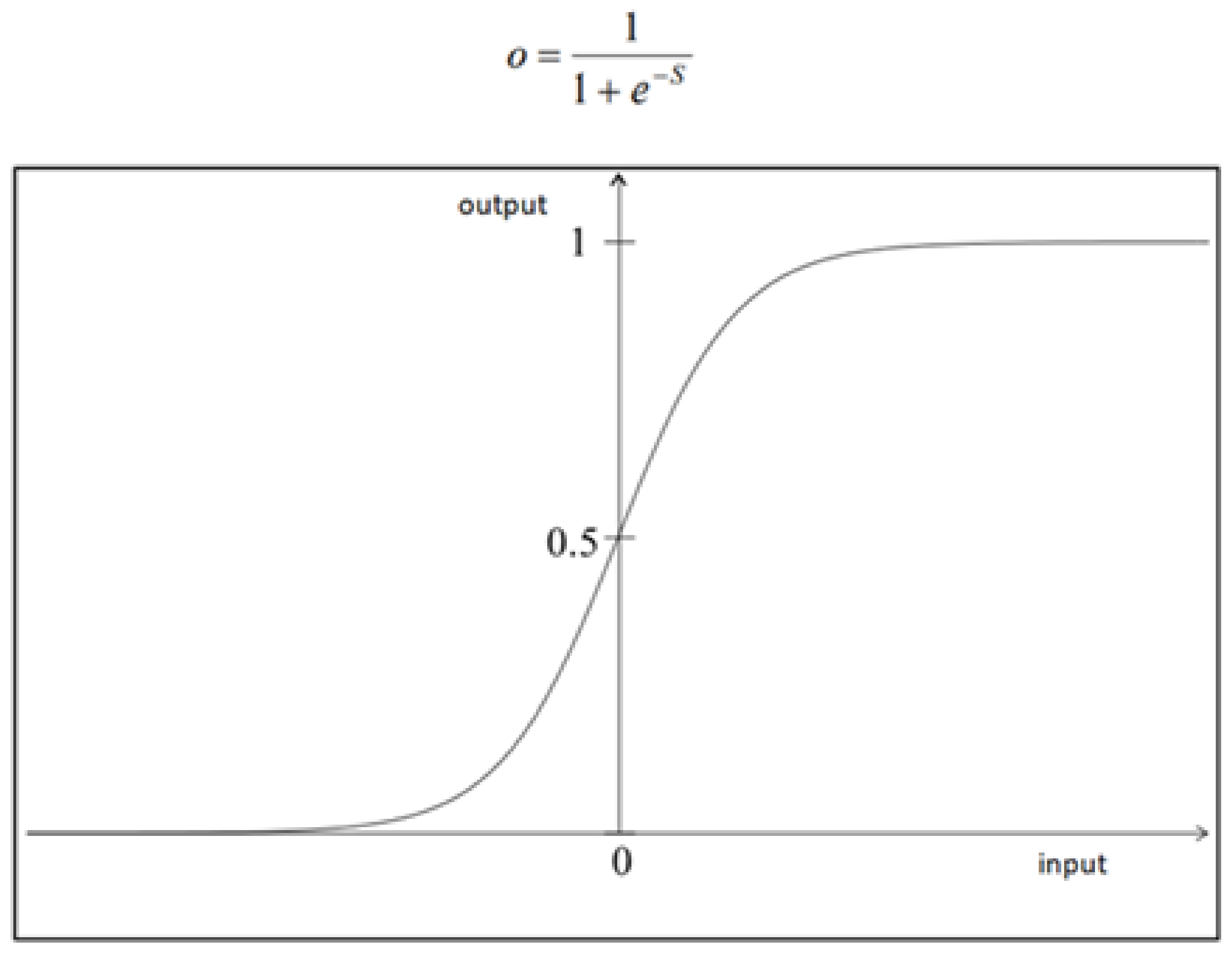
Figure 1, neurons of different levels are connected by a line. At this point there is no general rule, i.e., how many and which neurons are connected to whom. In one case each neuron could be connected to all the other neurons, of all levels (maximum number of connections). Alternatively, a network with multiple levels of each neuron could be connected to just one other neuron (the minimum number of connections it can have). In intermediate cases there are usually some connections between neurons. Obviously, the number of connections, especially for full wiring is very large. If we have N neurons, then the number of connections in complete wiring is N (N − 1)/2. The training process is similar to the sensor, but has some essential differences. The signal comes to each input level neuron (the first level). Multiply by the corresponding weight w of each conclusion. In each neuron the arriving products are added and the S is calculated, as in the sensor model. However, there is an essential difference here. While in the sensor the sum is compared to θ, here something different happens. There is a representation (activation) function, which is typical of the network, and which is used each time to calculate what the output value will be. Suppose the output value is o. A commonly used function is shown on
Figure 2.
The value of o is always 0 <
o < 1, for any value of input
S. This is important, because that way we are sure that there will be no cases where the output takes large values or tends to infinity. This curve is called sigmoid because of its shape. It is an ideal function, because it behaves well for all price sizes. For small values of
S the slope is large, and so the output is not almost 0. Accordingly, for large values of
S the slope is normal, so that the network cannot be saturated. Another property of this function is that its derivative also behaves well, which is necessary in the training process, below. We easily show the following equation:
Another name for the function o is compressed function, because it compresses any value of S in the interval between 0 and 1. We also observe that this function is non-linear, a necessary condition for the network to be able to generate signal representation. This overall process is a cycle, i.e., a passage, entry-exit-entry, and summarizing includes the following steps:
We get a pattern from the many. We enter it at the entry level.
We calculate the output.
We promote it in the same way at all levels up to the final output level.
We calculate the error.
We change weights, returning from exit to entry, one by one, and level-by-level.
We move on to the next template.
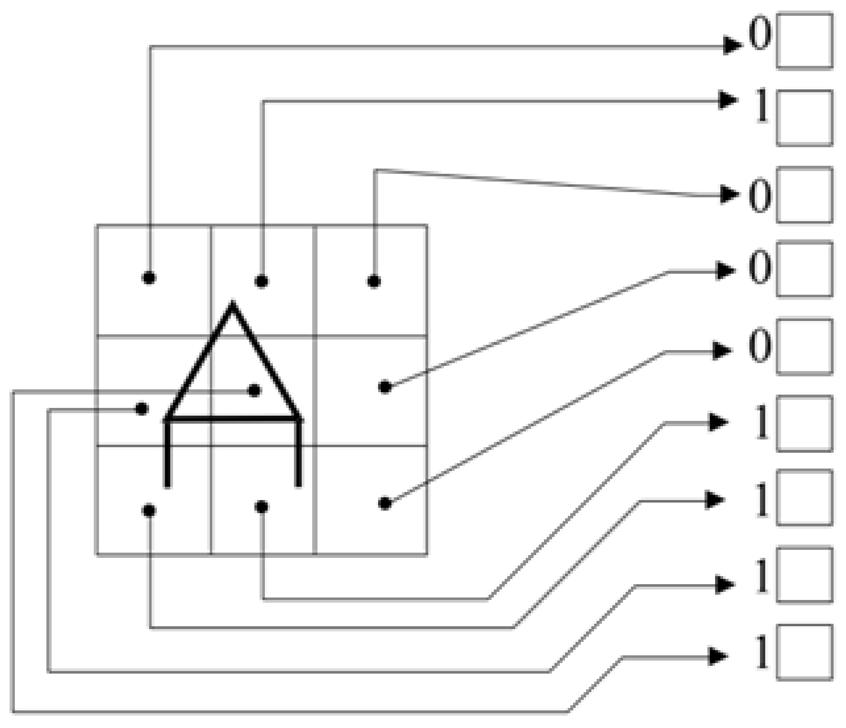
At the end of a cycle, repeat the process for as many cycles as needed, until the error is small enough. The tolerance for the error is given in advance, and standard values are a few % units, e.g., 2 or 5%. An example of a target pattern pair is given in
Figure 3, where the letter A is plotted on a grid. If any line passes through a square, then the input to the corresponding neuron is 1. Otherwise, the input is 0. The output can be a number representing A, or another set of 0 and 1. For the whole alphabet we need 24 network training pairs, one pair for each letter. The error reversal training method uses the same general principles as the Delta rule. The system first takes the inputs of the first standard and with the procedure described previously produces the output. It compares the output value with the target value. If there is no difference between the two nothing happens and we move on to the next pattern. If there is a difference then we change the values in such a way that this difference is reduced.
5. The Training Method for Linear Neurons
In this methodology the goal is for each neuron and for each pattern to minimize the square of the difference between the received neuron output and the desired value (target). This means that the derivative of the error with respect to each weight w is proportional to the change in the value of the weight, as given by the Delta rule, with a negative ratio constant. This is proportional to the steepest descent process on the surface in the weight range where the height is equal to the error value. The above applies to linear units of neurons.
where
Ep is the error (input-output difference) in template
p,
tpj and
opj is the target and output of neuron
j for template
p. The total error
E is:
For linear units we apply the Delta rule, and we actually have a gradient descent in
E. We show that:
When there are no hidden units then the derivative is calculated immediately. We use the chain rule and write the derivative as a product of two other derivatives: one derivative of the error with respect to the output of the neuron on one derivative of the output with respect to weight.
The first derivative tells us how the error in the output of the
j neuron changes, while the second part tells us how much the change in
wji changes this output. This is how we directly calculate the derivatives. The contribution of neuron
j to the error is proportional to
δpj, since we have linear units.
from which we conclude that:
Substituting Equation (5) we see that:
exactly as we want. Combining the latter equation with the observation that:
leads us to the conclusion that the change in
wji after a complete cycle, where we present all the patterns, is proportional to this derivative, and therefore the Delta rule applies a sloping descent to
E. Normally
w should not change during the cycle where we present the various patterns, one by one, but only at the end of the cycle. However, if the training rate is low, no big mistake is made and the Delta rule works properly. Finally, we will find the values of
w that minimize the error function.
6. The Training Method for Non-Linear Neurons
We have shown that the Delta rule results in a sloping descent squared of the error sum for linear actuation functions. In case we do not have hidden levels, the error surface is like a bowl with only one minimum, and so the sloping descent will always find the best values for the weights w. In the case of hidden levels, it is not obvious how the derivatives are calculated and the error area is not concave upwards, so there is a chance of being at a local minimum. We will show below that there is an effective way to calculate derivatives, and that the problem of local minimums usually does not affect network training. We use here networks with multi-level structures in which the signal is always propagated in the same direction, from the input level to the output level (feedforward). The signal comes at the input level, at the lowest level, is processed by the network, and forwarded to the hidden levels. The hidden levels process it and push it to the output level. The processing is always done level by level, on each neuron separately. Activation is calculated in each neuron, using the non-linear function, taking as input the output of the previous level, and giving as output to the above level the calculated value. For such a nonlinear function the output is:
where
opi is the input signal of neuron
i. Therefore,
where
f is a differentiable and increasing function. Linear functions are not enough here, because their derivative is infinite at the threshold, and zero at other values. We suppose that:
where
E is the error function (sum of squares). Here we put this derivative as a product of two derivatives: one that gives the change in error with respect to the change in the input value, and one that gives the change in the input value with respect to the change in weight. So:
We define that:
where
δpj = (
opj −
tpj), as well as
opj =
Spj when the neurons are linear. So we have:
This indicates that to apply the sloping c to
E we must make the changes to
w as follows:
just like in the usual Delta rule. Now we need to calculate the correct
δpj for each neuron in the network. Here, we put this derivative as a product of two derivatives: one that gives the error change as a function of the output, and one that gives the output change as a function of the input change. So, we have:
but we have:
which is the derivative of the activation function for neuron
j, calculated at the input signal
Spj to this neuron. Now we compute the first derivative in the equation
δpj. Here you need attention. We calculate this factor differently if the neuron is at the output level or internally. In case it is at the output level then:
which is the same result as with the usual Delta rule. By substituting the two factors we get:
for neurons that are at the output level. For neurons that are internal there is the problem that we have no
tpj, i.e., we do not have target values. In this case we have:
Substituting similarly we get:
These equations give the way in which all d, for all neurons in the network, are calculated, and which are used to calculate the change in
w across the network. This procedure is considered to be a general delta rule. In summary, the above procedure can be summarized in three equations. First, we apply the general Delta rule in the same way as the general rule. The
w in each level changes by a quantity that is proportional to the error signal
δ, and also proportional to the output
o. That is,
The other two equations give the error signal. The process of calculating this signal is a cyclic process that starts at the output level. For a neuron at the output level the error is:
where
f’j (
Spj) is the derivative of the activation function. For neurons in hidden levels is given by:
These three equations form a circle. The system repeats as many cycles as it takes to train.
7. X-OR Problem Simulation
We will now solve the well-known X-OR problem with a grid containing a hidden layer, as described above and shown in
Figure 4. The network structure includes two neurons at the input level, one neuron at the hidden level and one at the output level.
The connections are as in the figure. It is necessary that the entrances go both to the hidden level and to the exit directly. This problem is of didactic importance, as its solution includes all the details of the backward propagation technique, and for this reason we will outline its solution by a simulation method, following one by one the steps and equations. We use an equation to calculate the outputs of each neuron, the sigmoid function, as:
where
θj is the predisposition parameter (or predisposition) and which in a way plays the role of the threshold. The values of predisposition,
θj, will be taught in the network, as well as the values of the other weights
w. Indicates the weight
w of a unit (neuron) that is always active. The derivative
opj (1 −
opj) has a maximum for
opj = 0.5, and approaches its minimum when
opj approaches 0 or 1, such that 0 ≤
Opj ≤ 1. The change in a
w is proportional to its derivative, and so the ws will change more if we have a mean value, i.e., neither active nor inactive. This feature gives the system solution stability. It should also be noted that when checking for output values 0 or 1, it is impossible to get exactly these values unless we have
w that tends to infinity. Usually, it is enough when we get 0.1 and 0.9, even if we mention 0 and 1. This accuracy is reached. The equation of the change of
w has a constant, the
n, which represents the training rate of the network. The larger the
n, the greater the changes in
w, and the faster the network trains. However, if it does not become very large, then this leads to oscillations, and so we are forced to not be able to increase it much. One way to increase the pace of training and avoid fluctuations is to include another term that indicates the momentum of the system. Thus, the equation becomes:
where
n denotes the cycle, or the rate of training, and
α is the constant that takes into account the previous changes of
w when calculating the new change. This is a form of system momentum that essentially filters out high-frequency changes to the error surface. Usually, we get a value of α which is
α = 0.9. We first assume that the weights
w1 =
w2 =
w3 =
w5 = 1. The value
w4 = −2 from the hidden neuron to the output neuron renders the output neuron inactive when both inputs are active at the same time. The numbers inside the neurons are the values of
i. At the hidden level
θ = 1.5 because then this neuron will only fire when both neurons of the first level are active. The value
θ = 0.5 on the output neuron makes this neuron active only when it receives a positive signal greater than 0.5. On the output neuron side, the hidden level neuron appears as another input unit. It sees it as if there were three input values. Of course, these prices are purely indicative, and not necessary for the solution of the problem. Applying the simulation method now, we solve the X-OR problem, so that the network can successfully find the patterns and the number of cycles needed to do this, given in
Table 1. In the solution given below we start with random values of
w that range in the range −0.3 <
x < 0.3.
The values in table are averages of ten embodiments, with different values of w each time. We observe that the standard deviation has a large value, which shows that the solution is directly dependent on the initial w.
Summarizing the solution of this problem, we give the flow chart, as well as the equations in
Figure 5 below.
8. Machine Learning Human Activities in Smart Home
A smart home now through Deep learning provides a high level of services, both in terms of safety and health care, with the ability to record and recognize face and human activity using a depth camera. Until now, efforts are made to optimize such systems in order to raise the quality of daily life and especially of the elderly with daily and continuous recording of human activity. Inside the house, the system records on a continuous daily basis, and acquires knowledge and experience in recognizing behaviors and events; this is valuable knowledge that increases its performance and consequently increases the level of quality of services provided. Such a system supports real-time life recording, through human activity recognition, based on depth imaging. A depth imaging device is used to capture depth silhouettes when recording human activities. Thus, information is extracted from the human silhouettes, from the parts of the body that are used to identify activity, training the machine in the human routine in everyday life.
The machine learns to recognize human activities. First, it is trained through a depth camera in the recognition and recording of human movement, then in recognizing the existence of human action, in recognizing the human silhouette, in extracting its characteristics and in recognizing and classifying its activities. This process eventually leads the machine to have a record of human life with human activities, something that makes it even in real time, through a camera, capable of being able to recognize daily human activities.
A modern approach has been evaluated against the life recording system using conventional master components (PCs) and it has been shown that the use of Radon transformations in depth silhouette features has achieved a higher recognition rate. Real-time experimentation has shown that the result for the feasibility and functionality of the applied system is that the system could be used to create lifetime logs of human activities in smart homes. This makes living at home safe and easy in a smart living space, with sensor technologies (i.e., sensors and video recording) integrated into a system that stores the activities of the user’s daily life. The system includes a life diary, which is a virtual diary containing information on a person’s daily activities, performed by a range of sensors and videos, which can be integrated into everyday devices with different applications, for example to provide health care services for the elderly and security monitoring in a smart home. A life recording system is referred to as a mechanism, which creates life recording files, which contain the daily activities of man indoors (e.g., in a smart home, smart offices, etc.) through the recognition of human activity (recognition of human activity/HAR). Usually various sensors, such as motion sensors, video sensors, or RFID (Radio-frequency identification), are used in HAR. Such a life recording system can provide continuous monitoring and recording of the daily activities of the inhabitants. Therefore, the life recording system HAR is one of the most basic processes.
Based on these automatically recorded HAR life systems, such a system can examine the life patterns of human activities, in order to improve the quality of life, by analyzing daily habits or planned/regular actions (human routine) and manifestations of human life, such as sleeping, medication, office schedules, or taking a meal, depending on the person’s lifestyle. Life recording systems use electronic devices, such as portable motion sensors and video sensors (i.e., video cameras). In the motion sensors where the system is based, they are connected to the user. The motion signals are then recorded and analyzed to create the characteristics of the various human activities. Through these features, activity recognition is performed to create a routine of human life.
The technologies of portable motion sensors have been extensively presented for the recognition of daily activities in the recording of life in 2014 at the 11th IEEE International Conference on Advanced Video and Signal Surveillance (AVSS), with results of recognition of conventional and proposed approaches to life recording. Comparing the life record system to conventional approaches using depth silhouettes, we have an improved recognition rate for almost all smart home activities. Based on experimental results, the proposed life recording systems, using Radon recognition, achieved improved recognition by up to 89.33% compared to conventional systems, where PC functions achieved 71.25% and 78.58% using depth silhouettes. This system is directly applicable in many areas of daily life by consumers, such as smart homes for its residents, especially the elderly, in order to monitor their health, with a monitoring system, as it creates a diary of activities of elderly people with the aim of improving their quality of life [
18].
9. Face Recognition System in Smart Home
A facial recognition system [
19,
20,
21,
22,
23,
24] deals with the automatic identification or identification of a person from a digital image or video. One way to identify is to compare selected facial features from the image with features from other people in a real-time database.
There is a face recognition system, almost real-time in everyday and affordable consumer applications. The system responds differently and provides personalized services for each user individually. Each home environment is separate and unique, as is the system input data and the end services to the user. Now a face recognition system is a great and powerful helper in the hands of the consumer based on the level of quality of life. In a smart home the system operates over a home network that monitors and records the home environment with low-cost equipment. To enable distributed computations, a face recognition treatment line is used, which operates in stages: (1) gradual “pruning” for face detection, (2) thick to fine face extraction, for face smoothing, and (3) face recognition with sequential discrimination analysis. The system has been implemented in various environments, such as an experimental home network and has achieved a recognition rate of over 95% and a processing speed of 3 to 4 frames/second.
This system is a fast built-in face recognition system, for smart home applications. In contrast to the very limited recognition of a person in real life, by systems that operate under controlled environments, this system focuses on real life, in unrestricted and completely controlled environments, with a very satisfactory recognition rate. In addition, processing efficiency and low cost are the main advantages of this system, as it covers all the basic functions of face treatment, i.e., face detection, face feature extraction for face normalization, and finally face recognition.
During each processing step, gradual improvements are used for improved robustness and efficiency. The system achieves a recognition rate of over 95% and a processing speed of 3–4 frames/second. The face recognition system operates in an environment with no operating restrictions and offers high processing efficiency using low-cost material. This is especially attractive for simple, everyday consumer applications, where easy-to-use and user-friendly interfaces and low cost are of the greatest interest.
It is widely accepted that the process of face recognition requires very powerful processors with great computing power. Therefore, it must be done in such a way as to achieve the best result because this will improve the performance of the system as a whole. To achieve this, it must be done in a distributed way, such as face detection at the entrance of the house, processing to extract features, and face recognition to be performed on a multimedia server in the house. The current HomeFace system is able to handle the front of the face, with off-plane rotation within ±20 degrees (future research is required to deal with large head rotations) [
25].
10. Methods of Facial Recognition
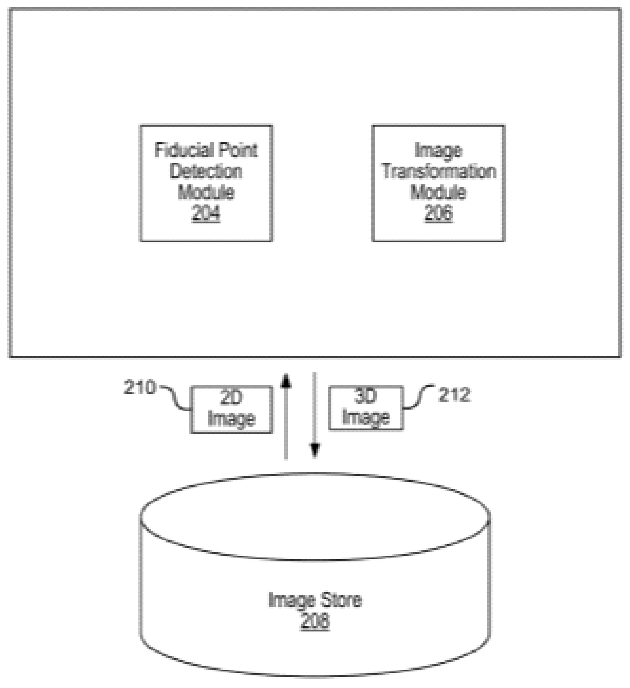
Using deep machine learning with neural networks a machine is able to recognize, classify, and align facial images; using a 2D image the machine can output an aligned 3D image. In this process, with the classification and alignment of the 2D face image, the face recognition is done. The unique characteristics of a person are identified as a set of vector values which will give the unique identity of the person depicted.
The algorithm recognizes the identity of a person using an image or video, without human intervention. Face recognition in everyday images, taken under real-world conditions, is a pioneering and revolutionary algorithmic concept. However, this ability of the machine to recognize faces, although it tries to imitate the human brain and eye, still far from it, presents a large percentage of errors. The system can still be improved, an effort that has been largely made in recent decades, when recognizing two-dimensional images of faces, taken in completely controlled and limited environments. The methodologies include sketching—control and intelligent biometric identification. However, the capabilities of the system are dramatically limited when the conditions are in a real environment, where there is limited lighting, facial expressions, and aging. Generally, when the conditions are uncontrolled and unplanned in the system specifications the performance drops significantly.
Various integrations of the face recognition application may include systems, methods, non-transient computers and readable media configured for face image alignment, face image sorting and image verification using a second identity to determine if both identities are identical and belong to the same person, through a neural network.
In some versions of the system, through the aligned 2D image an 3D is extracted. The face recognition is performed in the 2D image. This happens through neural networks and is classified using the aligned 3D image. The identification performed in the 2D image includes a set of features. In a real system application, a set of 2D key points is located in the image. The 2D face image can be used to produce a 3D shape to then create the 3D aligned face image. In such an application, a set of “anchor” points can be placed, on which the system for forming the 3D shape will be based. In a deep machine learning application in a 2D image its key points must be identified as a set of triangles/anchors. The key points of a two-dimensional image that make up the anchors can be displayed either on the back of the 3D image or on the front. These sets are the anchor points from which the aligned 3D image is extracted by applying the “Affine” transform to each triangle.
During the conversion application, a part of the face of an image can be identified by detecting a second set of key points in the image. This set can lead to the formation of the whole 2D image. In fact, a set of anchors is determined from the 2D image from where the image is formed. the DNN consists of a layer of maximum concentration and a convergent layer, which extracts the three-dimensional aligned points of the face in each of its functions when connected to each of its adjacent layers.
Each set of connected layers is configured to export the correlations between the 3D aligned points of the face as a feature face vector. These vectors are then used by DNN to sort the 3D image. Each feature of the 3D image is identified by the feature vectors and is normalized to a predefined range. With defined filters, each pixel is assigned a three-dimensional aligned point. The machine learns to define the filters itself based on the set of data/vectors it has at a time.
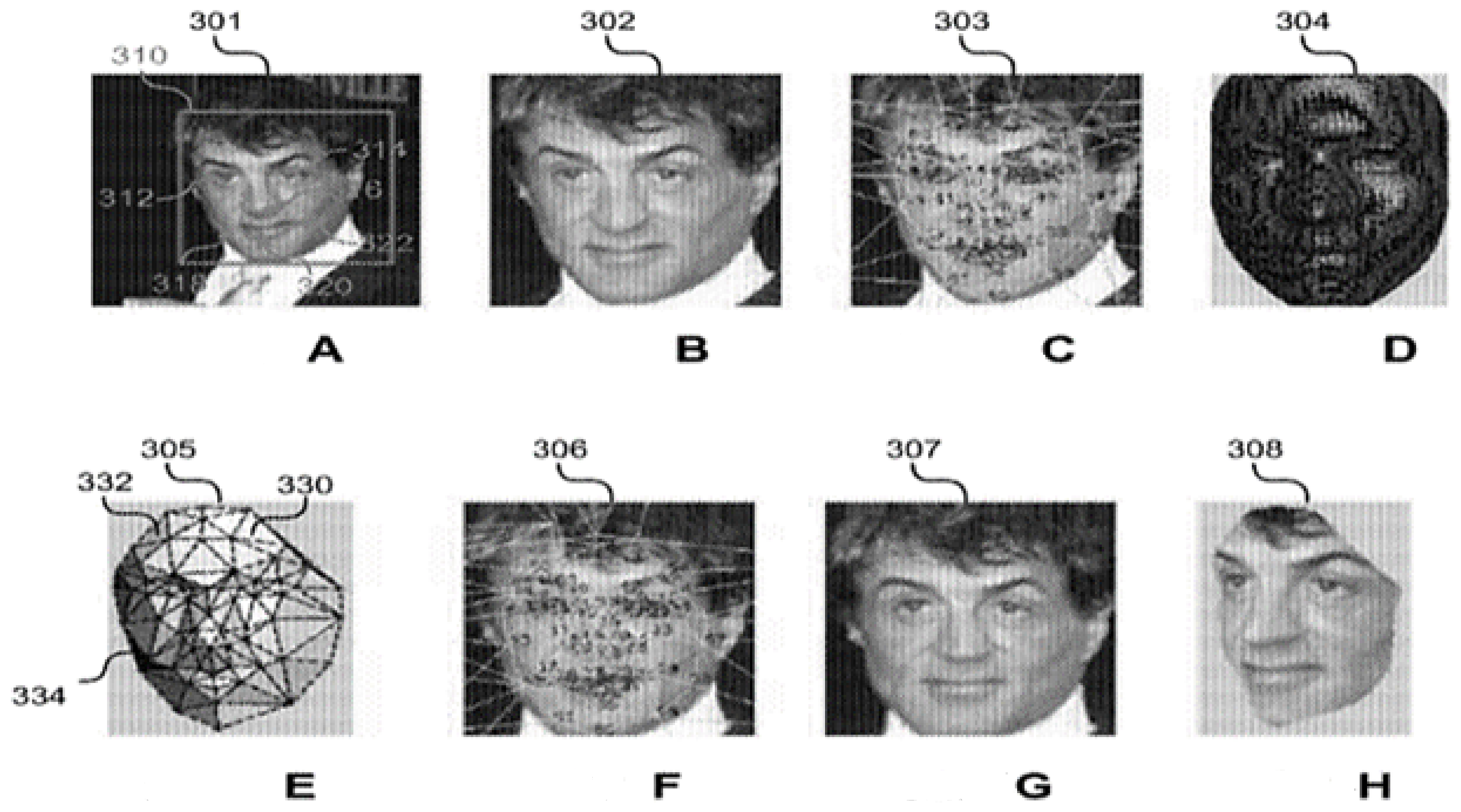
A 2D face image can be identified through a database of images. Face images are stored in a face database, where there are sets of images and each set corresponds to a face. A set of features is the face ID. Each face ID derived from a 2D image is sorted based on a unique value assigned to it when executing an DNN between its adjacent layers. Based on this classification, the faces are separated, after a comparison is made between the identifiers and the identity of the person depicted in the image is given in
Figure 6 and
Figure 7.
11. Face Recognition Application Using Fog and Cloud Computing Technologies
Face recognition is now performed with a suitable application and from mobile smart phones. The owner of the mobile has only to take a photo of his face or someone else and the application sends it to a remote server using fog or cloud platform. There is stored a local database with pictures of faces from which the identity of the depicted person will be retrieved. This application is very popular nowadays. In an experiment performed: “the application running on the smartphone takes 384 × 286 pixel photos, the face photo database on the remote server consists of 1521 photos, each of which is also 384 × 286 pixels.” The same tasks are performed in both fog and the Amazon Cloud EC2.
In [
26] the authors estimate the Face recognition time and Response Time for Fog and Cloud as following: for Fog the Face recognition t is 2.479 ms and the Response Time is 168.769 and for the Cloud is 2.492 ms and 899.970 ms respectively. The ‘Response Time’ in [
26] is the time period from when the smartphone starts uploading the photo of the face and when the smartphone receives the result from the remote server. Providing similar capabilities VM (virtual machine), in fog and cloud, we observe that similar time was consumed in the computational work (about 2.5 ms in each case). From
Table 2 and
Table 3, we understand that the difference in latency between fog and cloud is small (less than 10 ms). Therefore, network bandwidth contributes more to the large difference in response time (731.201 ms). Assuming that the smartphone can upload a face photo in negligible time in the fog, then the smartphone can upload about 167 KB of data in the cloud to that of 731.201 ms, which is comparable to the average size of uploaded face photos (about 110 KB)” [
26].
12. Human Silhouette/Figure Recognition System
Human identification can be done using video stream output data classification methods. In addition to the Deep learning method, both SVM (Support Vector Machine), decision tree and Bayes are used to determine the exact human body position. However, the machine, through the Deep learning method, is able to recognize with absolute accuracy up to 100% the positions of the human body, as opposed to other methods that reach 93.72%. The human positions that the system recognizes are as follows: standing, sitting, and lying down. First, 20 human joint position vectors are entered into the system, then the machine recognizes and classifies the three human positions. The procedure is performed using a Kinect camera at a distance of two to three meters from the human body.
In the future, this application will be used as a basis for the analysis of time series of sequences of positions of the human body, for motion and fall detection, in an intelligent home system [
27].
13. Conclusions
In this study we presented the methods that have been developed to create smart homes, analyzed methods such as Back Propagation for neural networks for the purpose of machine learning, which mainly focus on face and silhouette recognition, without ignoring the huge contribution of machine learning and in other sciences such as medicine.
Security systems focus on face recognition to improve security in and around the home, in order to improve access, make them more familiar to users, and create a seamless experience in smart homes or buildings.
Today companies such as Netatmo, Netgear, Honeywell, and Ooma have gone so far as to incorporate face recognition technologies into their home security systems that help identify people approaching the home and detect potential intruders. When everyone is absent from it.
Honeywell has partnered with Amazon Alexa to design and market a unique home security system that will offer a perfect solution for those who want to build a smarter home in many ways, not just security.
Today, Google Nest Cam IQ monitors your property 24/7 and can locate people from a distance of 50 m. The system can identify familiar faces and you can predetermine actions for these visitors, such as opening a gate or a front door.
While face recognition undoubtedly changes the world we live in, the world is also changing the way face recognition is developed around the world in terms of security, which is critical nowadays, as well as in all others areas of our lives [
28,
29,
30,
31,
32,
33,
34,
35,
36,
37,
38,
39,
40,
41,
42,
43,
44,
45].


 and
and 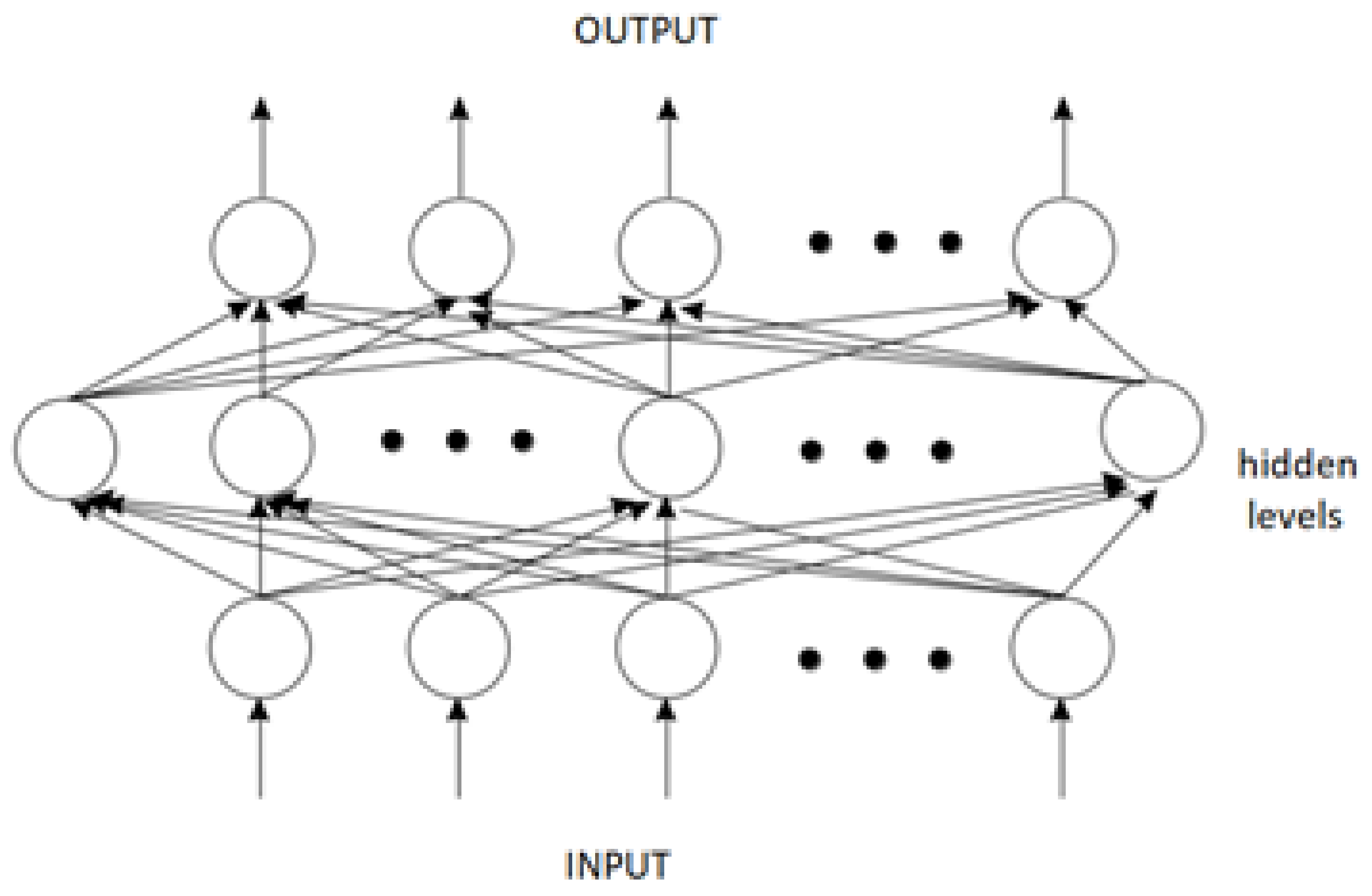


